HAL Id: hal-00001129
https://hal.archives-ouvertes.fr/hal-00001129v3
Preprint submitted on 13 Feb 2004
HAL is a multi-disciplinary open access
archive for the deposit and dissemination of
sci-entific research documents, whether they are
pub-lished or not. The documents may come from
teaching and research institutions in France or
abroad, or from public or private research centers.
L’archive ouverte pluridisciplinaire HAL, est
destinée au dépôt et à la diffusion de documents
scientifiques de niveau recherche, publiés ou non,
émanant des établissements d’enseignement et de
recherche français ou étrangers, des laboratoires
publics ou privés.
for Elementary Cellular Automata
Nazim Fatès, Michel Morvan
To cite this version:
Nazim Fatès, Michel Morvan. An Experimental Study of Robustness to Asynchronism for Elementary
Cellular Automata. 2004. �hal-00001129v3�
ccsd-00001129 (version 3) : 13 Feb 2004
Asynchronism for
Elementary Cellular Automata
Nazim A. Fat`es∗Laboratoire de l’Informatique du Parall´elisme, ENS Lyon, 46, all´ee d’Italie 69 364 Lyon Cedex 07 - France
Michel Morvan†
Laboratoire de l’Informatique du Parall´elisme, ENS Lyon, 46, all´ee d’Italie 69 364 Lyon Cedex 07 - France
Cellular Automata (CA) are a class of discrete dynamical systems that have been widely used to model complex systems in which the dynam-ics is specified at local cell-scale. Classically, CA are run on a regular lattice and with perfect synchronicity. However, these two assump-tions have little chance to truthfully represent what happens at the microscopic scale for physical, biological or social systems. One may thus wonder whether CA do keep their behavior when submitted to small perturbations of synchronicity.
This work focuses on the study of one-dimensional (1D) asynchronous CA with two states and nearest-neighbors. We define what we mean by “the behavior of CA is robust to asynchronism” using a statistical approach with macroscopic parameters and we present an experimen-tal protocol aimed at finding which are the robust 1D elementary CA. To conclude, we examine how the results exposed can be used as a guideline for the research of suitable models according to robustness criteria.
1. Introduction
The aim of this article is to study the robustness to asynchronism for cellular automata. In other words, we propose to examine some qualitative and quantitative aspects of the change of behavior that are induced when the cells are no longer updating their state systematically at each time step.
The first study of the effect of asynchronism was carried out in 1984 by Ingerson and Buvel in [19] :
“ (...) Cellular automata exhibit such remarkable self-organization ∗Electronic mail address: Nazim.Fates@ens-lyon.fr
†Electronic mail address: Michel.Morvan@ens-lyon.fr
that it is certainly tempting to consider the possibility that they may be a valid model for real-world systems, such as the growth of biological organisms, crystals, snowflakes, etc. However, one commonly made assumption about these systems is that the cell iterate synchronously. We wanted to estimate how much of the interesting behavior of cellular automata comes from syn-chronous modeling and how much is intrinsic to the iteration process.”
The authors carried out experiments on the space of “elementary cel-lular automata” rules (see 2.2) and showed that varying the iteration process produced significant change in the evolution of some cellu-lar automata whereas some other cellucellu-lar automata were not affected by the modifications. The study was however purely qualitative and no algorithmic method was proposed to systematically estimate these changes.
In 1993, Huberman and Glance criticized the use of CA as a mod-eling tool that could be suitable for describing real-world phenomena [11]. The model they studied is a spatially-extended version of the prisoner’s dilemma “with no memories among players and no strategi-cal elaboration” introduced by Nowak and May in [14]. They argued that the model was not realistic because it used the assumption that the actors all updated their strategy synchronously. Their experiments showed that when the perfect synchrony assumption was dropped, sig-nificant changes of behavior were observed. At the same time, similar ideas were developed by Stark in the field of biology[18].
In 1994, Bersini and Detours studied an asynchronous version of the Game of Life [2]. They observed that the introduction of asynchrony led to modifying the dynamics from a behavior with long transients to a behavior with fixed points. The authors explained this property by identifying some asynchronous CA with Hopfield neural network and by proposing a description of the asynchronous behavior in terms of Lyapunov energy functions. This raised the question to know whether the stabilization effects was to be observed for any model or was specific to the models chosen by the authors. This article partially answers this question by exhibiting counter-examples for which the increase of asynchronism leads to less stability (see Section 3.5.3).
The first quantitative study of the influence of the way transitions were made in CA were carried out by Sch¨onfisch and de Roos [17]. The authors use explicit functions for updating the cells and show that the evolution of a cellular automaton might strongly depend on the corre-lation between the spatial arrangement of cells and the order of their update. For example, if the cells are arranged in a line, one could con-sider the possibility of updating the cells one-by-one from left to right. The correlation between the updating method order and the spatial position of the cells is analytically estimated and it appears that for
some type of updating methods, the evolution of the cellular automa-ton becomes strongly dependent on the lattice size. The important result is that among the different update methods studied, the only method which did not introduce any spurious correlations consisted in choosing the cells of the lattice randomly with an equal probability for each cell. In the study we here present, we only consider this partic-ular type of asynchronism and rather concentrate on the study of the phenomenological changes observed.
The purpose of this work is to propose a first algorithmic approach to answer to the question “To which extent is the behavior of cellular automaton dependent on the synchrony of the transitions?”. In other words, we want to know if the application of a small change in the way the transitions are performed leads to brutal changes of the “behav-ior”. Note that this differs from studying the effect of perturbing the configuration themselves, for example introducing noise in the system. In Section 2, we give formal definitions of the CA concepts and we describe the algorithm we use to quantify CA robustness. In Section 3, we analyze the results by sorting the models according to the ro-bustness quantification given by our protocol. In the last section, we discuss the results and analyze how the study of robustness could be related to the activity of modeling complex systems with CA.
2. Definitions and experimental protocol
In this section, we formally define the notion of asynchronous cellular automaton. We then describe the experimental protocol used to quan-tify the robustness of a model using the notion of “sampling surface” and the notion of “robustness indicator”. Finally, we analyze some intrinsic limits of our protocol.
2.1 Asynchronous Cellular Automata
An Asynchronous Cellular Automaton (ACA) is a 5-tuple (L, Q, G, f, ∆) defined as follows :
A cell is a variable that takes its values in Q, the set of possible states. The set of all cells is called the lattice, it is denoted by L and we have L ⊆ Zd, where d is the dimension of the lattice.
The neighborhood of a cell N (c) is a function which associates to a cell c an ordered set of cells. The cardinality of N (c) is constant and is equal to N .
f : QN → Q is the local transition rule which defines how a cell updates its state according to the states of the cells located in its neighborhood.
∆ : N → P(L) is the updating method [17], which defines for each time t, the set of cells to which the transition rule is applied. In a modeling approach, ∆ might be seen as defining the set of non-defective cells at time t, with the convention that a defective cell will keep its state constant whereas a non-defective cell will update its state according to the local rule.
The updating method ∆ is said to be synchronous if ∀t, ∆(t) = L, otherwise it is asynchronous. In this context, it appears that “classi-cal” Cellular Automata form a particular sub-class of ACA, for which the update rule is synchronous. We restrict here our study of updat-ing methods to the sub-class of step-driven methods [17], in which the expression of time does not appear explicitly in the definition of ∆. Among all the possible step-driven methods, we choose to use asyn-chronous stochastic dynamics, denoted by ∆α, defined by considering
for each time t every cell of L and assigning a probability α that this cell is in ∆(t). The parameter α ∈]0, 1] is called the synchrony rate. This updating method has the advantage of satisfying a “fair sampling condition” which specifies that each cell should be updated an infinite number of times without any bias1 :
∀c ∈ L, lim T →∞ card {t ≤ T, c ∈ ∆(t)} T = α card L .
An assignment of a state to each cell of L is called a configuration. It is denoted by x = (x(c))c∈L, with x ∈ QL. ∆ being fixed, the global
transition functionis a function F∆ : QL× N → QL which associates
to each configuration x = (x(c))c∈Land to each time t, a configuration
y = (y(c))c∈L such that :
y(c) = f [N (c)] if c ∈ ∆(t) y(c) = x(c) otherwise.
A global transition function is a particular kind of discrete dy-namical system acting on configurations. We thus can associate to each configuration x its orbit, the series of configurations (γα(x, t))t∈N
obtained by the iteration of F∆α on x using the recursive definition
γα(x, t+1) = F∆(γα(x, t), t). However, unlike dynamical systems which
do not depend on an update function, when the updating method is not synchronous (i.e, when α < 1), the orbit of γα(x, 1) is not
necessar-ily the shifted orbit of x = γα(x, 0). We will say that a configuration
xf is a fixed point if ∀∆, ∀t, F∆(x, t) = x. Finite parts of the orbits
1
In [1], the definition of the “fair sampling condition” only imposes that each cell should be updated an infinite number of times. In our context, we have chosen to add the property that each cell should also be chosen with an equal probability to any other cell.
can be represented in space-time diagrams, where configurations are represented horizontally and where time is represented vertically (see Figure 1).
Figure 1.Example of space-time diagram of ECA 128 (see 2.2 for coding). Configurations are displayed horizontally and time goes from bottom to top.
In the sequel, we will be interested in some configurations in which the transition of information is blocked. We say that a word w ∈ Q∗is
a wall if it verifies : ∀(u, v) ∈ Q × Q, F|w[uwv] = w, where F|w denotes
the restriction of F on the cells that compose w. A wall is a “strong” type of blocking word (i.e., a word that splits a configuration into two parts by preventing any information to cross it [8]). We will call a q-domaina set of adjacent cells that are all in state q.
2.2 One dimensional Elementary Cellular Automata
In this paper, we restrict our study to the one-dimensional case, taking d = 1. We call elementary cellular automata the class of 1D-ACA defined by Q = {0, 1} and ∀c ∈ Z, N(c) = {c − 1, c, c + 1}. As the study is experimental, we only consider lattices of finite size, using periodic boundary conditions : 1D lattices are rings and indices of L are taken in Z/nZ, with n size of the ring.
Following [20] we associate to each ECA f its code :
W (f ) = f (0, 0, 0) · 20+ f (0, 0, 1) · 21+ · · · + f(1, 1, 0) · 26+ f (1, 1, 1) · 27.
we will equally use the more general word ’model’ to qualify a rule. The symmetry operations obtained by the left/right exchanging and 0/1 complementation allow to associate to each rule R, a reflected rule Rp, a conjugate rule Rc, and a reflexive-conjugate rule Rcp. The association of R to (R, Rc, Rp, Rcp) allows the partition of the ECA space into 88 equivalence classes and we will call minimal representativethe rule that has the smallest index in a class. In the sequel, we will work in this quotiented space and we will only consider minimal representative rules.
2.3 Experimental protocol for robustness estimation
The purpose of this section is to introduce formal notations that allow to specify the protocol we use to obtain the experimental data. We then introduce the concept of ’sampling surface’ to qualitatively estimate a model’s robustness to asynchronism and we propose to quantify this robustness using two parameters. Finally, we analyze the limits of our protocol.
2.3.1 Definition of the protocol
The macroscopic measures we use to estimate the change of behavior of an ECA are based on the statistical analysis of the density variations. The density of a configuration is a real number defined by ρ : QL →
[0, 1] such that ρ(x) = #1(x)
|x| where #1(x) denotes the number of 1’s
in x and |x| is the size of the configuration x. In a previous work [10], we showed that the density and more precisely the evolution of the density can be considered as a pertinent parameter for describing in a first approximation the global behavior of an ECA. For example, it can be used as a means of discriminating the chaotic-looking ECA from the regular-looking ones.
The density is used here to identify the models that are non-robust to the introduction of asynchronism. In order to have an “observation function” µ that will quantify changes in behavior, we use an experi-mental protocol that depends on five parameters :
The size of the grid n.
The density of the initial condition dini. The initial condition x(dini) is constructed using a Bernoulli process : for every cell of x, this cell has a probability dinito have state 1 and a probability 1 − dinito have state 0. The distribution of the density of x is binomial, which implies that d(x) is close to dini for large |x| with high probability but note that it is not often strictly equal to dini.
The synchrony rate of the update method α.
The sampling time Tsampling during which the orbits are analyzed.
In order to obtain µ experimentally, we take the initial condition x(dini) and let the ACA defined with synchrony rate α evolve during
Ttransient steps. We then store the value of the density during Tsampling
steps and average this value to obtain µexp(dini, α) :
µexp(dini, α) = 1
Tsampling
t=TtransientX+Tsampling
t=Ttransient+1
d(γα(x(dini), t)) .
Algorithm 1 Construction of a sampling surface
for dval = dmin to dmaxstep dstp do
xini(dval) ← random initial condition of density (dval) end for
for α = αmin to αmaxstep αstp do for dini= dmin to dmaxstep dstp do
x ← xini(dini) // initial condition for t1 = 1 to Ttransient do x ← Fα(x, t1) end for for t2 = 1 to Tsampling do x ← Fα(x, t2) sample[ t2 ] ← ρ(x) end for
davr(α, dini) ← Average[ sample ] end for
end for
Exhaustive experimentation on all initial conditions and all values of synchrony rate are impossible in practice. This means that we have to do a sampling by randomly choosing some initial conditions and some synchrony rates. For the initial densities, we choose to perform a uniform density sampling :
We construct our set of initial densities D with values varying from dmin to dmax with step dstp. We denote this kind of interval by D =
[dmin, dmax](dstp). Similarly, we construct our set of synchrony rates by
taking A = [αmin, αmax](αstp), with αmax= 1.0 (the synchronous case
is sampled).
The sampling operation thus results in the application of Algo-rithm 1 and its output is a set of points µexp(dini, α) with dini ∈ D
and α ∈ A. It can be represented in a 3D space in the form of a two-dimensional sampling surface.
In order to obtain a first level of classification, we extract quanti-tative information from our sampling surfaces by computing out two parameters from the experimental data :
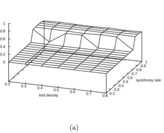
Sampling Surface for ECA146 [50,5000,1000,280676] Avrg 0.2 0.3 0.4 0.5 0.6 0.7 0.8 Intit density 0.2 0.3 0.4 0.5 0.6 0.7 0.8 0.9 1 synchrony rate 0 0.2 0.4 0.6 0.8 1 (a)
Figure 2. An example of sampling surface : ECA 18. The value of the indicators for this surface are ra = 0.03 (no change around α ∼ 1) and rb= 0.19 (important change in the asynchronous domain).
The first parameter is used to measure how small introduction of syn-chrony affects the global behavior of the CA. The small-asynsyn-chrony- small-asynchrony-introductionindicator rais given by :
ra= { 1 |D|
X d∈D
[µexp(d, αas) − µexp(d, 1.0)]2 }1/2 .
This parameter is the quadratic average of the variations of µexp be-tween total synchronism αas= 1.0 − αstpand the highest asynchronous value. It somehow estimates the averaged absolute value of the “jump” of value that can occur for α ∼ 1.
The second parameter is used to measure how the change of syn-chrony from αas to αmin globally affects the behavior of the CA. The asynchrony-dependence indicatorrb is then defined by :
rb= supα∈A′{ 1 |D| X d∈D [µexp(d, α + αstp) − µexp(d, α)]2 }1/2 . with A′= [αmin, αmax− 2.αstp](αstp). This parameter is the maximum quadratic average on dini, for all asynchronous densities, of the varia-tions of µexp. It estimates, in the asynchronous regime, how far from invariance in respect to the translation of axis α the surface is.
2.3.2 Limits of the protocol
Like in any simulation approach, the width of validity for the results we obtain is limited by some of the choices we had to make in the design
of the protocol. Let us try to identify some of these limits.
First, it is clear that our results are limited to the particular region defined by the constants chosen in the experimental protocol. In order to calculate the “observation function”, we have to set the value of the parameters Ttransient and Tsampling. These values are chosen as big as
possible with the implicit assumption that µexp does no longer change
when Ttransientand Tsampling are increased.
Similarly, the choice of the grid size n might influence the outcome of the results. For example, the particular ECA 90 has a transition function that can be expressed in the synthetic form : ∀(a, b, c) ∈ Q3, f (a, b, c) = a ⊕ c with ⊕ denoting the addition modulo 2. The
additivity of the local rule allows a superposition principle to be obeyed by the global rule :
∀(x, x′) ∈ QL× QL, Fsynch(x ⊕ x′) = Fsynch(x) ⊕ Fsynch(x′) .
The evolution of configuration containing a single cell that is in state 1 leads to the formation of Pascal’s Triangle modulo 2. Using the superposition principle, it is easy to see that for grid sizes that are powers of two, n = 2k, k ∈ N, any initial configuration evolves to the
null configuration ¯0in number of step less or equal to n/2. However, for sizes that are not powers of two this nilpotency property does not hold any more and we instead observe cycles whose length are only bounded by 2n (see [13] for a more precise analysis). This simple observation
shows that we should be very careful not to generalize a result obtained on a particular ring size to any ring size. We however conjecture that the experimental data are not dependent on the ring size for most of the ECA rules. The experimental examination of this assumption will be done in the next section for a small number of values of n.
Let us also stress that the protocol associates to a given initial den-sity the same initial configuration which is re-used for different syn-chrony rates. Moreover, we take only one sample for each couple of control parameters (dini, α). Another possibility would consist in
tak-ing several samples for each point and then compute the average of the measured values µexp. However, this averaging effect could be
mislead-ing in the estimation of the model’s robustness : for some particular rules (e.g. shift) it would be possible to have a behavior that varies strongly according to the initial condition chosen but have a stable average. In this work, we choose to say that such a CA is not robust because we are interested in a concept of robustness that characterizes the evolution of a single configuration and not subsets of configurations. This will be further discussed in Section 4.
All these limitations clearly imply that the indicators (ra, rb) and
even the sampling surfaces are far from holding all the information about a model’s behavior. They should instead be considered as a way of making a projection of the huge space of all possible orbits into
the simpler R2 space. They can also be viewed as a first
approxima-tion tool to identify the “non-robust” CA. Indeed, if a perturbaapproxima-tion produces a change in the density distribution then we are allowed to affirm that we are in presence of a change in behavior. The converse is not true since one could easily imagine a situation in which the den-sity distributions would stay stable whereas some other macroscopic parameters would vary. So there are at least two other limitations of the protocol proposed : the first one is that the use of the density induces a compression of information that could introduce biases for behavior estimation, especially when a rule is number conserving (i.e., when its evolution conserves the density). The second one is that we rely on two indicators that are chosen as quantifiers of the regularity of the sampling surfaces using again an approximation. The analysis of experimental results is then a three-level analysis : the first and sec-ond one are qualitative, they consist in the visual examination of the space-time diagrams and the sampling surface. The third one is quan-titative and uses the indicators (ra, rb). These restrictions confirm once
more that this work is just a first step in the study of asynchronous robustness. It aims to give a global view of the landscape in order to show the pertinence of the problem and to identify to some challenging ways to explore.
3. Exhaustive study of the ECA space
In this section, we start by examining the repartition of all ECA into the indicators space, and divide this space into zones. For each zone, we show the sampling surfaces and we examine how the dynamical systems actually evolve by looking at some orbits.
3.1 Repartition of the ECA
The results were obtained with the experimental value for transient time Ttransient= 5000, sampling time Tsampling= 1000, ring size n = 50,
initial density sampling interval D = [0.2, 0.8](0.1), synchrony rate sampling interval A = [0.2, 1.0](0.1). All the experimental data were obtained with a software dedicated to the study of CA robustness [9].
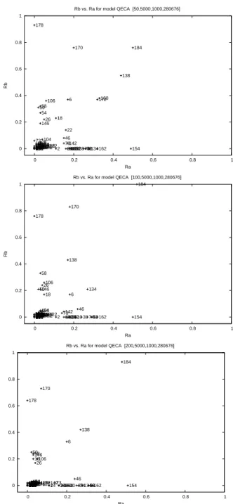
Figure 3 shows the repartition2of the ECA in the 2D space (r a, rb)
for three different values of ring size n. In the three diagrams, the dispersion of the ECA is far from uniform and rather forms groups. If the relative position of the points may vary from one value of n to another, the diagrams appear to have similar distributions. These observation leads us to consider in a first step that the diagram can
2
Recall that only minimal representative ECA have a corresponding point in this space.
0 0.2 0.4 0.6 0.8 1 0 0.2 0.4 0.6 0.8 1 Rb Ra
Rb vs. Ra for model QECA [50,5000,1000,280676]
0 5 3 4 1 2 6 7 8 11 12 13 9 10 14 15 18 19 22 23 25 24 26 27 28 29 30 32 33 35 34 36 37 38 40 41 42 43 45 44 46 50 51 54 56 57 58 60 62 72 73 74 76 77 78 90 94 104 105 106 108 110 122 126 128 132 130 134 136 138 140 142 146 150 152 154 156 160 164 162 168 170 172 178 184 200 204 232 0 0.2 0.4 0.6 0.8 1 0 0.2 0.4 0.6 0.8 1 Rb Ra
Rb vs. Ra for model QECA [100,5000,1000,280676]
0 4 5 3 1 2 6 7 8 9 12 11 13 14 10 15 18 19 22 23 25 24 26 27 28 29 30 32 33 35 36 37 34 38 40 41 42 43 44 45 46 50 51 54 56 57 58 60 62 77 78 72 76 73 74 90 94 104 105 106 108 110 122 126 128 132 130 134 136 138 140 142 146 150 152 154 156 160 164 162 168 170 172 178 184 200 204 232 0 0.2 0.4 0.6 0.8 1 0 0.2 0.4 0.6 0.8 1 Rb Ra
Rb vs. Ra for model QECA [200,5000,1000,280676]
0 5 4 3 1 2 6 7 8 9 11 12 13 14 10 15 18 19 22 23 25 24 26 27 28 29 30 32 33 35 36 37 34 38 40 41 42 43 44 45 46 50 51 57 54 56 58 60 72 62 73 74 76 77 78 90 94 104 105 106 108 110 122 126 128 132 130 134 136 138 140 142 146 150 152 154 156 160 164 162 168 170 172 178 184 200 204 232
Figure 3.Evolution of the repartition in the space (ra, rb) according to different ring sizes : n = 50 (up), n = 100 (middle), n = 200 (bottom); transient and sampling times were : Ttransient= 5000, Tsampling= 1000.
partioned into 4 zones :
In Zone A, we group the ECA that form a dense group in the region defined by ra< 0.1 and rb< 0.1.
In Zone B, we group the ECA that stretch along the ra-axis : ra> 0.1, big rb< 0.1.
In Zone C, we group the ECA that stretch along the rb-axis : ra< 0.1, big rb> 0.1.
In Zone D, we group the other ECA : ra> 0.1, rb> 0.1.
Let us now study each zone separately in order to see if the discrim-ination introduced by the raand rb parameters does allow to separate
the ECA into meaningful classes. For each zone, we examine the shape of the sampling surfaces obtained and try to analyze how this shape is related to the configurations found in the model’s orbits.
3.2 Zone A (small raand small rb)
This zone contains the ECA with high robustness to asynchronism. The models in this zone are situated close to the point (ra, rb) = (0, 0),
this means that given a specific initial condition, the orbits obtained with different synchrony rate produced the same values for the obser-vation function µexp. There can be two straightforward ways to explain
this property :
(H1) The configurations of the asymptotic part (i.e., after the transient time is elapsed) of the orbits are different but the averaging effects used in the experimental protocol produce identical measures for the observation function (see 2.3).
(H2) The configurations of the asymptotic part of the orbit are similar despite having different trajectories during the transient time.
3.2.1 Horizontal surfaces
Rules such as ECA 90 and 150 have been among the most exten-sively studied rules of the ECA space. They are said to be ’additive’ as they obey a superposition principle (see 2.3.2). For these two rules, we found a horizontal sampling surface with µexp∼0.5 for all (dini, α).
This means that the qualitative behavior of the model is invariant when both changing the initial density and the synchrony rate. In-deed, experimental evidence in the synchronous case shows that for any random initial density, the dynamical systems rapidly evolves to-wards an “equilibrium state” for which the density oscillates around ρ = 0.5 [20]. In both synchronous and asynchronous case, this “equilib-rium state” is not a fixed point but is rather a random phase in which the fluctuations of each cell appear to be random (see Figure 4). This
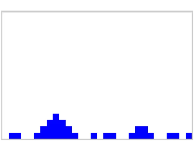
Sampling Surface for QECA90 [ 50,5000,1000,280676] Avrg 0.2 0.3 0.4 0.5 0.6 0.7 0.8 Intit density 0.2 0.3 0.4 0.5 0.6 0.7 0.8 0.9 1 synchrony rate 0 0.2 0.4 0.6 0.8 1 (a) (b)
Figure 4.(a) An example of horizontal surface : ECA 90 (b) Evolution of ECA 90 : (left) α = 1.0 (right) α = 0.5. In this space-time diagram and in the following the intial condition is obtained with a Bernoulli process with dini= 0.5, the grid size is n = 50, the time is from t = 0 to t = 49.
implies that the model’s robustness is explained by H1, more precisely, we expect the distribution of the density after the “transient time” to be a Gaussian with a mean centered around ρ = 0.5 and a variance that is proportional to 1/√n , where n is the lattice size. If this as-sumption is correct, then we have (ra, rb) → (0, 0) as Ttransient → ∞
and Tsampling → ∞, which is what we observed experimentally when
3.2.2 dini-dependent, α-invariant surfaces
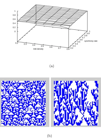
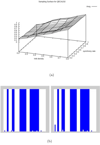
Sampling Surface for QECA232
Avrg 0.2 0.3 0.4 0.5 0.6 0.7 0.8 Intit density 0.2 0.3 0.4 0.5 0.6 0.7 0.8 0.9 1 synchrony rate 0 0.1 0.2 0.3 0.4 0.5 0.6 0.7 0.8 0.9 1 (a) (b)
Figure 5. (a) An example of dini-dependent, α-invariant sampling surface : ECA 232. (b) Evolution of ECA 232 : (left) α = 1.0 (right) α = 0.5. A tight examination of the configuration shows that the width of the second white band is larger in the left diagram.
ECA 232 is an ECA version of the “Majority Vote Rule” : the next state of a cell is the state that it is most present in its neighborhood. We found that this model is a good example of a Zone A ECA with a sampling surface that shows dependence on the initial density dini
and invariance with translation in the α axis : see Figure 5. The dependence on dini is explained by the existence of walls (00 and 11)
created when the dynamical system evolves and we observed a quick convergence of the orbits to a fixed point as seen in Figure 5. This convergence implies that the model’s robustness is explained by H2 as the asymptotic part of the orbits is always a fixed point.
ECA 4, 12, 44, 76 are some others zone A models which showed quick convergence to a fixed point. We can note that for all these mod-els, the local transition rule admits walls3. The question of knowing
how the shape of sampling surface is related to the existence of walls is a potential theoretical problem that arises from these observations and that should be addressed in the future.
3.2.3 Perfectly α-invariant sampling surfaces
Interestingly enough, the analysis of experimental data shows that some ECA are situated exactly on the point (ra, rb) = (0, 0). Their
sampling surface is thus perfectly invariant with translation in the α axis. This means that given a specific initial condition, the choice of the synchrony rate did not influence the value taken by the observation function µexp. The visual examination of the orbits of these
particu-lar ECA shows for a given initial condition, all orbits (for different α) converge to the same fixed point :
∀xi∈ E, ∃xf ∈ QL, ∀α ∈]0, 1], ∃t, γα(xi, t) = xf .
We define the class of “perfectly robust” (PR) CA as the class of models for which the “asymptotic behavior” of a CA is independent of the updating method ∆, with ∆ verifying the fair sampling condition (see 2.1). Some PR rules can be exhibited in a straightforward way. For ECA 0 (null rule), as every cell update turns the cells into state 0, under the fair sampling condition, we are sure to reach the fixed point ¯
0. For ECA 204 (identity), any initial condition is a fixed point and the update does not play any role. If we look at ECA 128 (see Figure 1), all cells turn to state 0 unless they are in state 1 and surrounded by two 0. It is easy to see that the two only fixed points are ¯0and ¯1and that any configuration different from ¯1evolves to the fixed point ¯0.
Experimentally, we find that : PR= { 0, 8, 32, 40, 128, 136, 140, 160, 168, 200, 204 (Identity) }.
To find a sufficient and necessary condition to be in PR is another problem that arises from the analysis of the experimental results.
3.3 Zone B (big ra, small rb)
This zone contains the ECA for which a small introduction of asynchro-nism produces a brutal change of behavior (big ra), while this behavior
no longer changes when asynchronism is increased (small rb).
3
0 and 010 are walls of rule 4, 0 and 01 are walls of rule 12, 00 and 0001are walls of rule 44, 0,01, 10 are walls of rule 76.
3.3.1 Surfaces with a discontinuity at α = 1 and flatness for the rest of the surface
Sampling Surface for QECA2
Avrg 0.2 0.3 0.4 0.5 0.6 0.7 0.8 Intit density 0.2 0.3 0.4 0.5 0.6 0.7 0.8 0.9 1 synchrony rate 0 0.02 0.04 0.06 0.08 0.1 0.12 0.14 0.16 (a) (b)
Figure 6.(a) An example of GAP model sampling surface (z-axis rescaled) : ECA 2. (b) Evolution of ECA 2 : (left) α = 1.0 (right) α = 0.5.
In this zone, we can distinguish some ECA for which we have exactly rb = 0. Visual examination of the sampling surface shows that these
CA exhibit a discontinuity of the surface, indicating a “phase transi-tion” phenomenon, for the points α = 1. When looking at the orbits of these ECA (see Figure 6), we notice that for α = 1, the orbits evolve into a shift-like behavior, where each configuration gets translated by one cell at each time step. For α < 1, the orbits evolve in similar way, except that some “branches” (1-domains) progressively die out. This means that the orbit finally reaches a spatially homogeneous fixed
point consisting in all 0 (the configuration ¯0).
We define GAP as the class of models for which there is a gap in the sampling surface between the values for α = 1 and α < 1 whereas the sampling surface is perfectly horizontal for α < 1. Experimentally, we find that GAP= {2, 10, 24, 34, 42, 56, 74, 130, 154, 162}.
We notice that all ECA in class GAP are “fully asymmetric” (i.e., there are four members in each equivalence class). Moreover, all these rules except 154 are classified as “subshifts” by Cattaneo and al.[3]4.
The asymmetry to the left/right exchange symmetry indicates that the rule has an isotropy which allows a directed propagation of some subwords to happen thus allowing the “subshift” phenomenon in the synchronous mode. On the other hand, the asymmetry to the 0/1 complementation shows that the rules may have a “favorite” state to which to tend to, thus explaining why the attractor ¯0is reached with all the sampled initial conditions in the asynchronous regime.
3.3.2 Surfaces showing a “phase transition” at α = 1 and quasi-flatness elsewhere
For rules 73 and 142, the examination of their sampling surface (Fig-ure 7) showed that an important change of the value of the observation function µexpoccurs for α = 1. On the other hand, in the asynchronous
part (α < 1), the surface appears flat though affected by a little irreg-ularity.
The shape of the surfaces can be explained by the examination of the orbits of the models. As far as the dynamics is concerned, 73 is a border line CA : visual examination of its orbits (see Figure 7) can not clearly help to decide whether it is in Wolfram’s class II (periodic ECA) or in class III (“chaotic” or non-regular ECA) [21]. It is a “Hybrid” (class H) rule according to the classification exposed in [10]. Indeed, when evolved with perfect synchrony the model has a dynamics that is chaotic-like in some parts of the configuration delimited by walls 0110. When a little asynchrony is introduced, there is a non-zero probability that a wall 0110 appears in 0-domains where it was not already present. This means that, as time progresses, more walls appear and the orbit eventually reaches a “quasi-stable state” in which the walls 0110 are separated by three kind of subwords :
0 : these subwords are stable 00 : these subwords are stable
000and 010 : theses two subwords alternate one after another when the update rule is applied in the middle of the word.
4
ECA 154 is symmetric to rule 180 which has been extensively studied in [4] where it was classified as a “generalized subshift” rule. In the classification proposed in [10], the particular behavior of this rule was also noticed as 154 was classified in the “hybrid” (H) class.
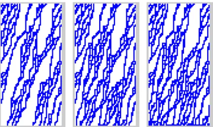
Sampling Surface for QECA73 Avrg 0.2 0.3 0.4 0.5 0.6 0.7 0.8 Intit density 0.2 0.3 0.4 0.5 0.6 0.7 0.8 0.9 1 synchrony rate 0 0.2 0.4 0.6 0.8 1 (a) (b)
Figure 7.(a) An example of surface with a discontinuity at α = 1.0 and noise for α < 1.0 : ECA 73 (z-axis inverted for allowing the display of discontinuity at α = 1). (b) Evolution of ECA 73 : (left) α = 1.0 (right) α = 0.8.
This quick analysis allow us to understand the shape of the sampling surface : the first gap showed by the observation function is due to the appearance of walls when little asynchronism is added, the fluctuations in the surface are due to the random updatings of the 000 and 010 regions. ECA 73 and 142 are the only two elements found in Zone B and that do not belong to class GAP.
Sampling Surface for QECA50 [ 50,5000,1000,280676] Avrg 0.2 0.3 0.4 0.5 0.6 0.7 0.8 Intit density 0.2 0.3 0.4 0.5 0.6 0.7 0.8 0.9 1 synchrony rate 0 0.05 0.1 0.15 0.2 0.25 0.3 0.35 0.4 0.45 0.5 (a) (b)
Figure 8.(a) Sampling surface for an SPT model : 50 (z-axis rescaled). (b) Evolution of ECA 50 : (left) α = 1.0 (center) α = 0.75 (right) α = 0.25.
3.4 Zone C (small ra, big rb)
In this zone, we find the ECA for which an important change of be-havior occurs for values of synchrony rate α < 1.
3.4.1 Surfaces showing a “phase transition” at αc< 1
In Zone C, we find some ECA with a sampling surface which clearly exhibits a discontinuity for a particular value of αc. We have regrouped
this type of models in the class SPT (Single Phase Transition). The analysis of the orbits (see Figure 8) of SPT members showed that for synchrony rates α > αc, the evolution of the space-time
1-domains that evolve on a background of 0. On the other hand, for synchrony rates α < αc, the branching structure quickly dies out and
the orbit reaches the fixed point ¯0. This kind of phenomenon has al-ready been noticed in the study of coupled map lattices and an analogy was made with fluid mechanics : the turbulent phase is represented by the branching structure and the laminar phase is represented by the background of 0 (absorbing state). The laminar phase is stable and can only be destabilized by the diffusion of the turbulent phase. For continuous-state systems, it has been conjectured that the phenomenon of branching structures could be described in terms of directed perco-lation [15]. We are at the moment unable to provide a suitable de-scription for the discrete models, even though the work of Chat´e and Manneville showed that some insight could be gained by understanding CA behavior in terms of discretized coupled map lattices [5], [6].
Experimentally, we find that : SPT= { 6, 18, 26, 50, 58, 106, 146, 178 }.
Note that 22 and 30 have a similar “phase-transition” behavior : in this case, the branching pattern is constituted of defaults of regularity of the regular background 01. This implies that the density of the orbits fluctuates near ρ = 0.5 and that the sampling surfaces are flat and do not allow to detect the qualitative change. ECA 178 has a parameter rb that is much bigger than other SPT members (see Figure 3). This
can be explained by the fact that it is the only member which has two attractors in the stable “phase” (¯0and ¯1), thus producing higher potential changes between the stable phase and the unstable phase.
3.4.2 dini-invariant,α-dependent surfaces
We found that only 126 was in Zone C but not in SPT. 126 is a class III CA ([21]) for which the evolution of the synchrony rate does affect the evolution of the density “smoothly” (see Figure 9).
3.5 Zone D (big ra, big rb)
3.5.1 Unstable surfaces
In this zone, we find the ECA for which the measure of µexp is highly
unstable. When raand rb are high, this can indicate a bad statistical
convergence of the parameters leading to the formation of a non-regular surface (see Figure 10). In these rules, when starting from any initial configuration different from ¯0or ¯1, we see that large zones of 0’s or 1’s appear and the borders of these zones drift in random way until they meet and annihilate. This is the case for ECA 138, 170(shift) and 184.
We notice that ECA 170 and 184 are two (non-trivial) number-conserving ECA in the synchronous case and this suggests that analyt-ical results could be obtained for such simple systems. ECA 138 is a
Sampling Surface for QECA126 Avrg 0.2 0.3 0.4 0.5 0.6 0.7 0.8 Intit density 0.2 0.3 0.4 0.5 0.6 0.7 0.8 0.9 1 synchrony rate 0 0.2 0.4 0.6 0.8 1 (a) (b)
Figure 9. (a) An example of dini-invariant,α-dependent sampling surface : ECA 126 (α-axis inverted). (b) Evolution of ECA 126 : (left) α = 1.0 (center) α = 0.9 (right) α = 0.5.
rule which behavior is similar to 170 with one single difference on the output of the transition function : For (a, b, c) 6= (1, 0, 1) f(a, b, c) = a and f (1, 0, 1) = 0, this implies that the attractor ¯1is unreachable as a consecutive zone of 0 can not disappear.
3.5.2 A Sampling Surface with riddles : ECA 46
The examination of the sampling surface for 46 revealed a surprising phenomenon : “riddles” almost parallel to the dini-axis appear on the
sampling surface (see Figure 11). We conjecture that ECA 46 is a model for which there exists a subset of configurations I ⊂ QL which
Sampling Surface for QECA170 Avrg 0.2 0.3 0.4 0.5 0.6 0.7 0.8 Intit density 0.2 0.3 0.4 0.5 0.6 0.7 0.8 0.9 1 synchrony rate 0 0.2 0.4 0.6 0.8 1 (a) (b)
Figure 10. (a) An example of ill-defined surface : ECA 170 (shift). (b) Evolution of ECA 170 : (left) α = 1.0 (right) α = 0.8.
provide “merging orbits” :
∀(x1, x2) ∈ F × F, ∀α ∈]0, 1], ∃t, γα(x1, t) = γα(x2, t) = xt ,
with the particularity that xtis not a fixed point. This can be observed
in Figure 12 in which α is kept constant and where dini varies.
The very existence of such models is surprising since it implies that different initial conditions eventually merge into the same orbit without even stabilizing on a fixed point. Obviously for ECA 46, I is not strictly equal to QL as ¯0is not part of I (it is a fixed point). However,
Sampling Surface for QECA46 Avrg 0.2 0.3 0.4 0.5 0.6 0.7 0.8 Intit density 0.2 0.3 0.4 0.5 0.6 0.7 0.8 0.9 1 synchrony rate 0.05 0.1 0.15 0.2 0.25 0.3 0.35 0.4 0.45 0.5 0.55 (a) (b)
Figure 11. (a) An example of sampling surface with “riddles” : 46 (α-axis inverted). (b) Evolution of ECA 46 : (left) α = 1.0 (center) α = 0.75 (right) α = 0.25.
conjecture that I = QL− {¯0} meaning that for a fixed dynamics, all
non-zero configuration eventually merge into a single orbit. Such result should be explored in a future work both by experimental and formal approach.
3.5.3 dini-invariant,“U”-shaped surfaces
ECA 6, 38 and 134 have an unexpected behavior : just like GAP the introduction of a little bit of asynchronism makes the system evolve to a homogeneous fixed point. However, unlike SPT ECA, the observation of a long-lived branching structure occurs for values of α smaller than
Figure 12. Evolution of ECA 46 for α = 0.40 and dini = 0.30 (left) 0.50 (center) 0.80 (right)
αc.
ECA 6 sampling surfaces illustrates how GAP-type discontinuity at α = 1 and an SPT-type discontinuity at α ∼ 0.3 (see Figure 13) can both cohabitate. The conjunction of both characteristics explains why this model is situated in zone D (high ra, high rb). It is worth
noticing that the unstable phase (µexp > 0) is obtained for values of
synchrony rates that are lower than the critical value αcand the stable
phase (fixed point ¯0, µexp = 0) is located for α > αc. It implies that the system can become less stable when asynchronism is increased. This observation seems to contradict the thesis proposed in [2] which conjectured that the increase of asynchrony has a stabilizing effect on the dynamics of the models. It shows that a deeper analysis is needed to understand when the increase of asynchrony (i.e., the decrease of α) may stabilize a model by allowing it to reach a fixed point or a stable phase.
4. Discussion
In this paper we described a general-purpose scheme to quantify the robustness of a CA to asynchronism. We chose to observe this ro-bustness according to a protocol which used the density macroscopic parameter and a sampling strategy based on choosing randomly initial conditions and synchrony rates. We have applied this protocol to the 88 equivalence classes of the ECA space to show that a wide variety of phenomena could be observed. In order to go further than the simple visual observation of the orbits we used the sampling surfaces as a
syn-Sampling Surface for QECA6 Avrg 0.2 0.3 0.4 0.5 0.6 0.7 0.8 Intit density 0.2 0.3 0.4 0.5 0.6 0.7 0.8 0.9 1 synchrony rate 0 0.05 0.1 0.15 0.2 0.25 0.3 0.35 0.4 0.45 0.5 (a) (b)
Figure 13.(a) An example of a U-shaped sampling surface : ECA 6. (b) Evolution of ECA 6 : (left) α = 1.0 (center) α = 0.75 (right) α = 0.25.
thetic means of representing a model’s robustness and we proposed two indicators to induce a partial order on the models by quantifying this robustness in R2. This methodology allowed us to induce a distinction
between the different rules of the ECA space and to define robustness classes according to the types of changes that were observed when we added asynchronism in the update rule. We can now discuss our initial questions in two directions : about robustness and about modeling.
4.1 About robustness
An important feature of our classification is that the classes defined according to robustness criteria cannot be deduced from Wolfram’s
empirical classification [21]. For example, if we take the “chaotic” rules, we find that ECA 122 is in Zone A while 18 and 146 are in Zone C (SPT). If we take the “periodic” rules, we find that ECA 232 is in Zone A, 34 is in Zone B (GAP), 50 is in Zone C (SPT), rule 6 is in Zone D (U-shaped). This opens new perspectives for constructing a theory which could predict the shape of the sampling surfaces by analyzing the form of the local transition rule. We proposed the use of walls as a first step in this analysis with the ECA 232 and 73. This classification based on robustness might equally be related with the classification proposed by K˚urka[12]. Indeed, it has been shown that the existence of blocking words allows one to determine the class of an automaton and it appears that walls are just a stronger version of blocking words. It has been recently demonstrated that at least three of the four classes of this classification are undecidable [8] but the question remains open to decide whether a classification based on walls might be decidable and easily computable.
It is important to notice that we never used the fact that the an-alyzed objects were two-state, radius one, one-dimensional CA in the definition of the experimental protocol. This leaves the possibility to explore the behavior of models defined with a higher number of states and in higher dimensions. For two dimensional CA, the study of ro-bustness could be as well examined with respect to changes in the lattice topology. Indeed, one may also want to know whether a small perturbation on the regularity of the lattice may produce significant changes in the behavior of a 2D cellular automaton.
Another possibility of improving the study concerns a finer evalu-ation of the quality of the statistics. In our protocol, the number of initial conditions chosen for the sampling is relatively small (≤ 100) and do not allow us to detect interesting particular subsets of config-urations which may produce different results. This suggests that once a model is declared robust (Zone A), it should be studied for a large number of initial conditions to quantify precisely the fraction of ini-tial conditions for which robustness is observed. This could be done with analytic methods or with an exhaustive experimental study of small (n ≤ 30) ring sizes and would provide further refinements of the classification.
4.2 About complex systems modeling
The experimental method developed here is a first approach that can be used as a guideline to select suitable rules for complex systems modeling with cellular automata. The results presented in this work showed that according to the wide range of phenomena observed when asynchrony is introduced, the use of CA as a modeling tool could take advantage of the classification into robustness zones :
The analysis of Zone A allowed us to find the rules which could be suit-able for modeling : they show stability to the perturbation to asyn-chronism according to some observation function. A strong version of robustness was found in the PR models which obeyed a stronger robustness criterium : for all the initial condition tested, the same asymptotic behavior was reached whatever the value of the synchrony rate. The use of such models may provide a way of building CA-based devices with a behavior strongly tolerant to asynchronism.
The behavior of Zone B models, and particularly the GAP class, sug-gests that their synchronous should be discarded for a real-world ap-plication, except if the purpose of the model is precisely to detect the existence of asynchronism. However, in the asynchronous regime, they appear very stable as the same asymptotics are reached whatever the initial conditions.
Identically, some Zone C rules showed that a brutal change in their behavior could occur for a particular critical value αcof asynchronism. This kind of effect can be undesirable if the modeled phenomenon is not supposed to be synchrony-dependent. On the other hand, one may want such feature to be exhibited by a model. For example, in biol-ogy, it is known that the aggregation of the Dictyostelium Discoidum is triggered when a critical value of starvation is reached. To our knowl-edge, none of the various models (e.g., [16] )proposed yet have been successful in predicting the existence of such a critical value. The ex-planation could be that the release of a chemical component (cAMP) changes the “synchronicity” between cells and that the communication between cells is directed by percolation-like effects that explains why the triggering of the aggregation is sudden. In social sciences, a model used for understanding urban settlement also showed great disparities between the synchronous and asynchronous behavior, the “synchrony rate” here being controlled by the “mobility” (ability to go and live elsewhere) of the agents [7].
The existence of models in Zone D indicate that despite the spatial and temporal averaging we used in the definition of the observation function that quantifies a CA behavior, the outcome of the experiments remained irregular. Such models show that the behavior of an ACA may be simple when evolved synchronously and much more complex with an asynchronous update rule (e.g, the shift).
The phenomenology we observed and the existence of robust CA rules suggests that we can no longer claim that a CA model is not valid because transitions occur too regularly to capture real-world phe-nomena : even though the “real-world cells” might affected by some permanent irregularities (synchronism and/or topology faults) or by noise, a CA model might be robust enough to produce the same out-put when evolved with perturbations. This further suggests that there exists no universal answer to the question of knowing which part of the
interesting behavior of a (classical) CA is due to the synchronism. Each modeling problem should instead be studied with a specific approach and the macroscopic parameters and observation functions used in this work, far from being universal, should be chosen according to what fea-ture of the CA is desired to be robust. For example, one may interested in using a CA with many states to model propagating signals in an ex-citable medium. In this case, one should find the suitable parameters to assess the ability to propagate signals and use these parameters in the robustness assessment.
Acknowledgments
We wish to thank Mats Nordahl (University of G¨oteborg, Sweden) for the stimulating discussions held during the Exystence Thematic Insti-tute, Cristopher Moore (Santa Fe InstiInsti-tute, USA), Marianne Delorme, Jacques Mazoyer, Bertrand Nouvel and Fr´ed´eric Chavanon (ENS Lyon, France) for their advice and reading. The LIP is the parallelism com-puter science laboratory of ENS Lyon; it is associated with the CNRS, the ENS Lyon, the INRIA and the University Claude Bernard Lyon I.
References
[1] Jacques M. Bahi and Sylvain Contassot-Vivier, Stability of fully asyn-chronous discrete-time discrete-state dynamic networks, IEEE Transac-tions on Neural Networks 13 (2002), no. 6, 1353–1363.
[2] H. Bersini and V. Detours, Asynchrony induces stability in cellular au-tomata based models, Proceedings of the 4th International Workshop on the Synthesis and Simulation of Living Systems Artif icialLif eIV (Brooks, R. A, Maes, and Pattie, eds.), MIT Press, July 1994, pp. 382– 387.
[3] G. Cattaneo, E. Formenti, and L. Margara, Topological chaos and cel-lular automata, Celcel-lular Automata - A Parallel model (M. Delorme and J. Mazoyer, eds.), vol. 460, Kluwer Academic Publishers, 1999, pp. 213– 259.
[4] G. Cattaneo and L. Margara, Generalized sub-shifts in elementary cel-lular automata: The ”strange case” of chaotic rule 180, Theorectical Computer Science 201 (1998), 171–187.
[5] H. Chat´e and P. Manneville, Spatio-temporal intermittency in coupled map lattices, Physica D 32 (1988), 409–422.
[6] , Criticality in cellular automata, Physica D 45 (1990), 122. [7] A. Drogoul D. Vanbergue, J-P. Treuil, Modelling urban phenomena with
cellular automata, Advances in Complex Systems 3 (2000), 127–140. [8] Bruno Durand, Enrico Formenti, and Georges Varouchas, On
unde-cidability of equicontinuity classification for cellular automata, Discrete Mathematics and Theoretical Computer Science Proceedings, 2003, pp. 117–128.
[9] Nazim Fat`es, Fiatlux CA simulator in Java, Sources and experimental data available from <http://perso.ens-lyon.fr/nazim.fates>.
[10] , Experimental study of elementary cellular automata dynam-ics using the density parameter, Discrete Mathematdynam-ics and Theoretical Computer Science Proceedings AB (2003), 155–166.
[11] B. A. Huberman and N. Glance, Evolutionary games and computer sim-ulations, Proceedings of the National Academy of Sciences, USA 90 (1993), 7716–7718.
[12] P. Kurka, Languages, equicontinuity and attractors in cellular automata, Ergodic Theory & Dynamical Systems 17 (1997), 417–433.
[13] O. Martin, A. Odlyzko, and S. Wolfram, Algebraic properties of cellular automata, Communications in Mathematical Physics 93 (1984), 219. [14] Martin A. Nowak and Robert M. May, Evolutionary games and spatial
chaos, Nature (London) 359 (1992), 826–829.
[15] Yves Pomeau, Front motion, metastability and subcritical bifurcations in hydrodynamics, Physica D 23 (1986), 3–11.
[16] Nicholas J. Savill and Paulien Hogeweg, Modelling morphogenesis: From single cells to crawling slugs, Journal of Theoretical Biology 184 (1997), 229–235.
[17] Birgitt Sch¨onfisch and Andr´e de Roos, Synchronous and asynchronous updating in cellular automata, BioSystems 51 (1999), 123–143. [18] W. Richard Stark and William H. Hughes, Asynchronous, irregular
au-tomata nets: the path not taken, BioSystems 55 (2000), 107–117. [19] R. L. Buvel T.E. Ingerson, Structure in asynchronous cellular automata,
Physica D 1 (1984), 59–68.
[20] S. Wolfram, Statistical mechanics of cellular automata, Reviews of Mod-ern Physics 55 (1983), 601–644.
[21] , Universality and complexity in cellular automata, Physica D 10 (1984), 1–35.