HAL Id: halshs-00201350
https://halshs.archives-ouvertes.fr/halshs-00201350
Submitted on 22 Jul 2009
HAL is a multi-disciplinary open access archive for the deposit and dissemination of sci-entific research documents, whether they are pub-lished or not. The documents may come from
L’archive ouverte pluridisciplinaire HAL, est destinée au dépôt et à la diffusion de documents scientifiques de niveau recherche, publiés ou non, émanant des établissements d’enseignement et de
A Structural Analysis of the Correlated Random
Coefficient Wage Regression Model
Christian Belzil, Jörgen Hansen
To cite this version:
Christian Belzil, Jörgen Hansen. A Structural Analysis of the Correlated Random Coefficient Wage Regression Model. Econometrics, MDPI, 2007, 140 (2), pp. 827-848. �halshs-00201350�
A Structural Analysis of the Correlated
Random Coe¢ cient Wage Regression Model
1
Christian Belzil
Concordia University, CIRANO, CIREQ and IZA
Jörgen Hansen
Concordia University, IZA and CEPR
February 13, 2004
1An earlier version of this paper was presented at the CIRANO Conference
on the Econometrics of Education: Modeling Selectivity and Outcomes (April, 2002), the ESEM 2002 (Venice, August 2002) and the Canadian Econometric Study Group (October 2002). We thank all seminar participants. Belzil thanks the Social Sciences and Humanities Research Council of Canada for generous funding.
Abstract
We estimate a …nite mixture dynamic programming model of schooling deci-sions in which the log wage regression function is set in a random coe¢ cient framework. We also analyze the determinants of 3 counterfactual experi-ments (a college attendance subsidy, a high school graduation subsidy and an overall decrease in the rate of time preference) and examine a proposition often claimed in the “Average Treatment E¤ects” literature; that the dis-crepancy between OLS and IV estimates of the returns to schooling may be explained by the relatively higher returns experienced by those a¤ected by ex-ogenous policy changes. We …nd that the average return to experience upon entering the labor market (0.0863) exceeds the average return to schooling (0.0576) and we …nd more cross-sectional variability in the returns to expe-rience than in the returns to schooling. Labor market skills (as opposed to taste for schooling) appear to be the prime factor explaining schooling at-tainments. We …nd little evidence in favor of a positive correlation between reactions induced by an exogenous experiment and the individual speci…c returns to schooling.
Key Words: Random Coe¢ cient, Returns to Schooling, Comparative Advantages, Dynamic Programming, Dynamic Self-Selection.
1
Introduction and Objectives
In this paper, we investigate the empirical properties of the correlated random coe¢ cient wage regression model (CRCWRM) using a structural dynamic programming model.1 The term “correlated random coe¢ cient wage regres-sion model”refers to the standard Mincerian log wage regresregres-sion function in which the coe¢ cients may be arbitrarily correlated with the regressors (edu-cation and experience). While the comparative advantages representation of the labor market is far from being new (Roy, 1951, Becker and Chiswick, 1966 and Willis and Rosen, 1979), economists have only recently paid particular attention to the speci…cation and the estimation of linear wage regression models set in a random coe¢ cient framework (Heckman and Vitlacyl (1998, 2000), Wooldridge (1997, 2000), Angrist and Imbens (1994), Card (2000) and Meghir and Palme (2001)). In this recent branch of the literature, it is customary to estimate the log wage regression function using Instrumental Variable (IV) techniques and interpret the estimates in a framework where the returns to schooling are individual speci…c. This surge of new research is understandable. In a context where schooling is understood as the outcome of individual decision making within a dynamic framework, rational individuals base their schooling decisions partly on absolute and comparative advantages in the labor market and partly on their taste for schooling. As a consequence, the random coe¢ cients (the returns to schooling and experience), as opposed to only the individual speci…c intercept terms, will normally be correlated with individual schooling attainments.
In a linear wage regression, individual di¤erences in the intercept term represent a measure of absolute advantage in the labor market while di¤er-ences in slopes re‡ect individual comparative advantages in human capital acquisition via schooling and experience. While it might be tempting to focus solely on heterogeneity in the returns to schooling (and assume homogeneous returns to experience), this approach is likely to be unsatisfactory. If the re-turns to schooling and experience are truly correlated, ignoring individual di¤erences in the return to labor market experience is likely to a¤ect the estimates of the returns to schooling as well as the causal link between labor market ability and schooling (dynamic self-selection). Modeling wage regres-sions in a random coe¢ cient framework therefore requires the allowance for
1The term “correlated random coe¢ cient wage regression model”is also used in
heterogeneity in the returns to experience.2
As it stands, very little is known about the empirical properties of the CR-CWRM. For instance, those interested in estimating the returns to schooling by IV techniques usually ignore higher moments such as the variance of the returns to schooling and experience, or use a reduced-form framework which cannot disclose the covariances between realized schooling and the individ-ual speci…c coe¢ cients. However, these quantities are important. They may shed light on the importance of comparative advantages in the labor market and help comprehend the determinants of individual schooling attainments. Finally, they may help quantify the “Ability Bias” (OLS bias) arising in es-timating the returns to schooling using regression techniques. Obviously, a random coe¢ cient regression model provides a realistic framework to evalu-ate the relative importance of labor markets skills and taste for schooling in explaining cross-sectional di¤erences in schooling attainments. Virtually all recent work on empirical earnings functions is directly or indirectly based on a random coe¢ cient framework. For this reason, it deserves some attention.3
Our main objective is to investigate the empirical properties of the CR-CWRM. These include the population average returns to schooling and ex-perience, the relative dispersions in the returns to schooling and exex-perience, and the relative importance of labor market skills and individual speci…c taste for schooling in explaining cross-sectional di¤erences in schooling at-tainments. We estimate a …nite mixture structural dynamic programming model of schooling decisions with 8 unknown types of individuals, where each type is characterized by a speci…c log wage regression function (linear) as well as a speci…c utility of attending school.4 The estimation of a mixed
2Individual di¤erences in the return to experience may be explained by comparative
advantages in on-the-job training, learning on the job, job search or any other type of post-schooling activities enhancing market wages. Allowing for heterogeneity in the returns to experience is especially important if individual post-schooling human capital investments are unobserved (which is the case in most data sets).
3Heterogenity in realized returns to schooling may also arise if the local returns change
with the level to schooling. In a recent paper, Belzil and Hansen (2002a) used a structural dynamic programming model to obtain ‡exible estimates of the wage regression function from the National Longitudinal Survey of Youth (NLSY). They found that the log wage regression is highly convex and found returns to schooling much lower than what is usually reported in the existing literature although the local returns may ‡uctuate between 1% (or less) and 13% per year.
4In this paper, we disregard using available measures like AFQT scores. We do so
likelihood function has two main advantages. It can capture any arbitrary correlation between any of the heterogeneity components and it obviates the need to incorporate all parents’background variables in each single hetero-geneity component or to select, somewhat arbitrarily, which heterohetero-geneity components are correlated with household background variables and which ones are not.
A second objective is to illustrate the importance of population hetero-geneity and, more speci…cally, to analyze the characteristics of the sub-population (s) most a¤ected by a counterfactual experiment. This is an important issue. In the literature, estimates of the returns to schooling ob-tained using instrumental variable techniques are often higher than OLS estimates.5 It is often postulated that these results are explained by the fact
that those individuals more likely to react to an exogenous policy change must have higher returns to schooling than average. As far as we know, this claim has neither been proved nor veri…ed empirically in any direct fashion. To illustrate the importance of heterogeneity in the reactions to treatment, we conducted 3 counterfactual experiments. We …rst increased the level of the utility of attending school so to mimic the e¤ect of a college subsidy. As this experiment is targeted at speci…c school levels, we also simulated a decrease in the rate of time preference. This experiment is more likely to a¤ect school attendance at all levels, although it is perhaps more di¢ cult to associate an empirical counterpart to it.6 Finally, we simulated a high school
graduation subsidy which, for instance, might be targeted at reducing high school drop out behavior. In all cases, the experiment represents a “truly exogenous” change which may serve as a basis for a natural experiment.
A third and …nal objective is to investigate the notion of “Ability Bias”in a context where the notion is much deeper than the usual correlation between
tests are not taken at the same age by all young individuals). Second, and perhaps more importantly, we are interested in developing a methodology which may be applicable to a wide range of panel data sets. As far as we know, most panel data sets of labor market histories do not contain observed measures of skill heterogeneity such as AFQT scores and the like.
5The validity of very high returns to schooling, reported in a simple regression
frame-work have been seriously questioned (see Manski and Pepper, 2000 and Belzil and Hansen, 2002a). It is also interesting to note that empirical evidence also suggests that standard wage regressions augmented with observable measures of ability (such as test scores and the like) lead to a decrease in the estimated returns to schooling.
6In the literature, it is sometimes argued that di¤erences in credit constraints may be
the individual speci…c intercept terms of the wage regression and realized schooling attainments. As market ability heterogeneity is multi-dimensional in our model, our estimate of the Ability Bias (OLS bias) is not only explained by the correlation between the individual speci…c intercept term and realized schooling but also by the simultaneous correlations between schooling and experience and the individual speci…c deviations from population average returns to schooling and experience.
The model is implemented on a panel of white males taken from the National Longitudinal Survey of Youth (NLSY). The panel covers a period going from 1979 until 1990. The main results are as follows. We …nd pop-ulation average returns to schooling which are much below those reported in the existing literature. Our estimates are also much lower than those obtained using standard OLS techniques. The average return to experi-ence upon entering the labor market (0.0863) exceeds the average return to schooling (0.0576) and we …nd more cross-sectional variability in the returns to experience than in the returns to schooling. The returns to schooling and experience are found to be positively correlated. Not surprisingly, the corre-lated random coe¢ cient wage regression model …ts wage data very well. It can explain as much as 78.5% of the variation in realized wages. Overall, the dynamic programming model indicates that labor market skills are the prime factor explaining schooling attainments as 82% of the explained variation is indeed explained by individual comparative and absolute advantages in the labor market and only 18% is explained by individual di¤erences in taste for schooling. Moreover, realized schooling attainments are more strongly corre-lated with individual di¤erences in returns to experience than in returns to schooling.
The importance of individual heterogeneity in the level of reactions to pol-icy changes is well illustrated by the 3 counterfactual experiments that we conducted. In all cases (the college attendance subsidy, the high school grad-uation subsidy and the overall decrease in the rate of time preference), the reactions induced by the arti…cial instrument are a complicated (non-linear) function of individual speci…c skills and, moreover, the determinants of the reactions will di¤er according to the nature of the experiment. More speci…-cally, it appears that the determinants of the reactions are very much a¤ected by whether or not the experiment is targeted at a particular school level. However, homogeneity is strongly rejected. Unlike what is often claimed in the average treatment e¤ects literature, the discrepancy between IV and OLS is not necessarily explained by a positive correlation between individual
speci…c schooling reactions and the returns to schooling. While it is possible to reconcile our results with conventional wisdom about IV estimates of the returns to schooling in one of our experiments (the general decrease in the discount rate), a positive correlation between individual speci…c reactions and the returns to schooling is not a “general consequence”of any exogenous change in the determinant of school attendance.
The paper is structured as follows. The empirical dynamic programming model is exposed in Section 2. The goodness of …t is evaluated in Section 3. A discussion of the estimates of the return to schooling and experience are found in Section 4. In Section 5, we illustrate the links between labor market skills and dynamic self-selection. In Section 6, we analyze the deter-minants of the individual speci…c reactions to 3 counterfactual experiments and examine a proposition often claimed in the “Average Treatment E¤ects” literature; that the discrepancy between OLS and IV estimates of the returns to schooling may be explained by the relatively higher returns experienced by those a¤ected by exogenous policy changes. In Section 7, we discuss the links between our estimates and those reported in the literature and re-examine the notion of Ability Bias in a context where the regression function allows for a rich speci…cation of absolute and comparative advantages. The conclusion is in Section 8.
2
An Empirical Dynamic Programming Model
of Schooling Decisions with Comparative
Advantages
In this section, we introduce the empirical dynamic programming model. While the theoretical structure of the problem solved by a speci…c agent is similar to the model found in Belzil and Hansen (2002a), the di¤erent stochastic speci…cation and, especially, the allowance for a rich speci…cation of absolute and comparative advantages requires a full presentation.
Young individuals decide sequentially whether it is optimal or not to enter the labor market or continue accumulate human capital. Individuals maximize discounted expected lifetime utility over a …nite horizon T and have identical preferences. Both the instantaneous utility of being in school and the utility of work are logarithmic. The control variable, dit;summarizes
of schooling at the beginning of period t. When dit = 0, an individual
leaves school at the beginning of period t (to enter the labor market). Every decision is made at the beginning the period and the amount of schooling acquired by the beginning of date t is denoted Sit:
2.1
The Utility of Attending School
The instantaneous utility of attending school, Us(:); is formulated as the
following equation7
Us(:) = (Sit) + i + "it (1)
in which "it i:i:d N (0; 2)represents a stochastic utility shock, the term i
represents individual heterogeneity (ability) a¤ecting the utility of attending school and (:) captures the co-movement between the utility of attending school and grade level.
We assume that individuals interrupt schooling with exogenous probabil-ity and, as a consequence, the possibility to take a decision depends on a state variable Iit:8 When Iit = 1; the decision problem is frozen for one
period. If Iit = 0; the decision can be made. When an interruption occurs,
the stock of human capital remains constant over the period.9
2.2
The Utility of Work
Once the individual has entered the labor market, he receives monetary in-come ~wt; which is the product of the yearly employment rate, et; and the
wage rate, wt:The instantaneous utility of work, Uw(:)
Uw(:) = log( ~wt) = log(et wt)
7The utiliy of school could be interpreted as the monetary equivalent (on a per hour
basis) of attending school.
8The interruption state is meant to capture events such as illness, injury, travel,
tem-porary work, incarceration or academic failure.
9The NLSY does not contain data on parental transfers and, in particular, does not
allow a distinction in income received according to the interruption status. As a con-sequence, we ignore the distinction between income support while in school and income support when school is interrupted. In the NLSY, we …nd that more than 85% of the sample has never experienced school interruption.
2.3
The Correlated Random Coe¢ cient Wage
Regres-sion Model
The log wage received by individual i, at time t, is given by
log wit = '1i Sit+ i ('2 Experit+ '3 Exper 2 it) + w i + " w it (2)
where '1i is the individual speci…c wage return to schooling and i is an
individual speci…c factor multiplying the e¤ect of experience ('2) and the
e¤ect of experience squared ('3). The term w
i represents an individual
speci…c intercept term. We assume that
'1i = '1+ !1i
i = + !2i
where '1 and represent population averages. Following the convention
used in the literature, it is convenient to specify the wage regression as a heteroskedastic regression function
log wit = '1 Sit+ '2: Experit+ '3: Exper 2 it+ %it (3) where '2 = '2 '3 = '3 %it = wi + !1i Sit+ !2i ('2 Experit+ '3: Exper 2 it) + " w it
Estimating the population average returns to schooling and experience ('1, '2 and '3 ) is rendered di¢ cult by the fact that typically
Corr( %it; Sit)6= 0
2.4
The Employment Rate
The employment rate, eit; is also allowed to depend on accumulated human
capital (Sit and Experit)so that
ln eit = ln 1 eit = ei + 1 Sit+ 2 Experit + 3 Exper2it+ " e it (4) where e
i is an individual speci…c intercept term, 1 represents the
employ-ment security return to schooling, both 2 and 3 represent the employment
security return to experience.10 The random shock "e
itis normally distributed
with mean 0 and variance 2
e: All random shocks ("it; "wit; "eit)are assumed to
be independent.
2.5
The Value Functions
We only model the decision to acquire schooling beyond 6 years (as virtually every individual in the sample has completed at least six years of schooling). We set T to 65 years and the maximum number of years of schooling to 22. Dropping the individual subscript, the value function associated with the decision to remain in school, given accumulated schooling St , denoted
Vts(St; t);can be expressed as Vts(St; t) = ln( t) + f EVt+1I (St+1; t+1) (5) +(1 ) EM ax[Vt+1s (St+1; t+1); V w t+1(St+1; t+1)]g where VI
t+1(St+1; t+1)denotes the value of interrupting schooling acquisition.
Since we cannot distinguish between income support while in school and income support when school is interrupted, the value of interrupting schooling acquisition is identical to the value of attending school. VI
t+1(St+1; t+1);can be expressed as follows. Vt+1I (St+1; t+1) = log( t+1) + f EV I t+2(St+2; t+2) +(1 ) EM ax[Vt+2s (St+2; t+2); Vt+2w (St+2; t+2)]g (6)
10It follows that the expected value and the variance of the employment rate are given
by Eet= exp( t+12 2
The value of stopping school (that is entering the labor market), Vw
t (St; t),
is given by
Vtw(St; t) = ln(wit eit) + E(Vt+1 j dt= 0) (7)
where E(Vt+1 j dt= 0) is simply
E(Vt+1 j dt= 0) = T X j=t+1 j (t+1) ( exp( j+1 2 2 e)+'1(Sj)+ ['2:Experj+'3:Exper 2 j ])
is simply the expected utility of working from t+1 until T . Using the terminal value and the distributional assumptions about the stochastic shocks, the probability of choosing a particular sequence of discrete choices can readily be expressed in closed form.
2.6
Unobserved Ability in School and in the Labor
Market
We assume that there are K types of individuals. Each type (k) is endowed with a vector ( k; w
k; ek; '1k; k) for k = 1; 2:::K . The results reported in
this paper are for the case K = 8. The probability of belonging to type k; pk; is estimated using logistic transform
pk =
exp(qk) P8
j=1exp(qj)
and with the restriction that q8 = 0.11
2.7
Identi…cation
As it is the case in all empirical dynamic programming models, identi…cation of the key components of the model will require distributional assumption.
11As discussed in Belzil and Hansen (2002a), identi…cation of most parameters is
rela-tively straightforward. However, in order to reduce the degree of under-identi…cation (non-parametric), we …xed the discount rate to 3% per year (an estimate practically identical to the estimate found in Belzil and Hansen (2002a). The degree of under-identi…cation arising in estimating structural dynamic programming models is discussed in details in Rust (1994) and Magnac and Thesmar (2001).
Our model being structured as a single choice dynamic model, data on both wages and schooling attainments allow us to identify the key parameters the utility of attending school (like in Keane and Wolpin, 1997, Eckstein and Wolpin, 1999 and Belzil and Hansen (2002a). Identi…cation of the wage return to schooling, the employment return to schooling and unobserved market ability is relatively straightforward given panel data on labor market wages and employment rates given a distributional assumption about the stochastic shock. In the present case, where the wage regression function may be expressed as a heteroskedastic regression function, identi…cation of the individual speci…c slopes is facilitated by assuming homoskedasticity of the stochastic shocks. However, in order to reduce the degree of under-identi…cation (non-parametric), we …xed the discount rate to 3% per year (an estimate practically identical to the estimate found in Belzil and Hansen (2002a).12
2.8
The Likelihood Function
Constructing the likelihood function (for a given type k) is relatively straight-forward. It has three components; the probability of having spent at most years in school (L1k), the probability of entering the labor market in year
+1;at observed wage w +1 (denoted L2k)and the density of observed wages
and employment rates from + 2until 1990 (denoted L3k): L1k can easily be
evaluated using (5) and (6), while L2k can be factored as the product of a
normal conditional probability times the marginal wage density. Finally L3k
is just the product of wage densities and employment densities. For a given type k, the likelihood is therefore Lk = L1k L2k L3k and the log likelihood
function to be maximized is log L = log 8 X k=1 pk Lk (8)
where each pk represents the population proportion of type k.
12The degree of under-identi…cation arising in estimating structural dynamic
3
Accuracy of Predicted Schooling and
Pre-dicted Wages
Evidence presented in Table 1A shows clearly that the model is capable of …tting the data quite well. A comparison between actual and predicted frequencies reveals that, except for the very low levels of schooling, our model predicts a pattern which is practically identical to the one found in the data. In particular, we are able to predict the large frequencies at 12 years and 16 years. The …t is comparable to what is found in Belzil and Hansen (2001a and 2001b), in which data on household background (parents’education and income, number of siblings and the like) are used explicitly in the utility of attending school as well as in the wage regression.
Using the structural estimates, it is easy to compute a type speci…c ex-pected schooling attainments. These are reported in Table 1B. The type speci…c attainments range from 9.4 years (type 4) to 13.7 years (type 3). An in-depth analysis of the links between schooling and individual speci…c absolute and comparative advantages is delayed to Section 5.
It is also straightforward to use the simulated values of schooling and experience to simulate series of realized lifetime wages. These series can be used to infer the fraction of the variance of realized wages which is explained by the individual speci…c regression functions. To investigate the goodness of …t, we have simulated wages for a cohort of individuals aged 30 in 199013. The
results reported in Table 1C indicate that random coe¢ cient model explains 78.9% of the observed (realized) variation in wages. This is much larger than what is usually reported in the literature, in which standard OLS regressions of wages on schooling and experience typically result in values of R2 ranging
between 0.20 and 0.25 (see Card, 2000).
4
Absolute and Comparative Advantages in
the Labor Market: Some Estimates
In this section, we discuss of the estimates of the return to schooling and experience. The model has been …t on a sample of white males taken from the NLSY and we used the exact same sample as in Belzil and Hansen (2002a).
13We have also simulated wages under various other scenarios and obtained similar
More details are found in Appendix. Note that the estimation of a …nite mixture dynamic programming model not only allows us to estimate the population average returns to schooling and experience but also the cross-sectional variability in the returns. This is a relatively novel feature. As far as we know, no one has ever been able to obtain estimates of the variances of the returns to schooling and experience in a framework where both are endogenous.14
The individual speci…c estimates of the wage regression function (the returns to schooling and experience as well as the individual speci…c intercept terms measuring absolute advantages in the labor market) are found in Table 2A. Our estimates of the returns to schooling range from 0.0265 (type 7) to 0.0879 (type 2) while our estimates of the individual speci…c 0s (ranging from 0.1453 to 1.0866) imply that the returns to experience upon entrance in the labor market range from 0.0197 (type 6) to 0.1477 (type 5). Given the estimates for '2 (0.1359) and '3 (-0.0040), the ordering based on the 0s is identical to the ordering based on the product of and '2 for the most part of the life cycle and, especially, for the early post-schooling period. As an illustration, the individual speci…c returns to experience measured after 8 years of experience (a level higher than the average level of experience measured in 1990) are 0.0719 (type 1), 0.0222 (type 2), 0.0141 (type 3), 0.0191 (type 4), 0.0781 (type 5), 0.0105 (type 6), 0.0690 (type 7) and 0.0246 (type 8).
Overall, and as reported in Belzil and Hansen (2002a), our estimates of the return to schooling are much lower than those reported in the existing literature.15 The population average return to schooling (0.0575) is smaller
than the population average return to experience upon entrance in the labor market (0.0863). Interestingly, the high degree of dispersion in implies a higher standard deviation in the returns to experience (0.0527) than in the returns to education (0.0218). Upon reviewing the estimated 0sand the '01s;
it is also noticeable, although not surprising, that the returns to schooling and experience are positively correlated. The correlation between '1i and i
14Very often, those who focus on the return to schooling use a proxy variable for
experi-ence. Rosenzweig and Wolpin (2000) present a critical analysis of empirical work devoted to the estimation of the returns to schooling, which ignores post-schooling human capital investment.
15However, in Belzil and Hansen (2002a), the wage regression function is estimated
‡exibly using spline techniques. There are 8 di¤erent local returns which range 0.4% per year to 12.0% per year.
is around 0.11 and is discussed in more details below (Section 6). It may be explained by the fact that labor market skills which enhance wage growth (job training, job search, etc..) are positively correlated with academic skills which are rewarded in the labor market. This result has clear impact for the nature of dynamic self-selection. Those endowed with high returns to education will not necessarily obtain a high level of schooling because they will be facing a higher opportunity cost of attending school.
While it is di¢ cult to evaluate the relative degree of heterogeneity in taste for schooling and in the returns to human capital without performing simula-tions, it is nevertheless informative to examine the estimates of the intercept terms of the utility of attending school (reported in Table 2B). Clearly, in-dividual di¤erences in the intercept terms of the taste for schooling appear as important as di¤erences in the intercept terms of the wage equation. The intercept terms for the utility of attending school range from -1.7791 (type 2) to -0.6397 (type 7). Interestingly, even after allowing for 8 types, the high degree of variability (as well as the signi…cance level) of the spline estimates shows that the utility of attending school undoubtedly varies with school level.
Table 3 summarizes the type speci…c rankings according to all hetero-geneity dimensions as well as the level of expected schooling. In an empirical model characterized by a rich speci…cation for skill heterogeneity, the self-selection process is intricate. Individuals take optimal schooling decisions based on their individual speci…c taste for schooling and their absolute and comparative advantages in the labor market. While some individuals are endowed with a high taste for schooling (as can be seen from Table 2B), schooling decisions are largely a¤ected by the combination of comparative advantages (returns to schooling and experience) and absolute advantages (intercept terms of the wage regression). As a consequence, it will be impos-sible to associate a de…nite set of attributes (say, high or low return to human capital) to each speci…c type on the basis of their sole expected schooling at-tainments. Nevertheless, our model is su¢ ciently rich to capture di¤erences in comparative advantages among types of individuals that might obtain similar levels of schooling.
To illustrate this, consider the set of individuals (type 1, type 2, type 4 and type 7) who are predicted to obtain a relatively lower level of schooling than the rest of the population. Type 7 individuals obtain a low level of schooling because they have a low return to schooling and a high return to experience, despite a very high taste for schooling. At the same time, type 2
individuals, who also obtain a low level of schooling, are endowed with high return to schooling and experience. However, these individuals are endowed with a very high wage intercept (high market ability) and a low utility of attending school.
The mechanics of the model can also be illustrated at the higher end of the schooling spectrum. Both type 3 and type 8 individuals are predicted to attain a high level of schooling (13.7 years and 12.6 respectively). While both types face relatively similar returns to schooling and experience, they di¤er substantially in terms of the utility of attending school and the wage intercept. Basically, type 8 individuals choose a high level of schooling be-cause they have a high utility of attending school and type 3 individuals choose a high level of schooling because of a very low level of market abil-ity (wage intercept). A more formal analysis of the link between individual speci…c heterogeneity (comparative advantages) and schooling attainments is performed in the next section.
At this stage, it is informative to examine the estimated correlations be-tween the returns to schooling and other heterogeneity components (taste for schooling, returns to experience and wage intercept). In a standard regres-sion framework where market skill heterogeneity is only intercept based, a positive Ability Bias is easily explained. It arises because the wage intercept term is simultaneously (and positively) correlated with taste for schooling and schooling attainments. However, in the model analyzed therein, self-selection is more complex. The correlation patterns displayed in Table 4 indicate that those who have a high return to schooling also tend to have a high return to experience although the measured correlation (0.1030) is relatively weak. The correlation between the wage intercept and the returns to schooling is also positive (0.2553). This positive correlation indicates that those who tend to have higher wages will also tend to have comparative advantages in schooling and therefore conforms to standard intuition. In-terestingly, taste for schooling is found to be positively correlated with the returns to experience (0.2882) but not with the returns to schooling. The link between these correlations and the treatment e¤ects of an increase in the utility of attending school will be discussed later.
5
Explaining Individual Schooling
Attain-ments: Absolute and Comparative
Advan-tages in the Labor Market vs Taste for
School-ing
To investigate formally the determinants of individual schooling attainments implied by our estimates, we simulated our model and generated 200,000 observations on schooling attainments. Using standard regression techniques, we estimated the e¤ects of each individual speci…c components (taste for schooling, wage intercept, return to schooling and return to experience) on schooling attainments. As the exact form of the relationship between realized schooling and the determinants of the model is unknown, we searched for the best speci…cation. We started by including all elements and their squared terms, and gradually removed all those that were found insigni…cant. We also experimented with log schooling as well as schooling. The resulting regressions are found in Table 5A. To get a better picture of the correlation between schooling and the returns implied by the model, we have plot the returns (average) against each possible schooling levels (Table 5B).
As expected, individual schooling attainments increase with individual speci…c returns to schooling and taste for schooling but decrease with respect to the wage intercept and the return to experience. In total, individual di¤erences in labor market skills and taste for schooling explain 35% of the total cross-sectional variation in schooling. The remaining 65% is explained by pure random wage and utility shocks. When taste for schooling is excluded from the regression (column 2), labor market skills explain 28% of the total variation in schooling attainments. This is interesting. It means that 82% of the explained variations in schooling attainments are explained by labor market skill endowments and only 18% by individual di¤erences in taste for schooling.
While this does not necessarily contradict results recently reported in the literature, it nevertheless o¤ers a di¤erent way of characterizing schooling attainments. For instance, Keane and Wolpin (1997), Eckstein and Wolpin (1999) and Belzil and Hansen (2002a and 2002b) all …nd that individual schooling attainments are largely explained by di¤erences in individual taste for schooling. These di¤erences are either caused by individual abilities or household human capital. However, in all of these papers, individual
di¤er-ences in labor market skills are captured in the intercept term of the wage function. The large e¤ects attributed to di¤erences in the utility of attending school may therefore be explained by the restricted level of heterogeneity in labor market skills.16
6
Skill Heterogeneity and Treatment E¤ects:
An Analysis of 3 counterfactual Experiments
The importance of type speci…c endowments can also be used to learn about the individual speci…c reactions to some “exogenous policy change”. In prac-tice, any “natural experiment” creating changes in the incentives to attend school must e¤ect at least one of the basic components of the decision mak-ing. Therefore, the e¤ect of any exogenous policy change will depend on the fundamental parameters ( k, '1k , wk, k and ).
In the literature concerned with standard linear IV estimation, it is im-plicitly assumed that the induced response is linear in the instrument and that unobserved heterogeneity does not a¤ect treatment. Any departure from these assumptions may have severe consequences. Indeed, the weakness of the IV approach is widely recognized in the treatment e¤ect literature (Card, 2001 and Heckman and Vitlacyl, 1998). As of now, obtaining consistent es-timates of the population average parameters, in a heterogenous treatment e¤ect framework, is still a major challenge.17 Those interested in estimating
average treatment e¤ects using standard IV techniques, often claim that their estimates (which are only valid for a sub-population) are higher than OLS estimates simply because the average returns of the sub-population a¤ected by the instrument are higher than the population average returns (Card, 2000). As far as we know, neither the veracity nor the universality of this claim have been proved nor veri…ed empirically. At this stage, we may only conjecture that the patterns of individual speci…c treatment reactions are
16However, in Keane and Wolpin (1997), the return to schooling varies across broadly
de…ned occupation types. In Belzil and Hansen (2002b), both the utility of attending school and labor market ability are function of household background variables. The au-thors decompose schooling attainments into 2 orthogonal sources, parents’human capital and residual school and market abilities. They …nd that parents’human capital variables are more important than residual ability.
likely to change with the nature of the experiment.18
To illustrate the importance of heterogeneity, we actually conducted 3 counterfactual experiments. We …rst increased the level of the utility of at-tending school so to mimic the e¤ect of a college subsidy. We chose a level of subsidy corresponding to an average of 25% of the per-period utility of attending school so to allow for meaningful changes in schooling.19 As our
objective is only to investigate the level of heterogeneity in the response to treatment, as opposed to obtain a realistic estimate of a college subsidy, the level of the experiment is immaterial. As this experiment is targeted at spe-ci…c school levels, we also simulated a decrease in the rate of time preference (from 0.05 to 0.04). This experiment may be more likely to a¤ect school attendance at all levels, although it is perhaps more di¢ cult to associate an empirical counterpart to it.20 Finally, we simulated a high school graduation
subsidy which, for instance, might be targeted at reducing high school drop out behavior. Nevertheless, in both cases, the experiment represents a “truly exogenous” change which may serve as a basis for a natural experiment.21
6.1
Treatment E¤ects of a Counterfactual College
At-tendance Subsidy
The type speci…c changes in mean schooling following the college attendance subsidy are found in Table 6A. In order to ease the interpretation, we also included the type speci…c mean schooling attainments (from Table 1B) and the returns to schooling (from Table 2A). The results point out to a sub-stantial level of heterogeneity in the reactions to treatment. The average increase is around 2.7 years and the standard deviation is around 2.2. This relatively high average level of reaction is a consequence of the high level of subsidy which we chose. It is informative to examine the mean schooling
18Rosenzweig and Wolpin (2000) discuss a similar argument using a simple theoretical
model of the probability of continuing in high school (the Angrist-Krueger model).
19This subsidy boils down to increase the utility by 0.15.
20In the literature, it is sometimes argued that di¤erences in credit constraints may be
captured in the discount rate (see Cameron and Taber, for a recent example).
21As our model is set in a partial equilibrium framework, this simulations ignore the
potential general equilibrium e¤ects of this policy change and may well exaggerate the e¤ects of treatment. However, as our objective is to examine how various types react to an identical change, the relative reactions are most likely una¤ected by the magnitude of the treatment.
attainments and the returns to schooling of those types that are reacting the most to treatment. Our …nding indicate that the levels of reaction of type 8, type 5 and type 2 individuals are well above the population average. In particular, type 8 individuals (the most a¤ected group) turns out to be com-posed of individuals who are just at the margin of deciding to enter post high school education (12.6 years on average).22 Interestingly, type 8 individuals
are not endowed with a particularly high returns to schooling. Indeed, their return (0.0400) is even below the population average.
To investigate the determinants of the individual speci…c reactions and, in particular, the role of the returns to schooling and experience, we computed OLS regressions of the change in schooling on all measures of skill hetero-geneity. The speci…cation allows for potential non-linearities of the e¤ects of the returns to schooling and experience. The regressions are in Table 6D (columns 1 and 2). The results reported in column 1 (when all heterogeneity components are included) illustrate clearly that the e¤ectiveness of a college subsidy will vary across types. The counterfactual change in years of school-ing decrease with the instantaneous utility of attendschool-ing school ( k);with the level of the wage intercept ( w
k) and with the individual speci…c returns to
schooling ('1k) but increase and the returns to experience ( k) over the
rel-evant range as the 0s vary between 0.20 and 1.08. Obviously, as indicated by the standard errors and the level of R2; a test for the nullity of all slope
parameters (a test for homogeneity of treatment reaction) would be strongly rejected at any reasonable con…dence level.
However, it should be noted that the estimates of Table 6D must be in-terpreted as the marginal e¤ects of each particular heterogeneity component holding other components constant and, as such, are not indicative of the unconditional correlation between the returns to schooling and the individ-ual speci…c reactions to a policy change. Indeed, the results found in column 2 indicate a negative correlation between treatment reaction and the returns to schooling even if we allow for non-linearities (the estimates are -0.0290 and -0.0070). This result does not support the hypothesis that the returns to schooling of those who are more likely to react to an exogenous change in the utility of attending school are overwhelmingly superior to the population average. On the contrary, the returns should be lower.
22Overall, there is a negative correlation between schooling and treatment reaction
6.2
Treatment E¤ects of an Exogenous Decrease in the
Discount Rate
As argued before, a counterfactual decrease in the discount rate (from 0.05 to 0.04) will, by construction, not be targeted at a speci…c school level (say college attendance). For this reason, it may be argued that reaction to treat-ment is less likely to vary across types and more likely to obey the linearity assumption. We can now examine this claim. First, it may be noted from Table 3C that treatment reaction rankings have changed in a non-trivial way. For instance, type 5 individuals are now those who are reacting the most to this counterfactual experiment and they are also endowed with much higher returns to schooling (0.0764) than the population average. As well, the re-gression found in columns 3 of Table 6D indicates that the signs of most of the parameters associated to the determinant of treatment have changed. That is the reaction to treatment increases with the instantaneous utility of attending school ( k) and with the individual speci…c returns to schooling ('1k)but decreases with the level of the wage intercept ( w
k)and the returns
to experience ( k) over the relevant range. However, as in the college
atten-dance subsidy, homogeneity of treatment reaction across types is still strongly rejected although the lower value of R2 indicate that the heterogeneity level
is somewhat less important.
In this experiment, those reacting the most (type 5) appear to have high returns to education so there is hope that the results are compatible with usual claim found in the literature (Card, 2000). Indeed, we …nd that the correlation between the returns to schooling and the reactions to treatment is U shaped when non-linearities are considered. In particular, the parame-ters found in column 4 (-0.44 and 0.04) indicate that at levels of the returns to education above 5.5% per year (virtually the population average return), the positive term will dominate and standard IV estimates will be likely to exceed the population average. In this particular experiment, it is therefore possible to reconcile, at least partially, our results with the common expla-nation advanced for the incidence of very high IV estimates of the returns to schooling.
6.3
Treatment E¤ects of a High School Graduation
Subsidy
As a …nal experiment, we simulated the e¤ects of a 25% increase in the per-period utility of graduating in high school (grade 12). As an example, such an increase could follow from a high school graduation subsidy targeted at reducing the number of high school drop-outs. As in all previous experiments, we present the type speci…c changes in mean schooling following the high school graduation subsidy (Table 6C) as well as the determinants of the individual speci…c treatment reactions (table 6D, columns 5 and 6).
From Table 6C, it may be inferred that type 8 and type 5 individuals are those who will react the most to this policy. Overall, there is a strong resem-blance between the high school graduation subsidy and the college attendance subsidy. While type 5 is composed of high-school drop outs just at the mar-gin of deciding to continue until graduation (their expected level of schooling is 11.5), those types endowed with particularly low level of schooling (type 4 and type 2) do not seem particularly a¤ected by this counterfactual pol-icy. It is also interesting to note that the unconditional relationship between treatment reactions and the returns to schooling has now an inverse U-shape (Table 6D, column 6). Given the parameter values (0.4069 and -0.0496), the negative correlation will however dominate over the range of returns to schooling which exceeds 4% per year. As in the college attendance subsidy, the results of the high school graduation subsidy experiment would not really support the hypothesis that the returns to schooling of those who are more likely to react to are overwhelmingly superior to the population average.
At this stage, it is possible to draw the following 2 conclusions. First, and on a general note, the reactions to policy changes are a complicated non-linear function of individual speci…c attributes. It would be therefore somewhat unnatural to model treatment in a simple linear regression framework unless there is compelling evidence. As pointed out by Rosenzweig and Wolpin (2000), the access to data characterized by a “natural experiment” will not obviate the need to model individual speci…c reactions to treatment. This is exactly what our estimates and simulations indicate.
Second, and more speci…cally, a positive correlation between returns to schooling and the individual speci…c changes in schooling resulting from a policy experiment is far from a “universal”consequence from any exogenous change in the determinants of school attendance. For instance, we …nd no evidence that IV estimates of the returns to schooling arising from the use of
an exogenous subsidy to college attendance as an instrument should lead to particular high returns to schooling (compared to the population average). To the contrary, they should be lower. A practically similar conclusion may be drawn from a high school graduation subsidy.
7
The Correlated Random Coe¢ cient Wage
Regression Model and the Ability Bias
In the existing literature, it is customary to investigate the ability bias indi-rectly by comparing OLS and IV estimates of the return to schooling. Here, the orthogonality of the cross-sectional error term in the CRCWRM may be investigated directly using simulations. Furthermore, in a context where market ability heterogeneity is multi-dimensional, the notion of ability bias is much deeper than the usual correlation between individual speci…c intercept terms of the wage regression and realized schooling attainments. Clearly, the asymptotic OLS bias may be expressed as
As: bias =plim(^ols ) =plim(W
0W N ) 1 plimW0 N where = ('1; '2:; '3)0 W = [St; Expert; Exper2t] N=sample size % = w+ !0 1 St+ !02 ('2 Expert+ '3: Expert2) + "wt .
Note that W is a N x3 matrix of endogenous variables measured at t and that the terms St; Expert; Expert2; %; !1; !2; w are all N x1 vectors.
Obvi-ously, the asymptotic bias will only be equal to 0 if plimWN0 =0. Furthermore, given that the vector of individual speci…c error terms is not centered at 0 and that W0W is not, in general, a diagonal matrix, it is impossible to
ex-press the asymptotic bias in terms of a simple correlation (as in Card, 2000). The components of the vector plimWN0 as well as the resulting bias may easily be computed using the sample created in Section 5. The estimates (along
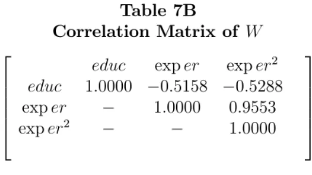
with their p-values) are found in Table 7A. In Table 7B, we also report the correlation matrix of W:
There is clear evidence that accumulated human capital W is not orthog-onal to the error term (Table 7A) and that the degree of non-orthogonality between the vectors of W is important (Table 7B).23The product of the prob-ability limit of the inverse of the moment matrix and the probprob-ability limit of WN0 imply that OLS estimates will over-estimate the return to education and the e¤ect of experience2 and under-estimate the returns to experience. This may be veri…ed easily by estimating the wage regression by OLS us-ing various cross-sections of the NLSY or applyus-ing OLS on the entire panel. Obviously, the OLS estimates for education, experience and experience2 will ‡uctuate according to the speci…c cross-section (year) chosen. To summarize, for the largest cross-sections in the NLSY (88, 89 and 90), the OLS estimate for education will typically ‡uctuate between 8.5% and 10% per year while the returns to experience will be between 3% and 6% per year.
This illustrates another possible explanation for the di¢ culties encoun-tered by those interested in estimating these parameters by IV. In absence of data on entry wages, estimates based on regressions that ignore the endo-geneity of accumulated experience may su¤er serious mis-speci…cation.
8
Conclusion
We have investigated some of the most interesting properties of the corre-lated random coe¢ cient wage regression model using a structural dynamic programming model. In our model, individuals make schooling decisions according to their individual speci…c taste for schooling as well as their indi-vidual speci…c labor market skills and heterogeneity in the realized returns to schooling is interpreted as pure cross-sectional heterogeneity.
We …nd that the average return to experience upon entrance in the labor market (0.0863) exceeds the average return to schooling (0.0576) and we …nd more variability in the returns to experience than in the returns to schooling. The returns to schooling and experience are found to be positively correlated. Not surprisingly, the correlated random coe¢ cient wage regression model …ts
23Rosenzweig and Wolpin (2000) discuss the non-orthogonality between accumulated
experience and ability which may arise when individuals keep optimizing (by choosing the optimal number of hours of work) after having entered the labor market.
wage data very well. It can explain as much as 78.5% of the variation in realized wages.
Interestingly, labor market skills appear to be the prime factor explaining schooling attainments as 82% of the explained variations are indeed explained by individual comparative and absolute advantages in the labor market while 18% only are explained by di¤erences in taste for schooling. Moreover, re-alized schooling attainments are more strongly correlated with individual di¤erences in returns to experience than in returns to schooling.
Our results indicate that the reactions to counterfactual policy changes di¤er substantially across types and that, as a consequence, the usage of natural experiments will not obviate the need for modeling reaction to treat-ment. Furthermore, the characterization of the individual speci…c reactions di¤er substantially according to the nature of the experiment. For instance, a college attendance subsidy and a experiment which would result in a decrease in the discount rate would have very di¤erent consequences, although in both cases, homogeneity of the reaction is rejected. However, as indicated by our results, a positive correlation between returns to schooling and reactions to treatment is not a “universal”consequence from any exogenous change in the determinants of school attendance. For instance, we …nd no evidence that IV estimates of the returns to schooling using a subsidy to college attendance (or a high school graduation subsidy) as an instrument should lead to particular high returns to schooling (compared to the population average).
Finally, the evidence presented in this paper is in accordance with the results presented in Belzil and Hansen (2002a). Although, in the current paper, heterogeneity in the returns to schooling are interpreted as purely cross-sectional and the returns do not change with schooling level, our esti-mates are still much smaller than those reported in the literature. Altogether, the results reported therein, along with those reported in a companion paper, point out to the complexities involved in estimating the returns to schooling. The wage regression function is perhaps a highly non-linear (convex) func-tion and the degree of convexity most likely depends on individual speci…c comparative advantages. At this stage, it is impossible to say whether skill heterogeneity is more important than non-linearities. Only further work will clarify this rather fundamental issue.
References
[1] Angrist, Joshua and Alan B. Krueger (1991) “Does Compulsory School Attendance A¤ect Schooling and Earnings” Quarterly Journal of Eco-nomics”, 106, 979-1014.
[2] Becker, Gary and B. Chiswick (1966) “Education and the Distribution of Earnings” American Economic Review, 56, 358-69.
[3] Belzil, Christian and Hansen, Jörgen (2002a) “Unobserved Ability and the Return to Schooling”, Econometrica, vol 70, 575-591.
[4] Belzil, Christian and Hansen, Jörgen (2002b) “Structural Estimates of the Intergenerational Education Correlation”, forthcoming in Journal of Applied Econometrics.
[5] Cameron, Stephen and Heckman, James (1998) ”Life Cycle Schooling and Dynamic Selection Bias: Models and Evidence for Five Cohorts of American Males” Journal of Political Economy, 106 (2), 262-333. [6] Cameron, Stephen and Chris Taber (2002) “”forthcoming in Journal of
Political Economy
[7] Card, David (2001) “The Causal E¤ect of Education on Earnings”Hand-book of Labor Economics, edited by David Card and Orley Ashenfelter, North-Holland Publishers..
[8] Eckstein, Zvi and Kenneth Wolpin (1999) “Youth Employment and Aca-demic Performance in High School”, Econometrica 67 (6,)
[9] Florens, Jean-Pierre, James Heckman, Costas Meghir and Edward Vyt-lacil (2002) “ Instrumental Variables, Local Instrumental Variables, and Control Functions” working Paper.
[10] Heckman, James and E. Vytlacil (1999) “Local Instrumental variables and Latent Variable Models for Identifying and Bounding Treatment Ef-fects”, Working paper, Department of Economics, University of Chicago. [11] Heckman, James and E. Vytlacil (2000) “Instrumental Variables Meth-ods for the Correlated Random Coe¢ cient Model”, Journal of Human Resources, Volume 33, (4), 974-987.
[12] Imbens, Guido and J. Angrist (1994) “Identi…cation and Estimation of Local Average Treatment E¤ects”, Econometrica, 62, 4,467-76.
[13] Keane, Michael P. and Wolpin, Kenneth (1997) ”The Career Decisions of Young Men” Journal of Political Economy, 105 (3), 473-522.
[14] Magnac, T. and D. Thesmar (2001): “Identifying Dynamic Discrete Decision Processes,” forthcoming in Econometrica.
[15] Manski, Charles and John Pepper (2000) “Monotone Instrumental Vari-ables: with an Application to the Returns to Schooling”Econometrica, 68 (4), 997-1013
[16] Meghir, Costas and Marten Palme (2001) “The E¤ect of a Social Ex-periment in Education” Working Paper, UCL.
[17] Rosenzweig Mark and K.Wolpin (2000) “Natural Natural Experiments in Economics” Journal of Economic Literature, December, 827-74. [18] Roy, Andrew “Some thoughts on the Distribution of Earnings” Oxford
Economic Papers, vol 3 (June), 135-146.
[19] Rust, John (1994) “Structural Estimation of Markov Decision Processes” in Handbook of Econometrics, ed. by R. Engle and D. Mc-Fadden. Amsterdam; Elsevier Science, North-Holland Publishers, 3081-4143.
[20] Sauer, Robert (2001) “Education Financing and Lifetime Earnings” Working Paper, Brown University.
[21] Taber, Christopher (1999) “The Rising College Premium in the Eighties: Return to College or Return to Unobserved Ability”, forthcoming in Review of Economic Studies.
[22] Willis, R. and S. Rosen (1979) “Education and Self-Selection”, Journal of Political Economy, 87, S-7-S36.
[23] Wooldridge, Je¤rey M.(2000) “Instrumental Variable Estimation of the Average Treatment E¤ect in the Correlated Random Coe¢ cient Model”, Working Paper
[24] Wooldridge, Je¤rey M. (1997) “On Two-Stage Least Squares estima-tion of the Average Treatment E¤ect in a Random Coe¢ cient Model”, Economic Letters (56): 129-133.
Table 1A
Model Fit: Actual vs Predicted Schooling Attainments
Grade Level Predicted (%) Actual (%)
Grade 6 0.0% 0.3 % Grade 7 1.4% 0.6% Grade 8 3.4% 2.9% Grade 9 5.4% 4.7% Grade10 6.2% 6.0 % Grade11 7.5% 7.5 % Grade12 38.4% 39.6 % Grade13 7.5% 7.0 % Grade14 5.7% 7.7 % Grade15 2.7% 2.9 % Grade16 12.5% 12.9 % Grade17 2.2% 2.5 % Grade18 2.7% 2.4% Grade19 2.0% 1.3% Grade 20+ 1.1% 1.6%
Table 1B
Mean Schooling and Type Probabilities
Expected Type qk
Schooling Probabilities (pk) (st. error)
type 1 10.81 years 0.1375 -0.0122 (0.0895) type 2 10.43 years 0.0607 -0.8299 (0.0243) type 3 13.69 years 0.0951 -0.3808 (0.0314) type 4 9.41 years 0.0725 -0.6519 (0.0371) type 5 11.51 years 0.1630 0.1579 (0.0577) type 6 10.86 years 0.1260 -0.0992 (0.0584) type 7 10.57 years 0.2059 0.3916 (0.0760) type 8 12.56 years 0.1392 0.0000 (normalized)
Note: The type probabilities are computed using a logistic transforms;
pk =
exp(qk) P8
j=1exp(qj)
Table 1C
Model Fit: Actual vs Predicted Wages
Variance of log 0.9597 predicted wages
variance of log 1.2164 realized wages
Explained Variance (%) 78.9%
Note: Log wages are generated under the assumption that all individuals are aged 30.
Table 2A
Absolute and Comparative Advantages in the Labor Market
Parameter (st. error)
Wages Employment
Type Inter. Educ. Experience Inter.
w i '1i i i '2 i '3 0i 1 1.5325 0.0858 1.0000 0.1359 -0.0040 -3.5753 (0.0308) (0.0052) - (0.0059) (0.0002) (0.0363) 2 1.5664 0.0879 0.3085 0.0419 -0.0012 -2.1070 (0.0153) (0.0050) (0.0409) (0.0213) 3 1.3699 0.0486 0.1958 0.0266 -0.0008 -1.5369 (0.0132) (0.0032) (0.0464) (0.0218) 4 1.8741 0.0595 0.2661 0.0362 -0.0011 -3.7817 (0.0321) 0.0040) (0.0474) (0.0296) 5 1.2028 0.0764 1.0866 0.1477 -0.0043 -3.4752 (0.0401) 0.0037) (0.0472) (0.0286) 6 1.5551 0.0629 0.1453 0.0197 -0.0006 -3.6752 (0.0206) (0.0041) (0.0447) (0.0369) 7 1.3622 0.0265 0.9602 0.1305 -0.0038 -3.4810 (0.0260) (0.0028) (0.0488) (0.0464) 8 1.2539 0.0400 0.3417 0.0464 -0.0014 -3.3763 (0.0156) (0.0031) (0.0352) (0.0400) ave. 1.4190 0.0576 0.6347 0.0863 -0.0025 -3.2559 S.d. 0.1810 0.0218 0.3878 0.0527 0.0016 0.6623
Note: .The estimates of the log inverse employment rate equation are -0.0623 (education), -0.0145 (experience) and 0.0001 (experience squared). The interruption probability is around 7% per year and the log likelihood is -13.7347.
Table 2B
Param. (st. error)
grade level Spline Type Intercept
(:) ( ) grade 7-9 0.0164- Type 1 -1.1296 (0.0080) (0.0540) grade 10 0.3665- Type 2 -1.7791 (0.0142) (0.0922) grade. 11 -1.0540- Type 3 -1.4172 (0.0203) (0.0384) grade 12 1.0894 Type 4 -0.8234 (0.0165) (0.0550) grade 13 -0.5309 Type 5 -1.2595 (0.0165) (0.0487) grade 14 0.5049 Type 6 -1.1255 (0.0159) ( 0.0424) grade 15 -0.8824 Type 7 -0.6397 (0.0196) (0.0326) grade 16 0.9443 Type 8 -0.9934 (0.0242) (0.0548) grade 17- -0.8023 -(0.0223)
Table 3
Absolute and Comparative Advantages: Type Speci…c Rankings
Rankings
Schooling Labor Market
Wages Employment Predicted inter. Intercept return to return to intercept Schooling (abs. adv.) Education Experience term
w ' 1 0 type 1 5 5 4 2 2 3 type 2 7 8 2 1 5 7 type 3 1 7 5 6 7 8 type 4 8 2 1 4 6 1 type 5 3 6 8 3 1 5 type 6 4 4 3 5 8 2 type 7 6 1 6 8 3 4 type 8 2 3 7 7 4 6
Note: To compute the average return to experience, we used the return at 8 years of experience.
Table 4
Correlations between various heterogeneity components
Correlations
wage returns to returns to taste for intercept schooling experience schooling
wage 1.000 0.2553 -0.4098 0.0272 intercept returns - 1.0000 0.1030 0.7175 to schooling returns to - - 1.000 0.2882 experience taste for - - - 1.000 schooling
Table 5A
Estimates of the E¤ects of Labor Market Skills and Taste for Schooling on Schooling Attainments
Parameter (st. error) (1) (2) (3) (4) (5) intercept 4.6112 3.0602 1.9745 2.4369 2.1898 (0.0844) (0.0254) (0.0038) (0.0011) (0.0030) w i -0.4317 -0.2286 - -(0.0630) (0.0337) ( w i )2 -0.1611 -0.0726 - -(0.0173) (0.0113) '1i 100 0.1096 0.0065 - -0.0049 0.0978 (0.0024) (0.0003) (0.0002) (0.0012) ('1i 100)2 -0.0091 (0.0001) i -0.3422 -0.1130 - -(0.0029) (0.0002) 0i 0.2344 0.0395 - -(0.0016) (0.0007) i 0.7743 - -0.7035 -(0.0214) (0.0069) ( i)2 -0.0569 - -0.2582 -(0.0031) (0.0031) R2 0.3452 0.2821 0.0929 0.0042 0.0464
Note: The regressions are performed on 200,000 simulated observations. The dependent variable is log schooling and, for convenience, the returns to schooling and experience are multiplied by 100. Similar results may be obtained using schooling (instead of log schooling).
Table 5B
Average Returns to Schooling by Grade Level Achieved
Grade level Average Returns St. Deviation
6 0.0464 0.0164 7 0.0473 0.0180 8 0.0489 0.0202 9 0.0534 0.0230 10 0.0609 0.0239 11 0.0607 0.0225 12 0.0592 0.0211 13 0.0547 0.0189 14 0.0502 0.0160 15 0.0461 0.0102 16 0.0445 0.0059 17 0.0443 0.0048 18 0.0442 0.0045 19 0.0423 0.0040
Table 6A
A Type Speci…c Analysis of the E¤ects of a Counterfactual College Attendance Subsidy
in Schooling in Schooling returns to Pred. schooling (per type) (ranking) schooling
Type 1 1.7 years 7 0.0858 10.8 years
Type 2 3.0 years 3 0.0879 10.4 years
Type 3 2.8 year 5 0.0486 13.7 years
Type 4 1.4 years 8 0.0595 9.4 years
Type 5 3.3 years 2 0.0764 11.5 years
Type 6 2.5 years 6 0.0629 10.9 years
Type 7 2.9 years 4 0.0265 10.6 years
Type 8 3.16 years 1 0.0400 12.6 years
average 2.7 years - 0.0576 11.8 years (st. dev) (2.2) (0.0218)
Table 6B
A Type Speci…c Analysis of the E¤ects of a counterfactual change in the discount rate
in Schooling in Schooling returns to Pred. Schooling (per type) (ranking) schooling
Type 1 2.1 years 2 0.0858 10.8 years
Type 2 0.7 years 8 0.0879 10.4 years
Type 3 1.31 year 6 0.0486 13.7 years
Type 4 1.0 years 7 0.0595 9.4 years
Type 5 2.6 years 1 0.0764 11.5 years
Type 6 1.4 years 5 0.0629 10.9 years
Type 7 1.9 years 3 0.0265 10.6 years
Type 8 1.4 years 4 0.0400 12.6 years
average 1.7 years - 0.0576 11.8 years (st. dev) (2.3) (0.0218)
Table 6C
A Type Speci…c Analysis of the E¤ects of a High School Graduation Subsidy
in Schooling in Schooling returns to Pred. Schooling (per type) (ranking) schooling
Type 1 0.0 years 8 0.0858 10.8 years
Type 2 1.3 years 6 0.0879 10.4 years
Type 3 1.7 year 3 0.0486 13.7 years
Type 4 0.0 years 7 0.0595 9.4 years
Type 5 1.9 years 2 0.0764 11.5 years
Type 6 1.4 years 5 0.0629 10.9 years
Type 7 1.5 years 4 0.0265 10.6 years
Type 8 1.4 years 1 0.0400 12.6 years
average 1.33 years - 0.0576 11.8 years (st. dev) (2.2) (0.0218)
Table 6D
The determinants of the individual speci…c reactions to a college attendance subsidy and a change in discount rate
Parameter (st. error)
College attendance Decrease in High school subsidy discount rate graduation subsidy (1) (2) (3) (4) (5) (6) intercept -8.2350 3.2170 7.2156 2.6480 -6.6068 0.8667 (0.8536) (0.0420) (0.4835) (0.0450) (0.4425) (0.0422) w i -0.1135 - -2.2556 - -0.7002 -(0.3859) (0.1168) (0.1062) '1i 100 -0.1675 -0.0290 0.3582 -0.4430 -0.3168 0.4069 (0.0405) (0.0025) (0.0361) (0.0180) (0.0329) (0.0166) ('1i 100)2 -0.0542 -0.0070 -0.0069 0.0431 -0.0441 -0.0496 (0.0036) (0.0010) (0.0039) (0.0020) (0.0036) (0.0015) i 6.8437 - -3.4167 1.3485 (0.0029) (0.2721) (0.2482) 2 i -4.3433 3.0235 -0.3044 (0.1656) (0.1790) (0.1633) 0i -1.4679 - 0.3349 -1.4048 (0.0638) (0.0348) (0.0316) i -6.9336 - 2.3425 -6.6557 (0.1640) (0.1783) (0.1616) R2 0.0977 0.0125 0.0524 0.0112 0.1307 0.0288
Table 7A
Estimating the Asymptotic Bias
Estimate (P. Value)
plimWN0 plim(^ols )
Education 6.04 0.04 (0.01) (0.01) Experience 2.09 -0.03 (0.01) (0.01) Experience2 15.27 0.0013 (0.01) (0.01)
Note: The OLS estimates for education, experience and experience2 will
‡uctuate according to the speci…c cross-section (year) chosen. The OLS estimate for education will typically lie between 8% and 10% per year while the returns to experience will be between 3% and 6% per year.
Table 7B Correlation Matrix of W 2 6 6 6 6 4
educ exp er exp er2
educ 1:0000 0:5158 0:5288 exp er 1:0000 0:9553 exp er2 1:0000 3 7 7 7 7 5
Appendix 1 The Data
The sample used in the analysis is extracted from the 1979 youth cohort of the T he N ational Longitudinal Survey of Y outh ( NLSY). The NLSY is a nationally representative sample of 12,686 Americans who were 14-21 years old as of January 1, 1979. After the initial survey, re-interviews have been conducted in each subsequent year until 1996. In this paper, we restrict our sample to white males who were age 20 or less as of January 1, 1979. We record information on education, wages and on employment rates for each individual from the time the individual is age 16 up to December 31, 1990.
The original sample contained 3,790 white males. However, we lacked in-formation on family background variables (such as family income as of 1978 and parents’ education). We lost about 17% of the sample due to missing information regarding family income and about 6% due to missing informa-tion regarding parents’ educainforma-tion. The age limit and missing informainforma-tion regarding actual work experience further reduced the sample to 1,710.
Descriptive statistics for the sample used in the estimation can be found in Table 1. The education length variable is the reported highest grade com-pleted as of May 1 of the survey year and individuals are also asked if they are currently enrolled in school or not.24 This question allows us to identify
those individuals who are still acquiring schooling and therefore to take into account that education length is right-censored for some individuals. It also helps us to identify those individuals who have interrupted schooling. Over-all, the majority of young individuals acquire education without interruption. The low incidence of interruptions (Table 1) explains the low average number of interruptions per individual (0.22) and the very low average interruption duration (0.43 year) . In our sample, only 306 individuals have experienced at least one interruption. This represents only 18% of our sample and it is along the lines of results reported in Keane and Wolpin (1997).25 Given the
age of the individuals in our sample, we assume that those who have already started to work full-time by 1990 (94% of our sample), will never return to school beyond 1990. Finally, one notes that the number of interruptions is
24This feature of the NLSY implies that there is a relatively low level of measurement
error in the education variable.
25Overall, interruptions tend to be quite short. Almost half of the individuals (45 %)
who experienced an interruption, returned to school within one year while 73% returned within 3 years.