Automatic Generation of FPGA-Specific Pipelined Accelerators

HAL Id: ensl-00549682

https://hal-ens-lyon.archives-ouvertes.fr/ensl-00549682

Submitted on 22 Dec 2010

HAL is a multi-disciplinary open access

archive for the deposit and dissemination of

sci-entific research documents, whether they are

pub-lished or not. The documents may come from

teaching and research institutions in France or

abroad, or from public or private research centers.

L’archive ouverte pluridisciplinaire HAL, est

destinée au dépôt et à la diffusion de documents

scientifiques de niveau recherche, publiés ou non,

émanant des établissements d’enseignement et de

recherche français ou étrangers, des laboratoires

publics ou privés.

Automatic Generation of FPGA-Specific Pipelined

Accelerators

Christophe Alias, Bogdan Pasca, Alexandru Plesco

To cite this version:

Christophe Alias, Bogdan Pasca, Alexandru Plesco.

Automatic Generation of FPGA-Specific

Pipelined Accelerators. International Symposium on Applied Reconfigurable Computing (ARC’11),

Mar 2011, Belfast, United Kingdom. �ensl-00549682�

Automatic Generation of FPGA-Specific Pipelined

Accelerators

LIP Research Report RR2010-37

Christophe Alias, Bogdan Pasca, Alexandru Plesco

46 all´ee d’Italie, 69364 Lyon Cedex 07, France Email:{Firstname.Lastname}@ens-lyon.fr

Abstract—Recent increase in the complexity of the circuits has brought high-level synthesis tools as a must in the digital circuit design. However, these tools come with several limitations, and one of them is the efficient use of pipelined arithmetic operators. This paper explains how to generate efficient hardware with pipelined operators for regular codes with perfect loop nests. The part to be mapped to the operator is identified, then the program is scheduled so that each operator result is available exactly at the time it is needed by the operator, keeping the operator busy and avoiding the use of a temporary buffer. Finally, we show how to generate the VHDL code for the control unit and how to link it with specialized pipelined floating-point operators generated using open-source FloPoCo tool. The method has been implemented in the Bee research compiler and experimental results on DSP kernels show promising results with a minimum of 94% efficient utilization of the pipelined operators for a complex kernel.

I. INTRODUCTION

Application development is moving towards packing more features per product. In order to cope with competition, added features usually employ complex algorithms, making full use of existing processing power. When application performance is poor, one may envision accelerating the whole application or a computationally demanding kernel using the following solu-tions: (1) multi-core general purpose processor (GPP): may not accelerate non-standard computations (exponential, logarithm, square-root) (2) application-specific integrated circuit (ASIC): the price tag is often too big, (3) Field Programmable Gate Array (FPGA): provide a balance between the performance of ASIC and the costs of GPP.

FPGAs have a potential speedup over microprocessor sys-tems that can go beyond two orders of magnitude, depend-ing on the application. Traditionally, such accelerations are believed to be obtained only using low-abstraction languages such as VHDL or Verilog taking advantage of the specificity of the deployment FPGA. However, designing entire systems using these languages is tedious and error-prone.

In order to address the productivity issue, much research has focused on high-level synthesis (HLS) tools [22], [2], [9], [1], [7], which input the system description in higher level language, such as C programming language (C). Unfortunately, so far none of these tools come close to the speedups obtained by manual design. Moreover, these tools have important data type limitations.

In order to take advantage of the hardware carry-chains (for performing fast additions) and of the Digital Signal Processing (DSP) blocks (for performing fast multiplications) available in modern FPGAs, most HLS tools use fixed-point data types for which the operations are implemented using integer arithmetic. Adapting the fixed-point format of the computations along the datapath is possible, but requires as much expertise as expressing the computational kernel using VHDL or Verilog for a usually lower performance kernel. Keeping the same fixed-point format for all computations is also possible, but in this case either the design will overflow/underflow if the format is too small, either will largely overestimate the optimal circuit size when choosing a large-enough format.

For applications manipulating data having a wide dy-namic range, HLS tools supporting standard floating-point precisions [9], or even custom precisions can be used [1]. Floating-point operators are more complex than their fixed-point counterparts. Their pipeline depth may count tens of cycles for the same frequency for which the equivalent fixed-point operator require just one cycle. Current HLS tools make use the pipelined FP operators cores in a similar fashion as for combinatorial operators, but employing stalling whenever feedback loops exists. This severely affects performance.

In this paper, we describe an automatic approach for syn-thesizing a specific but wide class of applications into fast FPGA designs. This approach accounts for the operator’s pipeline depth and uses state of the art code transformation techniques for scheduling computations in order to avoid pipeline stalling. We present here two classic examples: matrix multiplication and the Jacobi stencil for which we describe the computational kernels, code transformations and provide synthesis results. For these applications, simulation results show that our scheduling is within5% of the best theoretical pipeline utilization.

II. RELATEDWORK

In the last years, important advances have been made in the generation of computational accelerators from higher-level of abstraction languages. Many of this languages are usually but not limited to C-like subsets with additional extensions. The more restrictive the subset is, the more limited is the number of applications can be synthesized.

For example, Spark [20] can only synthesize integer datatypes. This is unfortunate, as the application class requir-ing only integer computations is very narrow.

Tools like Gaut [22], Impulse-C [2], Synphony [7] require the user to convert the floating-foint (FP) specification into a user-defined fixed-point format. Other, like Mentor Graphics’ CatapultC [5], claim that this conversion is done automatically. Either way, without additional knowledge on the ranges of processed data, the determined fixed-point formats are just estimations. Spikes the input data can cause overflows which invalidate large volumes of computations.

In order to workaround the known weaknesses of fixed-point arithmetic, AutoPilot [9] and Cynthesizer [1] (in SystemC) can synthesize FP datatypes by instantiating FP cores within the hardware accelerator. AutoPilot can instantiate IEEE-754 Single Precision (SP) and Double Precision (DP) standard FP operators. Cynthesizer can instantiate custom precision FP cores, parametrized by exponent and fraction width. Moreover, the user has control over the number of pipeline stages of the operators, having an indirect knob on the design frequency. Using this pipelined operators requires careful scheduling techniques in order to (1) ensure correct computations (2) prevent stalling the pipeline for some data dependencies. For algorithms with no data dependencies between iterations, it is indeed possible to schedule one operation per cycle, and after an initial pipeline latency, the arithmetic operators will output one result every cycle. For other algorithms, these tools manage to ensure (1) at the expense of (2). For example, in the case of algorithms having inter-iteration dependencies, the scheduler will stall successive iterations for a number of cycles equal to the pipeline latency of the operator. As said before, complex computational functions, especially FP, can have tens and even hundreds of pipeline stages, therefore significantly reducing circuit performance.

In order to address the inefficiencies of these tools regarding synthesis of pipelined (fixed or FP) circuits, we present an automation tool chain implemented in the Bee research com-piler [8], and which uses FloPoCo [16], an open-source tool for FPGA-specific arithmetic-core generation, and advanced code transformation techniques for finding scheduling which minimize pipeline stalling, therefore maximizing throughput.

III. FLOPOCO-A TOOL FOR GENERATING COMPUTATIONAL KERNELS

Two of the main factors defining the quality of an arith-metic operator on FPGAs are its frequency and its size. The frequency is determined by the length of the critical path – largest combinatorial delay between two register levels. Faster circuits can be obtained by iteratively inserting register levels in order to reduce the critical path delay. Consequently, there is a strong connection between the circuit frequency and its size.

Unlike other core generators [3], [4], FloPoCo takes the target frequency f as a parameter. As a consequence, com-plex designs can easily be assembled from subcomponents generated for frequency f . In addition, the FloPoCo operators

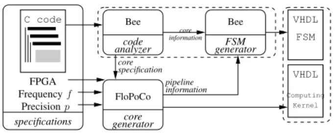
FloPoCo Bee Bee generatorcore generatorFSM core specification FPGA Frequencyf Precisionp specifications C code analyzercode core information information pipeline VHDL FSM VHDL Kernel Computing

Fig. 1. Automation flow

are also optimized for several target FPGAs (most chips from Altera and Xilinx), making it easy to retarget even complex designs to new FPGAs.

However, FloPoCo is more than a generator of frequency-optimized standard FP operators. It also provides:

• operators allowing custom precisions. In a micropro-cessor, if one needs a precision of 10bits for some computation it makes sense using single-precision (8-bit exponent, 23-(8-bit fraction) for this computation. In an FPGA one should use custom operators (10-bit fraction), yielding smaller operators and therefore being able to pack more in parallel.

• specialized operatorssuch as: squarers, faithful multipli-ers1, FPGA-specific FP accumulators [18].

• elementary functionssuch as: square-root [15], logarithm [14], exponential [17] which are implemented in software in microprocessors and are therefore slow.

• dedicated architectures for coarser operators which have to be implemented in software in processors, for example X2

+ Y2 + Z2

, and others. [16].

Part of the recipe for obtaining good FPGA accelerations for complex applications is: (a) use FPGA-specific operators, for example those provided by FloPoCo (b) exploit the applica-tion parallelism by instantiating several computaapplica-tional kernels working in parallel (c) generate an application-specific finite state machine (FSM) which keeps the computational kernels as busy as possible.

In the following sections we present an automatic approach for generating computational-kernel specific FSMs. Figure 1 presents the automation datapath.

IV. EFFICIENTHARDWAREGENERATION

This section presents the main contribution of this paper. Given an input program written in C and a pipelined FloPoCo operator, we show how to generate an equivalent hardware accelerator using cleverly the operator. This process is divided into two steps. First, we reorder the execution of the program to keep the operator busy. Then, we generate the VHDL code to control the operator. Section IV-A defines the required terminology, then Section IV-B explains our method on two important examples. Finally, Sections IV-C and IV-D present the two steps of our method.

1_{have and error of 1ulp, while standard multipliers have 0.5ulp, but consume}

A. Background

Iteration domains. A perfect loop nest is an imbrication of for loops where each level contains either a single for loop or a single assignment S. A typical example is the matrix multiply kernel given in figure 2(a). Writing ~i1, ... ~in the loop counters, the vector ~i = (~i1, ...,~in) is called an

iteration vector. The set of iteration vectors ~i reached during an execution of the kernel is called an iteration domain (see figure 2(b)). The execution instance of S at the iteration ~i is called an operation and is denoted by the couple (S,~i). As there is a single assignment in the loop nest, we can forget S and say “iteration” for “operation”. The ability to produce program analysis at the operation level rather than at

assignment level is a key point of our automation method. We assume loop bounds and array indices to be an affine

expression of the surrounding loop counters. Under these restrictions, the iteration domain I is an invariant polytope. This property makes possible to design a program analysis by means of integer linear programming (ILP) techniques.

Dependence vectors. A data dependence is uniform if it occurs from the iteration ~i to the iteration ~i + ~d for every valid iterations ~i and ~i+ ~d. In this case, we can represent the data dependence with the vector ~d that we call a dependence

vector. When array indices are themselves uniform (e.g.

a[i-1]) all the dependencies are uniform. In the following, we will restrict to this case and we will denote by D = {~d1, . . . ~dp} the set of dependence vectors. Many numerical kernels fit or can be restructured to fit in this model [10]. This particularly includes stencil operations which are widely used in signal processing.

Schedules and affine hyperplanes. A schedule is a function θ which maps each point ofI to its execution date. Usually, it is convenient to represent execution dates by integral vectors ordered by the lexicographic order: θ: I → Nq_{. We consider}

linear schedules θ(~i) = U~i where U is an integral matrix. If there is a dependence from an iteration ~i to an iteration ~j, then ~i must be executed before ~j: θ(~i) ≪ θ(~j). With uniform dependencies, this gives U ~d≫ 0 for each dependence vector ~d∈ D. Each line ~φ of U can be seen as the normal vector to an affine hyperplane H_φ~, the iteration domain being scanned by translating the hyperplanes H_φ~in the lexicographic ordering. An hyperplane H~_φsatisfiesa dependence vector ~d if by “sliding” H~_φ in the direction of ~φ, the source ~i is touched before the target ~i+ ~d for each ~i, that is if ~φ. ~d > 0. We say that H~φ preserves the dependence ~d if ~φ. ~d≥ 0 for each dependence vector ~d. In that case, the source and the target can be touched at the same iteration. ~d must then be solved by a subsequent hyperplane. We can always find an hyperplane H~τ satisfying all the dependencies. Any translation of H~τ touch inI a subset of iterations which can be executed in parallel. In the literature, H~τ is usually refereed as parallel hyperplane. Loop tiling. With loop tiling, the iteration domain of a loop nest is partitioned into parallelogram tiles, which are executed atomically. A first tile is executed, then another tile, and so on. For a loop nest of depth n, this requires to generate a loop nest

of depth2n, the first n inter-tile loops describing the different tiles and the next n intra-tile loops scanning the current tile. A tile band is the 3D set of iterations described by the last inter tile loop, for a given value of the outer inter tile loops. A

tile sliceis the 2D set of iterations described by the last two intra-tile loops for a given value of outer loops. See figure 2 for an illustration on the matrix multiply example. We can specify a loop tiling for a perfect loop nest of depth n with a collection of affine hyperplanes(H1, . . . , Hn). The vector ~φk is the normal to the hyperplane Hkand the vectors ~φ1, . . . , ~φn are supposed to be linearly independent. Then, the iteration domain of the loop nest can be tiled with regular translations of the hyperplanes keeping the same distance ℓk between two translation of the same hyperplane Hk. The iterations executed in a tile follow the hyperplanes in the lexicographic order, it can be view as “tiling of the tile” with ℓk = 1 for each k. A tilingH = (H1, . . . , Hn) is valid if each normal vector ~φk preserves all the dependencies: ~φk. ~d≥ 0 for each dependence vector ~d. As the hyperplanes Hk are linearly independent, all the dependencies will be satisfied. The tiling H can be represented by a matrix UHwhose lines are ~φ1, . . . ~φn. As the intra-tile execution order must follow the direction of the tiling hyperplanes, U also specifies the execution order for each tile. Dependence distance. The distance of a dependence ~d at the iteration ~i is the number of iterations executed between the source iteration ~i and the target iteration ~i+ ~d. Dependence distances are sometimes called reuse distances because both source and target access the same memory element, It is easy to see that in a full tile, the distance for a given dependence ~

d does not depend on the source iteration ~i (see figure 3(b)). Thus, we can write it ∆( ~d). However, the program schedule can strongly impact the dependence distance. In the following, the dependence distances will allows us dimension the pipeline of the operator.

B. Motivating examples

In this section we illustrate the feasibility of our approach on two examples. The first example is the matrix-matrix multiplication, that has one uniform data dependency that propagates along one axis. The second example is the Jacobi 1D algorithm. It is more complicated because it has three uniform data dependencies with different distances.

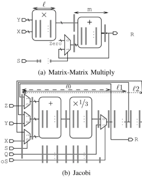
1) Matrix-matrix multiplication: The original code is given in Figure 2(a). The iteration domain is the set integral points lying into a cube of size N, as shown in Figure 2(b). Each point of the iteration domain represents an execution of the assignment S with the corresponding values for the loop counters i, j and k. Essentially, the computation boils down to apply sequentially a multiply and accumulate operation (x, y, z) 7→ x + y ∗ z that we want to compute with a specialized FloPoCo operator (Fig. 4(a)). It consists of a pipelined multiplier with ℓ pipeline stages that multiplies the elements of matrices a and b. In order to eliminate the step initializing c, the constant value is propagated inside loop k. In other words, for k= 0 the multiplication result is added with a constant value 0 (the delayed control signal S is 0). The same

1 typedef float fl ; 2 void mmm(fl∗ a, fl∗ b, fl ∗ c, int N) { 3 int i , j , k; 4 for ( i = 0; j < N; j++) 5 for ( j = 0; i < N; i++){ 6 for (k = 0; k < N; k++) 7 c[ i ][ j ] = c[ i ][ j ] + a[ i ][ k]∗b[k][ j ]; // S 8 } 9 } (a) pipeline size (m) step 0 step 1 step 2 step N-1 H2 ~τ H1 N-1 N-1 tile band ... 0 _J I j tile slice k i (b)

Fig. 2. Matrix-matrix multiplication: (a) C code, (b) iteration domain with tiling

multiplication result is accumulated via the feedback loop in the proper element of the c matrix (when the delayed select line is 1). This result is ready to be reused via the feedback line m cycles later (m is the adder pipeline depth).

There is a unique data dependency carried by the loop k, which can be expressed as a vector ~d= (0, 0, 1) (Fig. 2(b)). The sequential execution of the original code would not exploit at all the pipeline, and will cause a stall of m-1 cycles for each iteration of the loop k due to operator pipelining (ex. between (0, 0, 0) and (0, 0, 1)).

Now, let us consider the affine hyperplane H~τ with ~τ = (0, 0, 1), which satisfies the data dependency ~d and describes a parallel execution front. Each integral point on this hyperplane could be executed in parallel, independently, so it is possible to insert in the arithmetic operator pipeline one computa-tion every cycle. For instance, at iteracomputa-tion (i=0,j=0,k=0): x = c[0][0]=0, y = a[0][0], z = b[0][0]. Then, at iteration (i=0,j=1,k=0): x = c[0][1]=0, y = a[0][0], z = b[0][1]. In this case, the data reuse distance will be N-1, which is normally much larger than the pipeline latency m of the adder, and therefore requiring storing temporally between reuse. To avoid this, we have to transform the program in such a way that: between the definition of a variable at iteration ~i and its use at iteration ~i+ ~d there are exactly m cycles, i.e. ∆( ~d) = m.

The method consists on applying tiling techniques to reduce data reuse distance (Fig. 2(b)). First, as previously presented, we find a parallel hyperplane H~τ (here ~τ = (0, 0, 1)). Then, we complete it into a valid tiling by choosing hyperplanes H1 and H2 (here, the normal vectors are (1, 0, 0) and (0, 1, 0)), H = (H1, H2, H~τ). The final tiled loop nest will have the six nested loops: three inter-tile loops I, J, K iterating over the tiles, and three intra-tile loops ii, jj, kk iterating into the current tile of coordinate (I,J,K).

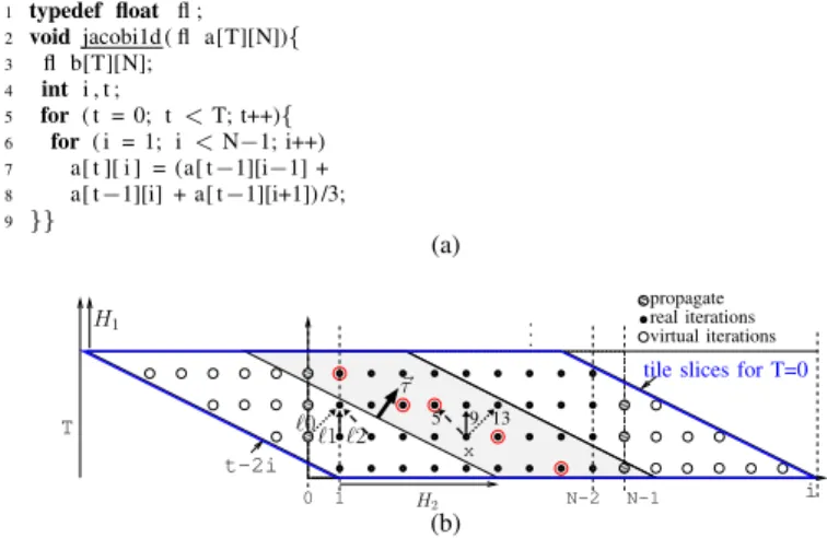
1 typedef float fl ; 2 void jacobi1d ( fl a[T][N]){ 3 fl b[T][N]; 4 int i , t ; 5 for ( t = 0; t < T; t++){ 6 for ( i = 1; i < N−1; i++) 7 a[ t ][ i ] = (a[ t−1][i−1] + 8 a[ t−1][i] + a[ t−1][i+1]) /3; 9 }} (a) 0 .. . 5 9 13 ~τ virtual iterations real iterations propagate t-2i 1 x ℓ1 i T ℓ0 _ℓ2

tile slices for T=0

N-1 N-2 H2

H1

(b)

Fig. 3. Jacobi 1D computation: (a) source code, (b) domain with tiling

For each value of the outermost loop counters (I,J,K,ii), the loops on jj and kk iterate into a tile slice. Figure 2(b) depicts the tile slice for (I=0,J=0,K=0,ii=0). We schedule each tile slice to execute consecutive iterations on the parallel front. Therefore, the main iteration vector can be expressed as (I,J,K,ii,kk,jj).

We select the width of the tile size to be equal to pipeline size m. This ensures that the result produced by the adder is required immediately at its input. Thus, it can be fed imme-diately without any temporary buffering using the feedback connection. The execution order presented above permits to obtain a circuit that computes a temporary value of c each cycle and stores the temporary data inside the pipeline registers of the arithmetic operators, without any temporary storage buffer.

2) Jacobi 1D: The kernel is given in Figure 3(a)). This is a standard stencil computation with two nested loops. This ex-ample is more complex because the set of dependence vectors D contain several dependencies D = { ~d1 = (−1, 1), ~d2 = (0, 1), ~d3 = (1, 1)} (Fig. 3(b)). We apply the same tiling method as in previous example. First, we chose a valid parallel hyperplane. With the normal vector ~τ = (2, 1), H~τ satisfies all the data dependencies ofD. Then, we complete H~τ with a valid tiling hyperplane H1. Here, H1 can be chosen with the normal vector(1, 0). By analogy with the matrix multiply example, we write (T,I,ii,tt) the iteration domain of the result-ing tiled loops. Figure 3(b) shows the consecutive tile slices with T=0. The resulting schedule is valid because it respects the data dependencies of D. The data produced at iteration x must be available 5 iterations later via the dependence ~d1, 9 iterations later via dependency ~d2 and 13 iterations later

via the dependence ~d3. Notice that the dependence distances are the same for any point of the iteration domain, as the dependencies are uniform. In hardware, this translate to add delay shift registers at the operator output and connect this output to the operator input via feedback lines, after data dependency distances levels ℓ0, ℓ1 and ℓ2 (see Fig. 3(b)). Once again, the intermediate value are kept in the pipeline, no additional storage is needed on a slice.

.. . × Y X ℓ Zero R .. . 0 1 .. . S m +

(a) Matrix-Matrix Multiply

0 0 0 1 1 1 Z Y X S .. . + .. . 1 0 .. . .. . Q oS .. . .. . R ×1_/3 ℓ1 _ℓ2 ℓ0 (b) Jacobi

Fig. 4. Computational kernels generated using FloPoCo

As the tiling hyperplanes are not parallel to the original axis, some tiles in the borders are not full parallelograms (see left and right triangle from Fig. 3(b)). Inside these tiles, the dependence vectors are not longer constant. To overcome this issue, we extend the iteration domain with virtual iteration points where the pipelined operator will compute dummy data. This data is discarded at the border between the real and extended iteration domains (propagate iterations, when i= 0 and i = N − 1). For the border cases, the correctly delayed data is fed via line Q (oS=1).

The two next sections formalize the ideas presented in-tuitively on motivating examples and presents an algorithm in two steps to translate a loop kernel written in C into an hardware accelerator using pipelined operators efficiently. Section IV-C explains how to get the tiling. Then, section IV-D explains how to generate the control FSM respecting the schedule induced by the loop tiling.

C. Step 1: Scheduling the Kernel

The key idea is to tile the program in such a way that the distance associated to each dependence is constant. Then, it would be always possible to reproduce the solution described for the Jacobi 1D example.

The only issue is to ensure that the minimum dependence distance is equal to the pipeline depth of the FloPoCo operator. The idea presented on the motivating examples is to force the last intra-tile inner loop Lpar to be parallel. This way, for a fixed value of the outer loop counters, there will be no dependence among iterations of Lpar. The dependencies will all be carried by the outer-loop, and then, the dependence distances will be fully customizable by playing with the tile size associated to the loop enclosing immediately Lpar, Lit.

This amounts to find a parallel hyperplane H~τ (step a), and to complete with others hyperplanes forming a valid tiling (step b): H1, . . . , Hn−1, assuming the depth of the loop kernel is n. Now, it is easy to see that the hyperplane H~τ

should be the (n-1)-th hyperplane (implemented by Lit), any hyperplane Hi being the last one (implemented by Lpar). Roughly speaking, Lit pushes H~τ, and Lpar traverses the current 1D section of H~τ.

It remains in step c to compute the actual dependence distances as an affine function of tile sizes. Then, it is possible to compute the tile size, given a fixed FloPoCo operator pipeline depth. If several dependencies exist, the minimum dependence distance gives the pipeline depth of the operators, and the other distances gives the number of extra shift registers to be added to the operator to keep the results within the operator pipeline, as seen with the Jacobi 1D example. These three steps are described thereafter.

Step a. Find a parallel hyperplane H~τ

This can be done with a simple integer linear pro-gram (ILP). Here are the constraints:

• ~τ must satisfy every dependence: ~τ· ~d > 0 for each dependence vector ~d∈ D.

• ~τ must reduce the dependence distances. Notice that the dependence distance is in-creasing with the radius between the or-thogonal of ~τ , ~τ⊥ and a dependence dis-tance ~d. Notice that the radius (~τ⊥_{, ~d) is} increasing with the determinant det(~τ⊥_{, ~d).} Thus, it is sufficient to minimize the quantity q= max(det(~τ⊥_{, ~d}

1), . . . , det(~τ⊥, ~dp)). So, we build the constraints q ≥ det(~τ⊥_{, ~d}

k) for each k between 1 and p, which is equivalent to q≥ max(det(~τ⊥_{, ~d}

1), . . . , det(~τ⊥, ~d_p)). It remains to find the objective function. We want to minimize q. Then, for the minimal value of q, we want to minimize the coordinates of ~τ . This amounts to look for the lexicographic minima of the

vector (q, ~τ). This can be done with standard ILP techniques [19]. On the Jacobi1D example, this gives the following ILP, with ~τ= (x, y):

min≪ (q, x, y)

s.t. y− x > 0 ∧ y > 0 ∧ y > 0 ∧ x + y > 0 q≥ x − y ∧ q ≥ x + y ∧ q ≥ x

Step b. Find the remaining tiling hyperplanes

Let us assume a nesting depth of n, and let us assume that p < n tiling hyperplanes H~τ, H_φ~

1, . . . , Hφ~p−1 were already found. We can com-pute a vector ~u orthogonal to the vector space spanned by ~τ , ~φ1, . . . , ~φp−1using the internal inverse method [11]. Then, the new tiling hyperplane vector ~

φpcan be built by means of ILP techniques with the following constraints.

• φ~p must be a valid tiling hyperplane: ~φp. ~d≥ 0 for every dependence vector ~d∈ D.

• φ~p must be linearly independent to the other hyperplanes: ~φp.~u6= 0. Formally, the two cases ~

φp.~u >0 and ~φp.~u <0 should be investigated. As we just expect the remaining hyperplanes to

be valid, without any optimality criteria, we can restrict to the case ~φp.~u >0 to get a single ILP. Any solution of this ILP gives a valid tiling hyper-plane. Starting from H~τ, and applying repeatedly the process, we get valid loop tiling hyperplanes H = (H_φ~

1, . . . , Hφ~n−2, H~τ, Hφ~n−1) and the corre-sponding tiling matrix UH. It is possible to add an objective function to reduce the amount of communi-cation between tiles. Many approaches give a partial solution to this problem in the context of automatic parallelization and high performance computing [11], [21], [24]. However how to adapt them in our context is not straightforward and is left for future work. Step c. Compute the dependence distances

Given a dependence vector ~d and an iteration ~x in a tile slice the set of iterations ~i executed between ~x and ~x+ ~d is exactly:

D(~x, ~d) = {~i | UH~x≪ UH~i ≪ UH(x + ~d)} Remember that UH, the tiling matrix computed in the previous step, is also the intra-tile schedule matrix. By construction, D(~x, ~d) is an integral polyhedron (conjunction of affine constraints). Then, the depen-dence distance∆( ~d) is exactly the number of integral points in D(~x, ~d) (that does not depend on ~x). The number of integral points in a polyhedron can be computed with the Ehrhart polynomial method [13] which is implemented in the polyhedral library [6]. Here, the result is a degree 1 polynomial in the tile size ℓn−2 associated to the hyperplane Hn−2, ∆( ~d) = αℓn−2+β. Then, given a fixed input pipeline depth δ for the FloPoCo operator, two cases can arise:

• Either we just have one dependence, D = {~d}. Then, solve ∆( ~d) = δ to obtain the right tile size ℓn−2.

• Either we have several dependencies, D = {~d1, . . . , ~dp}. Then, choose the dependence vec-tors with smallest α, and among them choose a dependence vector ~dm with a smallest β. Solve ∆( ~dm) = δ to obtain the right tile size ℓn−2. Replacing ℓn−2 by its actual value gives the remaining dependence distances ∆( ~di) for i6= m, that can be sorted by increasing order and used to add additional registers to the FloPoCo operator in the way described for the Jacobi 1D example (see figure 4(b)).

D. Step 2: Generating the Control FSM

This section explains how to generate the FSM that will con-trol the pipelined operator according to the schedule computed in the previous section. A direct hardware generation of loops, which is usually used, would produce multiple synchronized Finite State Machines (FSMs), each FSM having an initializa-tion time (initialize the counters) resulting in an operator stall

on every iteration of the outer loops. We avoid this problem by using the Boulet-Feautrier algorithm [12] to generate a single loop that executes one instruction per iterations. The method takes as input the tiled iteration domain and the scheduling matrix (UH) and uses ILP techniques to generate two functions: First and Next. The operations returned by First represents the first operation to be executed. Then, the Next function compute the next operation to be executed given the current operation. The generated code looks like: 1 I := First () ;

2 while(I 6= ⊥) { 3 Execute(I); 4 I := Next(I); 5 }

where Execute(I) is a macro in charge of sending the correct control signals to compute the iteration I of the tile loop. The functions First and Next are directly translated into VHDL if conditions. When these conditions are satisfied, the corresponding iterators are updated and the control signals are set.

The signal assignments in the FSM do not take into ac-count the pipeline level at which the signals are connected. Therefore, we use additional registers to delay every control signal with respect to its pipeline depth. This ensures a correct execution without increasing the complexity of the state machine.

V. REALITYCHECK

Table I presents synthesis results for both our running examples, using a large range of precisions, and two different FPGAs. The results presented confirm that precision selection plays an important role in determining the maximum number of operators to be packed on one FPGA. As it can be remarked from the table, our automation approach is both flexible (several precisions) and portable (Virtex5 and StratixIII), while preserving good frequency characteristics.

The generated kernel performance for one computing kernel is: 0.4 GFLOPs for MMM, and 0.56 GFLOPs for Jacobi, for a 200 MHz clock frequency. Thanks to the efficient FSM generated, the pipelined kernels are used with very high efficiency, more than99% for matrix-multiply, and more than 94% for Jacobi.

Taking into account the kernel size and operating frequen-cies we can clearly claim that we may pack tens, even hun-dreds per FPGA, resulting in significant potential speedups.

VI. CONCLUSION ANDFUTUREWORK

In this paper, we have presented a novel approach using state of the art code transformation techniques to restructure the pro-gram in order to use more efficiently pipelined operators. Our HLS flow starts been implemented in the research compiler Bee, using FloPoCo to generate specialized pipelined floating point arithmetic operators. We have applied our method on two DSP kernels. The obtained circuits have a very high pipelined operator utilization, high operating frequencies, even

TABLE I

SYNTHESIS RESULTS FOR THE FULL(INCLUDINGFSM) MMMANDJACOBI1DCODES. RESULTS OBTAINED USING USINGXILINXISE 11.5FOR

VIRTEX5,ANDQUARTUS9.0FORSTRATIXIII

Application FPGA Precision Latency Frequency Resources (wE, wF) (cycles) (MHz) REG (A)LUT DSPs

Matrix-Matrix Virtex5(-3) (5,10) 11 277 320 526 1 Multiply (8,23) 15 281 592 864 2 (10,40) 14 175 978 2098 4 N=128 (11,52) 15 150 1315 2122 8 (15,64) 15 189 1634 4036 8 StratixIII (5,10) 12 276 399 549 2 (9,36) 12 218 978 2098 4 Jacobi1D Virtex5(-3) (5,10) 98 255 770 1013 stencil (8,23) 98 250 1559 1833 N=1024 (15,64) 98 147 3669 4558 StratixIII (5,10) 98 284 1141 1058 (9,36) 98 261 2883 2266 (15,64) 98 199 4921 3978

for algorithms with tricky data dependencies and operating on high precision floating point numbers.

It would be interesting to extend our technique to non-perfect loop nests. This would require more general tiling techniques as those described in [11]. As for many other HLS tools, the HLS flow described in this paper focuses only on optimizing the performances of the computational part. However, as experience shows, the performance is often bounded by the availability of data. In future work we plan to focus on local memory usage optimizations by minimizing the communication betweeen the tiles. This can be obtained by chosing a tile orientation to minimize the number of de-pendencies that crosses the hyperplane. This problem has been partially solved in the context of HPC [21], [11]. However, it is unclear how to apply it in our context. Also, we would like to focus on global memory usage optimizations by adapting the work presented in [23] to optimize communications with the outside world in a complete system design. Finally, we would like to extend the schedule to apply several pipelined operators in parallel.

REFERENCES

[1] Forte design system: Cynthesizer. http://www.forteds.com [2] Impulse-C, http://www.impulseaccelerated.com

[3] ISE 11.4 CORE Generator IP, http://www.xilinx.com [4] MegaWizard Plug-In Manager, http://www.altera.com [5] Mentor CatapultC high-level synthesis. http://www.mentor.com [6] Polylib – A library of polyhedral functions. http://www.irisa.fr/polylib [7] Synopsys: Synphony. http://www.synopsys.com/

[8] Alias, C., Baray, F., Darte, A.: Bee+cl@k: An implementation of lattice-based memory reuse in the source-to-source translator ROSE. In: International ACM Conference on Languages, Compilers, and Tools for Embedded Systems (LCTES’07) (Jun 2007)

[9] AutoESL: Autopilot datasheet (2009)

[10] Bastoul, C., Cohen, A., Girbal, S., Sharma, S., Temam, O.: Putting polyhedral loop transformations to work. In: LCPC 2003

[11] Bondhugula, U., Hartono, A., Ramanujam, J., Sadayappan, P.: A practical automatic polyhedral parallelizer and locality optimizer. In: ACM International Conference on Programming Languages Design and Implementation (PLDI’08). pp. 101–113. Tucson, Arizona (Jun 2008) [12] Boulet, P., Feautrier, P.: Scanning polyhedra without Do-loops. In: IEEE

International Conference on Parallel Architectures and Compilation Techniques (PACT’98). pp. 4–9 (1998)

[13] Clauss, P.: Counting solutions to linear and nonlinear constraints through Ehrhart polynomials: Applications to analyze and transform scientific programs. In: International Conference on Supercomputing (ICS’96). pp. 278–285. ACM (1996)

[14] de Dinechin, F.: A flexible floating-point logarithm for reconfigurable computers. Lip research report rr2010-22, ENS-Lyon (2010), http:// prunel.ccsd.cnrs.fr/ensl-00506122/

[15] de Dinechin, F., Joldes, M., Pasca, B., Revy, G.: Multiplicative square root algorithms for FPGAs. In: Field Programmable Logic and Appli-cations. IEEE (Aug 2010)

[16] de Dinechin, F., Klein, C., Pasca, B.: Generating high-performance custom floating-point pipelines. In: Field Programmable Logic and Applications. IEEE (Aug 2009)

[17] de Dinechin, F., Pasca, B.: Floating-point exponential functions for DSP-enabled FPGAs. In: Field Programmable Technologies (2010), http:// prunel.ccsd.cnrs.fr/ensl-00506125/

[18] de Dinechin, F., Pasca, B., Cret¸, O., Tudoran, R.: An FPGA-specific approach to floating-point accumulation and sum-of-products. In: Field-Programmable Technologies. pp. 33–40. IEEE (2008)

[19] Feautrier, P.: Parametric integer programming. RAIRO Recherche Op´erationnelle 22(3), 243–268 (1988)

[20] Gupta, S., Dutt, N., Gupta, R., Nicolau, A.: Spark: A high-level synthesis framework for applying parallelizing compiler transformations. International Conference on VLSI Design pp. 461–466 (2003) [21] Lim, A.W., Lam, M.S.: Maximizing parallelism and minimizing

syn-chronization with affine transforms. In: 24th Annual ACM SIGPLAN-SIGACT Symposium on Principles of Programming Languages (PoPL’97). ACM Press (Jan 1997)

[22] Martin, E., Sentieys, O., Dubois, H., Philippe, J.L.: Gaut: An ar-chitectural synthesis tool for dedicated signal processors. In: Design Automation Conference with EURO-VHDL’93 (EURO-DAC’93). pp. 14–19 (Sep 1993)

[23] Plesco, A.: Program Transformations and Memory Architecture Opti-mizations for High-Level Synthesis of Hardware Accelerators. Ph.D. thesis, ´Ecole Normale Sup´erieure de Lyon (2010)

[24] Xue, J.: Loop Tiling for Parallelism. Kluwer Academic Publishers (2000)