HAL Id: hal-01823637
https://hal-amu.archives-ouvertes.fr/hal-01823637
Submitted on 26 Jun 2018
HAL is a multi-disciplinary open access
archive for the deposit and dissemination of
sci-entific research documents, whether they are
pub-lished or not. The documents may come from
teaching and research institutions in France or
abroad, or from public or private research centers.
L’archive ouverte pluridisciplinaire HAL, est
destinée au dépôt et à la diffusion de documents
scientifiques de niveau recherche, publiés ou non,
émanant des établissements d’enseignement et de
recherche français ou étrangers, des laboratoires
publics ou privés.
Subspace SNR Maximization: The Constrained
Stochastic Matched Filter
Bruno Borloz, Bernard Xerri
To cite this version:
Bruno Borloz, Bernard Xerri. Subspace SNR Maximization: The Constrained Stochastic Matched
Filter. IEEE Transactions on Signal Processing, Institute of Electrical and Electronics Engineers,
2011, 59 (4), pp.1346 - 1355. �10.1109/TSP.2010.2102755�. �hal-01823637�
I INTRODUCTION 1
Subspace SNR maximization: the constrained
stochastic matched filter
Bruno Borloz
1,2- Bernard Xerri
1,21
Universit´e du Sud Toulon Var, IM2NP, Equipe ”Signaux et Syst`emes”
2CNRS, IM2NP (UMR 6242)
Bˆatiment X, BP 132, F-83957 La Garde Cedex (FRANCE)
Tel: 33 494 142 461 / 33 494 142 565
Fax: 33 494 142 598
[email protected], [email protected]
Abstract
In this paper, we propose a novel approach to perform detection of stochastic signals embedded in an additive ran-dom noise. Both signal and noise are considered to be real-izations of zero mean random processes whose only second-order statistics are known (their covariance matrices).
The method proposed, called Constrained Stochastic
Matched Filter (CSMF), is an extension of the Stochastic Matched Filter itself derived from the Matched Filter. The
CSMF is optimal in the sense that it maximizes the
Signal-to-Noise Ratio in a subspace whose dimension is fixed a priori.
In this paper, after giving the reasons of our approach, we show that there is neither obvious nor analytic solution to the problem expressed. Then an algorithm, which is proved to converge, is proposed to obtain the optimal solution.
The evaluation of the performance is completed through estimation of Receiver Operating Characteristic curves. Experiments on real signals show the improvement brought by this method and thus its significance.
Keywords— detection ; subspace method ; reduced-rank
method; signal-to-noise ratio maximization; matched filter ; matched subspace.
I. Introduction
This paper deals with the problem of detecting a stochas-tic signal (like a transient signal for example) embedded in an additive random noise.
Throughout this paper, all the signals will be real and discrete (time samples, pixels of images, ...) and repre-sented with vectors of RN.
The method proposed here consists in a linear filtering called (for reasons explained later) ”Constrained Stochastic
Matched Filter” (CSMF). This method gives, for an integer
value p (1 ≤ p < N ), among all the p-dimension subspaces, the one where the Signal-to-Noise Ratio (SNR) is maxi-mum: the CSMF is optimal for this criterion. This is a reduced-rank method (a projection) under constraint (the constraint being the a priori knowledge of the dimension
p) [1].
The SNR is invariant in a p-dimension subspace: it does not depend on the basis chosen to describe the subspace. An important consequence of this invariance of the SNR
w.r.t. the basis is that the simplest basis, say an orthonor-mal one, can usefully be chosen: moreover in such a basis the mathematical expression of the SNR is simple to obtain and will simplify later calculations.
In this paper we show that there is neither immediate nor obvious way to find the optimal p-dimension subspace: then we propose an algorithm and its the convergence to the good solution is proved.
The performances of the method and the comparisons with other methods are performed through the
Receiver-Operating-Characteristic (ROC) curves giving the Proba-bility of Detection PDw.r.t. the Probability of False Alarm
PF A. Nevertheless, this paper gives no demonstration that ROC curves are better for a predicted value of p: we only observe, with results obtained from numerical simulations, that there exists a value of p for which the ROC curve is the best one.
Let us also note that our model is not a parametric one. The only knowledge is the covariance matrices of the ran-dom signals .
A. Problem Formulation
Let us consider an observation x ∈ RN. Two hypotheses can be formally stated (detection problem): this measure-ment was produced by ambient noise n alone or by a signal s embedded in this noise, respectively:
H0: x = n
H1: x = s + n
The objective is to decide between these hypotheses. Our model will not be a parametric one.
The assumptions of our model are the following :
1) s and n are realizations of zero mean ran-dom processes.
2) The covariance matrices of s and n, respec-tively A and B, are supposed to be known, full rank and different.
3) s and n are uncorrelated, not necessarily Gaussian, and their Probability Density Functions (PDF) are unknown.
Two kinds of error are possible: the missing of the signal and the false alarm. A trade-off (highlighted by the ROC curves) must be found between a small average number of misses and a small average number of false alarms.
II OVERVIEW OF SOME EXISTING METHODS
When the PDF of the signals are known, the key quan-tity to compute is the Likelihood Ratio (LR) L(x) which must be compared to a threshold determined according to a criterion such as the minimization of the probability of error, the maximization of PD when PF A is fixed a priori (Neyman-Pearson criterion) [2]-[5].
When the PDF are unknown, L(x) cannot be calculated. This is why we take into consideration methods based on SNR maximization. Furthermore the CSMF method takes place among numerous currently known reduced-rank tech-niques which have been proposed (Section II is a survey of some SNR maximization and reduced-rank methods justi-fying the approach of our method).
B. Why the CSMF ?
When the PDFs are known (e.g. Gaussian), the
Likeli-hood Ratio Test (LRT) is an optimal test which leads to
compare a value to a threshold. For Gaussian signals, the test can easily be written as a sum of N terms (then onto the whole space of the used signals) depending on the ob-servation vector x: log L(x) = Λ(x) = N X i=1 λi 1 + λi(u t ix)2. (1) where the λi (λ1 ≥ λ2 ≥ ... ≥ λN) and ui are respec-tively the eigenvalues and corresponding eigenvectors of B−1A (see Section II-C). In fact, the eigen-elements of B−1A naturally appear when trying to maximize the out-put SNR of a linear filter h: this outout-put SNR can be written
ρ = htAh
htBh.
The maximal value of ρ, noted ρmax, is obtained for h = u1the eigenvector associated with the largest eigenvalue λ1
of B−1A: this filtering consists in a projection of the signal x onto Eu1, and then it is easy to verify that ρmax = λ1. This method is called ”Stochastic Matched Filter” (SMF) [6].
When signals are not Gaussian, we can continue to use Λ(x) which is no longer the log of the LR. This expres-sion has no reason to be optimal, and experimental results show, first, that a truncation of this sum to p terms can improve the ROC curves and next that there exists an op-timal value of p for which the ROC curve is the best one. This truncation (p < N ) is expressed as follows
p X i=1 λi 1 + λi(u t ix)2,
and can be seen as a projection of x onto a p-dimension subspace E†
p: Ep† is spanned by {ui}i=1,...,p. This method, called ”Extended Stochastic Matched Filter” (ESMF) could be wrongly interpreted as a SNR maximization method: in fact it does not maximize the SNR in a p-dimension subspace but a weighted sum of output SNRs, each of them after a projection onto Eui for i = 1, ..., p (see Section II-C).
The method proposed in this paper is naturally inferred from these remarks concerning the output SNR maximiza-tion and the projecmaximiza-tion onto a subspace of dimension two
or higher; therefore its aim is to maximize the SNR in an aptly chosen subspace with an a priori given dimension
p. The choice of p, and then the dimension of the
opti-mal subspace searched for, is a constraint: this is why the name of ”Constrained Stochastic Matched Filter” (CSMF) was given to this optimal filter. We will clearly see that the CSMF is not a simple extension of the ESMF and that the CSMF can no more be inferred from the ESMF.
However, when p = 1, the CSMF and the SMF are iden-tical. But when p > 1, it is proved in this paper (cf. Section III-F) that the optimal space E∗
p cannot be simply deduced from the knowledge of either E†
p or Ep−1∗ . Hence, it is nec-essary to propose an algorithm that finds the solution: this algorithm is given and is proved to converge to the solution (cf. Section IV).
Organization of the paper
In Section I we formulate the mathematical model, present the basic assumptions. Section II describes exist-ing methods and introduces those proposed in the paper. The method is detailed in Section III and useful properties are highlighted. Section IV is dedicated to the practical determination of this subspace: an algorithm is proposed to find the optimal subspace E∗
p and the proof of its con-vergence is given. Then experimental results are presented in Section V.
In this paper, we apply the method to detection, but it could be obviously used for compression, filtering or esti-mation problems.
II. Overview of some existing methods The model is those given in Section I-A.
A. The Karhunen-Lo`eve Transform
The Karhunen-Lo`eve transform (KLT) is a Principal
Component Analysis used to tackle this model [6]-[8] when
noise is white (B = σ2
nI) or absent; it provides the best ap-proximation, in the sense that it minimizes a mean square
error (MSE) for a stochastic signal under the condition
that its rank is fixed and is used for example for data com-pression or filtering. When noise is white, it determines the p-dimension subspace where the SNR is maximum.
But it does not consider colored noise, and therefore is not optimum even when it is used with a noise suppression filter such as the Wiener filter (which is not a reduced-rank method). The SMF, a Generalized Eigen Decomposition (GED) introduced by Cavassilas-Xerri [6] will be detailed in Section II-C: it performs a two-stage operation (pre-whitening and KLT), but is shown to be not optimal in terms of maximization of the SNR. GED is a major prob-lem in many modern information processing applications (adaptive filtering, blind source separation [7], ...) and fast algorithms to estimate and track the principal generalized eigenvectors have been developed [8].
We will show that the CSMF can be seen like an ex-tension of the KLT and the SMF for the problems we are interested in.
II OVERVIEW OF SOME EXISTING METHODS
Some authors want to find an optimal linear data com-pression method in the presence of noise: the Proportional
KLT (PKLT) applies an oblique projection operator onto
a subspace S (dim(S) = p) along a subspace L (S and L are both unknown) [9]. This operator P naturally maxi-mizes a ratio of powers. Solving this problem without any constraint concerning the rank of P naturally leads to an impossibility.
The first part of their work shows how justifiable it is to take an interest in the maximization of the SNR in a subspace.
The CSMF proposed in this paper solves this problem by adding a constraint, the rank of the subspace to project data onto.
B. Parametric Models
For detection with reduced-rank methods, many authors have worked on a parametric model of the following form: x = Hθ + n =Ppi=1θihi+ n (H is a N × p matrix). The useful signal s = Hθ is a stochastic signal constrained to lie in the signal subspace, the p-dimension subspace spanned by the known modes hi, with mode weights or gains, the entries θiof θ. This model in an extension of those used for the Matched Filter (MF) detector, matched to a signal that is assumed to lie in a 1-dimensional subspace (i.e. H = h1
is the deterministic signal to detect).
It is noteworthy that our model is very different, because the covariance matrix A is full rank and then the signal subspace has dimension N .
When the noise is Gaussian, the output of the MF pro-vides a sufficient statistic for any LRT for detection. The knowledge of s and the second-order statistics of n is nec-essary to derive the corresponding MF. For p > 1 the MF detector is no more efficient and is extended to the Matched
Subspace Detector (MSD) [10]-[17] assuming prior
knowl-edge of B. The MF is also named coherent MSD.
When the gains are unknown, the Generalized Likelihood
Ratio Test [5] takes the form of a ratio of two quadratic
forms of prewhitened observations using orthogonal pro-jections onto suitable subspaces. The statistic obtained has natural invariances (the energy of the subspace signal and the SNR are unchanged).
When B is unknown, it is obtained from training data (Adaptive Subspace Detectors) [13][14].
Numerous papers deal with the MF detector and its ex-tensions: several reasons may imply that signal or/and noise are not exactly known (channel nonlinearities, timing jitter, non-stationarities, model uncertainties ...) [18][19].
Another problem studied (e.g. in digital communications [20]) is those of detecting a transmitted signal when one out of several known signals is transmitted. When the additive noise is white and Gaussian, the optimal detector consists of a bank of MF followed by a detector which chooses as the detected signal the one with the maximal output value. Improvements have been observed in many cases [21].
C. The Stochastic Matched Filter and the Extended SMF
C.1 Introduction
The SMF was first introduced to detect a random sig-nal not supposed to lie in a known subspace: furthermore, the second-order statistics of both s and n are supposed to be known [6]. It can be seen like an extension of the MF (it provides an optimal filter since it maximizes the SNR), but also of the KLT. This problem is a generalized eigenvalue problem using the covariance matrices A and B; the filtering is a projection onto the optimal subspace spanned by the eigenvector of B−1A with maximum eigen-value which is also the eigen-value of the maximum output SNR. The output SNR ρ of a linear filter h can be written like a Rayleigh quotient: ρ = htAh
htBh (if A and B have unit trace,
ρ can be interpreted like a gain on the SNR). This
prob-lem is equivalent to solve the following generalized eigen-value problem: Ah = λBh. The maximal eigen-value ρmax is obtained for h = u1 the eigenvector associated with the
largest eigenvalue λ1 of B−1A; then ρmax = λ1 > 1: this
filtering performs a projection of the signal onto E∗
1 = Eu1. If {λi} and {ui} are the eigenvalues and eigenvectors of B−1A with λ1≥ ... ≥ λN, we easily prove that:
I λi ≥ 0 can be interpreted like a gain on SNR after projection onto Eui.
I {ui} is a non-orthogonal basis of RN perform-ing simultaneous diagonalization of A and B. If U = [u1...uN], an appropriate normalization of the ui gives, with ∆ positive diagonal matrix [22]:
½
UtAU = ∆ UtBU = I
The interpretation of the λi naturally leads to take into account directions of projection that could statistically con-tribute to a better detection, that means growing the di-mension of the subspace to project data onto. Actually, it has been shown [6] that a few other eigenvectors, the dominant one, can statistically contribute to improve ROC curves. To take a decision, we have to propose a function of x and the ui.
When the signals are Gaussian, the calculation of the logarithm of the LR leads easily to equation (1). This expression has no reason to be optimal when the signals are not Gaussian, but, according to the remarks above, this summation is shortened to p terms corresponding to significant eigenvalues and the function chosen is then:
Λ(x; p) = p X i=1 λi 1 + λi(u t ix)2, (2)
which is a weighted sum of (ut
ix)2 the power of the ob-servation x after projection onto each direction ui, each weight being linked to the SNR on this direction. This method, called ”Extended SMF” (ESMF), does not maxi-mize the SNR in a p-dimension subspace, but a weighted sum of output SNRs, each of them after a projection onto
Eui for i = 1, ..., p. We will denote E
†
pthe subspace spanned by {ui}i=1,...,p.
III THE CONSTRAINED STOCHASTIC MATCHED FILTER
C.2 Illustration: a practical example
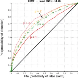
To illustrate the interest of taking into account a sub-space of dimension higher than one, let us apply this method on a narrow-band signal embedded in simulated underwater acoustics: the central frequency is f0 = 3131
Hz and the spectral bandwidth of noise is B = 1260 Hz. The sampling frequency is here Fe = 15423 Hz. Experi-ments are performed on Nr = 1000 realizations of signal denoted si(N = 21, see appendix A) and the initial SNR is about -14 dB. Envelop detection techniques could be used but, in practice, they give lower quality results.
A is calculated as follows: A = NPr i=1
sist
i. For these simu-lations, the areas of presence or not of a signal are obviously known. A detection (which can be a false alarm) is decided each time there are at least 5 consecutive points of the re-sult function done by equation (2) above the threshold.
ROC curves are shown in figure 1, first for p = 1 (E1†) and for the optimal value of p, say 3 (E3†):
0 0.1 0.2 0.3 0.4 0.5 0.6 0.7 0.8 0.9 1 0 0.1 0.2 0.3 0.4 0.5 0.6 0.7 0.8 0.9 1
Pfa (probability of false alarm)
Pd (probability of detection)
ESMF − input SNR = −14 dB
p = 1 p = 2
p = 3 p = 4
Fig. 1. ROC curves (input SNR=−14 dB) for different values of p The improvement brought by projecting data onto E3†
is obvious. This example shows how the make of decision can be greatly improved by taking into consideration more than one eigenvector. Even if the SNR in E3†is smaller than in E1†, we observe that increasing the projection subspace dimension p brings an improvement that is not counterbal-anced by the the decrease of the SNR.
We can also see that there is a worsening of the ROC curve for p = 4. The projection onto E4† will give
statisti-cally worse results than those onto E3†. This result confirms
that there is an optimal value of p for the chosen criterion. C.3 Conclusion
The SMF can be proved to be a two-stage operation: data whitening and then maximisation of SNR in a p-dimensional subspace E†
p (KLT). But, as whitening is not an optimal operation in terms of SNR, the global operation has no reason to maximize the SNR in E†
p. Hence, methods
which try to maximize a SNR while performing a reduced-rank operation are natural when PDF are unknown.
Thus, it seems natural and legitimate to ask oneself if there exists a p-dimensional subspace (p > 1) in which the SNR is maximal, with the hope that ROC curves would be improved again, and then if it is possible to find it. III. The Constrained Stochastic Matched Filter
The method proposed in this paper has been called
Con-strained SMF (CSMF) because it can be seen like an
ex-tension of the SMF, naturally inferred from the remarks in previous section concerning a projection onto a subspace of dimension two or higher where the SNR is maximum.
A. Preliminary remarks and notations
A random signal s, such as in our model, is a vector of RN and can always be expressed as follows:
s = N X i=1
αixi= Xa
where a = [α1...αN]t is a vector of random variables and X = [x1...xN] a basis of RN.
In this paper we are interested only in powers in sub-spaces. Let us denote A = E (sst) the covariance matrix and Ps the power of s. Of course, Ps depends only on the subspace and not on the basis used to describe it, and with no loss of generality, it is possible to consider only or-thonormal bases to describe any subspace: hence XtX = I.
It readily follows that:
Ps= N X i=1 xtiAxi= tr ¡ XtAX¢= tr¡AXXt¢= trA. (3) Moreover, as Ps = trA, we can consider, without loss of generality, only covariance matrices of trace 1.
B. SNR in a p-dimension subspace Ep
Considering an integer p chosen a priori in [1, ..., N − 1], let us denote Ep = E{x1,...,xp} the p-dimension subspace
spanned by the p orthonormal vectors x1 to xp. We
will also denote E⊥
p = E{xp+1,...,xN}. Then, with Xp =
[x1, ..., xp], the projection of s onto Ep along Ep⊥has power
Pp: Pp= tr ¡ Xt pAXp ¢ = p X i=1 xt iAxi, and the expression of the SNR in Ep takes the form:
ρ = p P i=1 xt iAxi p P i=1 xt iBxi = tr ¡ XtpAXp¢ tr¡XtpBXp ¢ . (4)
The objective is to find the unknowns {xi} in order to
maximize this term. The optimal subspace will be denoted
E∗
III THE CONSTRAINED STOCHASTIC MATCHED FILTER
and if covariance matrices A and B have unit trace, ρ is in fact a gain on the SNR (and no longer the output SNR) which can be proved to be necessarily lower than the largest eigenvalue of B−1A, say λ
1[1].
We see here the important difference with the SMF which maximizes the following expression:
ρsmf = p X i=1 vt iAvi vt iBvi ,
where the vi does not form an orthonormal basis.
Throughout the following section, we will focus our at-tention on equation (4) and try to find E∗
p.
C. Characterization of the optimal subspace E∗ p
Let us consider a p-dimension subspace Ep spanned by a set of p orthonormal vectors X = [x1...xp]. The expression
of the SNR ρ in Ep is given by the equation (4).
The constraints can be expressed by the p2relationships
“xt
ixj = δij”. Clearly, p is given and the unknowns of our problem are ρ∗ and the p vectors xi which must be calculated so as to maximize ρ. We are faced with an opti-mization problem with constraints which is usually solved using a Lagrange multipliers method. Let us define the following function: L (X, Ω) = ρ + p X i=1 p X j=1 ωij(xt ixj− δij). (5) This equation can be written:
L (X, Ω) = tr ¡ XtAX¢ tr¡XtBX¢ + tr ¡ Ω¡XtX − I¢¢, (6) where Ω ≡ [ωij] is a p × p symmetric matrix.
A necessary condition for this value to be maximum is ∂L
∂X = 0, which means that for ρ = ρ∗: (A − ρ∗B) X
tr¡XtBX¢ + XΩ = 0.
As B is positive definite, tr¡XtBX¢> 0 and this equation
becomes
(A − ρ∗B) X = XΩ0 (7)
where Ω0is a p×p real symmetric matrix but not diagonal.
But we can find a real orthogonal matrix Π and a real diagonal matrix ∆∗
µ≡ [µ∗i] such that Ω0= Π∆∗µΠt. Then equation (7) becomes:
(A − ρ∗B) XΠ = XΠ∆∗µ. (8) As Π is invertible, XΠ and X span the same subspace
E∗
p. Furthermore, as Π is a real orthogonal matrix, the set of orthonormal vectors X is changed to another set of orthonormal vectors XΠ. Noting XΠ = T∗ = [t∗
1...t∗p], equation (8) can be written
(A − ρ∗B) T∗= T∗∆∗
µ (9)
which is an eigenvalue problem. Note that for any value of
ρ, (A − ρB) is always real symmetric and then
diagonal-izable through a N × N unitary real eigenvector matrix. That means that E∗
p is spanned by a set of p orthonormal vectors which are eigenvectors of (A − ρ∗B). Nevertheless, equation (9) is not simple to solve because, if the t∗
i and
µ∗
i are naturally unknown, ρ∗ is unknown too. For any value ρ > 0 let us denote:
(A − ρB) ti= µiti, i = 1, ...N. (10) (A − ρB) is always real symmetric and the {ti} naturally
form an orthonormal basis.
We note that the eigenvalues µi depend on ρ: it is easy to show, with trivial examples, that they are non nonlinear w.r.t. ρ. A simple illustration is given on figure 2 where we can see the evolution of the eigenvalues µi w.r.t. ρ for the covariance matrices A and B given in example 1 (cf. Section III-F). 0 0.5 1 1.5 2 2.5 3 −1 −0.5 0 0.5 1 evolution of eigenvalues µi w.r.t. ρ ρ µi
Fig. 2. µi(ρ) for example 1 (N = 3)
D. Property of the optimal subspace E∗ p
Equation (10) implies that for any i, j ∈ {1, ...N }, tt
j(A − ρB) ti = µittjti = µiδij. Then for any subset I of {1, 2, ..., N } with cardinality p, X i∈I tt i(A − ρB) ti = X i∈I tt iAti− ρ X i∈I tt iBti= X i∈I µi, so that P i∈IttiAti P i∈IttiBti − ρ = P i∈Iµi P i∈IttiBti . (11)
For the optimal subspace E∗
p, i.e. ρ = ρ∗, the left expression is null, implying that
X i∈I∗
µ∗
i = 0. (12)
This property will be used to find the solution in the two trivial cases ’p = 1’ and ’p = N − 1’ (cf. Section III-E), but also to prove the convergence of the algorithm (cf. Section IV-B).
We have denoted I = I∗; it is easy to show that I∗ =
{1, 2, ..., p} if the eigenvalues are sorted in decreasing order,
say µ∗
1> µ∗2> ... > µ∗N). 5
IV ALGORITHM TO FIND THE OPTIMAL SUBSPACE E∗ P
E. Particular cases
In some particular cases, it is possible to reach the solu-tion easily, without any sophisticated algorithm.
I p = 1
The eigenvalue µ∗
1 to take into account is null. Hence,
(A − ρ∗B) t∗
1 = µ∗1t∗1 = 0, i.e. At1∗ = ρ∗Bt∗1. ρ∗ is the
largest eigenvalue of B−1A and t∗
1 its associated
eigenvec-tor. Naturally we find in this case the SMF. I p = N − 1
AsPN −1i=1 µ∗
i = 0, µN = 1 − ρ∗. Hence, (A − ρ∗B) tN = (1 − ρ∗) tN, or (A − I
N) tN = ρ∗(B − IN) tN; ρ∗ is the largest eigenvalue of (B − IN)−1(A − IN) and tN its asso-ciated eigenvector. The N − 1 vectors spanning E∗
N −1 are the other eigenvectors.
I B = I
In this case, (A − ρI) ti = µiti, i.e. Ati = (ρ + µi)ti. For ρ = ρ∗, Pp
i=1µi = 0 and then Pp
i=1(ρ + µi) = pρ = Pp
i=1λAi (where λAi is the i-th eigenvalue of A), that means
ρ = 1pPpi=1λA
i . Hence the Karhunen-Loeve filter is a par-ticular case of the CSMF.
F. Examples
For the following examples, we state p = 2 and search the optimal subspace E∗
2. As p = N − 1, we can use the
results of the previous paragraph: the SNR ρ∗ obtained in
E∗ 2 is easy to calculate. I Example 1 A =1 3 1.00 0.80 0.640.80 1.00 0.80 0.64 0.80 1.00 , B = 1 3 1.00 0.60 0.360.60 1.00 0.60 0.36 0.60 1.00 .
We denote U and ∆λthe matrices such that AU = BU∆λ: U = 0.6611 −0.70710.3549 0.0000 −0.80760.4170 0.6611 0.7071 0.4170 ,
and λ1 = 1.23, λ2 = 0.56 and λ3 = 0.46. The SNR
obtained in E2† spanned by the eigenvectors associated with the two largest eigenvalues of B−1A (u1 and u2) is
ρ†= 1.06. The SNR obtained in E∗ 2 is ρ∗ = 1.118. If we denote (A − ρ∗B) T∗= T∗∆∗ µ, then: T∗= −0.87910.3370 −0.7071 0.62160.0000 0.4766 0.3370 0.7071 0.6216 , and µ∗ 1 = −0.0725, µ∗2 = −0.1186 and µ∗3 = 0.0725. E2∗ is spanned by t∗
1 and t∗3 (we verify that µ∗1+ µ∗3 = 0 and
µ∗
2= 1 − ρ∗). In this example, since t∗2= u2, E2∗is spanned
by two eigenvectors of B−1A, namely u1and u3which are
clearly not those associated with the two largest λi. I Example 2
Let us consider two covariance matrices of non stationary processes. A = 1 3 0.0379 0.0379 0.15140.0379 0.0473 0.2650 0.1514 0.2650 2.9148 , and B = 1 3 1.2872 1.4658 0.13131.4658 1.6865 0.1629 0.1313 0.1629 0.0263 .
Denote U and ∆λ the matrices satisfying AU = BU∆λ. U = −0.5189 −0.65490.5219 0.7555 −0.39720.9156 0.6770 0.0192 −0.0622 ,
and λ1 = 1051, λ2 = 0.45 and λ3 = 0.01. The SNR
ob-tained in E2† spanned by the eigenvectors associated with the two largest eigenvalues of B−1A is ρ†= 149.64.
The SNR obtained in E∗ 2 is ρ∗ = 151.05. We denote (A − ρ∗B) T∗= T∗∆∗ µ, then: T∗= −0.58450.7111 −0.2531 −0.65590.3057 −0.7516 −0.3908 −0.9179 −0.0695 . and µ∗ 1 = −0.54, µ∗2 = 0.54 and µ∗3 = −150.05. E2∗ is spanned by t∗
1 and t∗2 (we verify that µ∗1+ µ∗2 = 0 and
µ∗
3= 1 − ρ∗). No eigenvector of B−1A is contained in E2∗,
a fortiori the eigenvector associated with the largest
eigen-value of B−1A which generates E∗
1. This example proves
that a recursive algorithm w.r.t. p, that would calculate
E∗
1 and then E2∗, etc... is not realistic.
I Conclusion
From these simple examples, we immediately see that the optimal subspace E∗
p is not necessarily spanned by eigenvectors of B−1A, and even when this is the case, the eigenvectors are not necessarily those associated with the largest eigenvalues. It is not possible to deduce E∗
p from
E†
p. What’s more, it is not possible to find a recursive formulation on p to find E∗
p from Ep−1∗ : for example, the relationship E∗
1 ⊂ E2∗ is not necessarily verified. Then we
have to propose an algorithm to determine E∗
p. This will be performed in Section IV.
G. Conclusion
In this section, the problem has been presented and equa-tions have been deduced that must be solved to find the optimal p-dimension subspace. We have seen that there exists neither analytic nor obvious solution and that an al-gorithm must be proposed. This is the purpose of the next section.
The CSMF consists in finding the p-dimension subspace which maximizes the SNR after only a projection.
IV ALGORITHM TO FIND THE OPTIMAL SUBSPACE E∗ P
IV. Algorithm to find the optimal subspace E∗ p In light of the examples of previous section, it is required to find an algorithm to determine the optimal subspace
E∗
p spanned by p vectors ti verifying equation (10) and maximizing ρ defined by ρ = P i∈IttiAti P i∈IttiBti , (13)
where I is a subset of p different numbers out of {1, ...N }. It seems natural that such an algorithm should be itera-tive and use, at each step, these equations alternately.
A. Presentation of the algorithm
ρ∗ being unknown, it is reasonable to choose for the ini-tial value of ρ, say ρ(0), the largest eigenvalue of B−1A. At each step n ≥ 0, we obtain the symmetric matrix ¡
A − ρ(n)B¢ and calculate its N eigenvectors t(n)
i asso-ciated to eigenvalues µ(n)i . Then we must choose among them the p onesnt(n)i , i ∈ I(n)/card(I(n)) = pofor which
ρ(n+1)= P i∈I(n) t(n)i tAt(n)i P i∈I(n) t(n)i tBt(n)i (14)
is maximum. These p vectors span a subspace Ep(n). Then it is easy to calculate ¡A − ρ(n+1)B¢, I(n+1) and
the new subspace Ep(n+1). This process can be iterated until
|ρ(n+1)−ρ(n)| < ε (see table 1). Of course, we have to prove
that this algorithm converges to the good solution ρ∗.
B. Study of the convergence
At step n, from (11) and (14), the variation of ρ is
ρ(n+1)− ρ(n)= P i∈I(n) µ(n)i P i∈I(n) t(n)i tBt(n)i . (15) Of course, ifPi∈I(n)µ (n) i = 0, then ρ(n+1)= ρ(n). Hence, as it has been proved that for ρ∗, there exists a subset I∗ of cardinal p such as (12) is verified, say Pi∈I∗µ∗i = 0 ,
and ρ∗ is clearly a fixed-point of the algorithm. Let us denote:
X i∈I(n)
µ(n)i = f³ρ(n)´. (16)
Then f (ρ∗) = 0.
As for any value of ρ, A − ρB is symmetrical, the {ti}
span an orthonormal basis: then tt
iti= 1, ∀i. This expres-sion can be differentiated w.r.t. ρ, leading to:
tt i
∂ti
∂ρ = 0, ∀i. (17)
Description of the algorithm ρ(0)= λ1 the largest eigenvalue of B−1A
n = 0
1) Calculate M(n)= A − ρ(n)B
2) Compute the eigenvalues µ(n)i and corresponding eigenvectors t(n)i (i = 1 to N ) of M(n)
(it is possible to sort the eigen-elements so that
µ(n)1 ≥ µ(n)2 ≥ ... ≥ µ(n)N )
3) Find the CNp combinations of p elements out of
{1, 2, ..., N }:
they will be denoted Ik(n)with card³Ik(n)´= p and 1 ≤ k ≤ CNp 4) For k = 1 to CNp Calculate ρ(n+1)k = P i∈I(n)k t(n)i tAt(n)i P i∈I(n)k t(n)i tBt(n)i (k th combination)
5) Find the maximal value of
n ρ(n+1)k o k=1,...Cp N : this maximum is denoted ρ(n+1) 6) If |ρ(n+1)− ρ(n)| < ε stop iterations, t∗ i = t (n) i , µ∗i = µ (n) i , ρ∗= ρ(n+1) Else n ← n + 1, Goto 1) End If E∗
p is spanned by the {t∗i}i∈I∗={1,2,...,p}
Table 1 : description of the algorithm The differentiation of equation (10) w.r.t. ρ leads to
−Bti+ (A − ρB) ∂ti ∂ρ = ∂µi ∂ρ ti+ µi ∂ti ∂ρ.
From equation (17) and multiplying by tt
i, it comes (using equation tt i(A − ρB) = µitti) : −tt iBti+ µitti ∂ti ∂ρ = ∂µi ∂ρ, or ∀i, ∂µi ∂ρ = −t t iBti < 0. (18) Using equations (16) and (18), equation (15) becomes:
ρ(n+1)= ρ(n)+ P i∈I(n) µ(n)i − P i∈I(n) ∂µ(n)i ∂ρ = ρ(n)− f (ρ(n)) f0(ρ(n)), (19)
Obviously f0(ρ∗) is not null: in fact, from (18) we have
f0(ρ) = P i∈I
∂µi
∂ρ < 0 for any value of ρ.
We can use the Newton theorem that says that if :
1) f (ρ) is twice differentiable,
V EXPERIMENTAL RESULTS
2) f (ρ∗) = 0,
3) ρ(0) is “close to” ρ∗,
4) “f0(ρ∗) 6= 0”,
then the series defined by (19) converges to ρ∗ with a quadratic speed. It is easy to prove that I∗ = {1, ...p} (if the eigenvalues are sorted so that µ∗
1 ≥ µ∗2≥ ... ≥ µ∗N)). But we must be careful because that is not true at any step
n for I(n).
Then this algorithm converges to the solution ρ∗ of our problem.
C. Uniqueness of the solution
If we denote λ1 the largest eigenvalue of B−1A, then
1 ≤ ρ∗ ≤ λ
1. In particular cases, it may be possible to
find several subspaces of dimension p for which the SNR ρ is maximal; in fact, this is not a problem. In such a case, we can take an interest in finding a subspace of higher dimension than p with the same SNR, or we can add a new criterion to choose among those subspaces.
D. Practical remark
At each step, the identification of I(n) requires a heavy
calculation. CN
p different combinations have to be tested, which can quickly increase to an unacceptable number of calculations. The algorithm proposed can be improved sig-nificantly. Instead of searching the optimal set of eigen-vectors in a systematic way, one can advantageously re-arrange the eigenvalues of ¡A − ρ(n)B¢ in decreasing
or-der: µ(n)1 > µ(n)2 > ... > µ(n)N (note that those values can as well be positive or negative), and take, at step n,
I(n) = {1, 2, ..., p} (we have seen that I∗ = {1, 2, ..., p}): equation (14) becomes ρ(n+1)= p P i=1 t(n)i tAt(n)i p P i=1 t(n)i tBt(n)i
. In theory, there is no reason for ρ(n+1) to be maximal,
but in practice it so happens that ρ(n+1)reaches almost
sys-tematically the maximal value, and if not, reaches a value very close to it. In the neighbourhood of the solution, the convergence is assured. Such a change of the algorithm ob-viously highly decreases the sum of calculation. In terms of convergence to ρ∗, there is a slight drop in the speed of convergence in terms of number of iterations. Glob-ally, however this method converges to the solution and decreases the sum of calculation in a very significant pro-portion. To give a precise idea of the gain, for N = 21 and
p = 5, CNp = 20349.
The convergence of this modified algorithm has not been proved.
E. Conclusion
In this section, the convergence of the algorithm pro-posed has been proved.
For a given value of p, we have initialized the algorithm with ρ(0) = λ
1 the largest eigenvalue of B−1A, saying it
was reasonable to choose this value. What we are searching for is, p being fixed, the global maximum w.r.t. ρ (there exist other local maxima), and this maximum is necessarily the nearest from ρ = λ1 (1 ≤ ρ∗≤ λ1).
Obviously, an initialization of the algorithm with any value ρ(0)6= λ
1can lead the algorithm to find a local
max-imum.
V. Experimental results
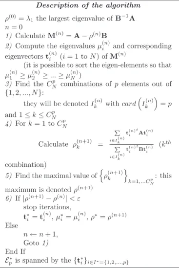
Let us apply the CSMF method to the example described in Section III-F. Results are shown in Figure 3: the quality of the ROC curves increases from p = 1 to p = 4 (or p = 5 which gives more or less the same results than p = 4) and decreases from p = 6. The optimal result is obtained for
p = 4 or 5. 0 0.1 0.2 0.3 0.4 0.5 0.6 0.7 0.8 0.9 1 0 0.1 0.2 0.3 0.4 0.5 0.6 0.7 0.8 0.9 1 CSMF : input SNR = − 14 dB p = 1 p = 2 p = 3 p = 4 p = 5 p = 6 Pd (probability of detection)
Pfa (probability of false alarm)
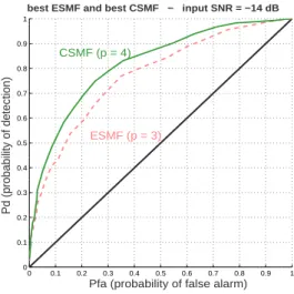
Fig. 3. CSMF : ROC curves for different values of p Figure 4 shows the best result obtained by the CSMF (E∗
4) and the best one obtained by the ESMF (E3†). The
ROC curve obtained in E∗
4 (the best result reachable) is
obviously above those obtained in E3†. Note that E∗
1 = E1†. 0 0.1 0.2 0.3 0.4 0.5 0.6 0.7 0.8 0.9 1 0 0.1 0.2 0.3 0.4 0.5 0.6 0.7 0.8 0.9 1 Pd (probability of detection) Pd (probability of detection)
Pfa (probability of false alarm) bset
best ESMF and best CSMF − input SNR = −14 dB
ESMF (p = 3)
CSMF (p = 4)
Fig. 4. Best ROC curves for CSMF (p = 4) and ESMF (p = 3) This example illustrates clearly the improvement that
VI CONCLUSION
can be brought by maximizing the SNR in E∗
4 instead of
E∗
1, but also its superiority in comparison with the ESMF
method.
Now the optimal subspace E∗
p (here p = 4) has been found with the CSMF method which is a projection (a reduced-rank method). Nevertheless we did not use all the possibilities of classical filtering, and among all the basis of
E∗
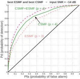
p, we can choose one with interesting properties after a linear filtering. For example, the ESMF gives preferential treatment to directions (spanned by the ui) with the best SNR (λi) (like the Wiener filter): after this linear filtering, the power of noise is one in any direction ui.
Thus, we calculate the ROC curves obtained with the equation (2) where p is the subspace dimension so that all the basis vectors of E∗
4 are taken into account. Results are
shown in figure 5. 0 0.1 0.2 0.3 0.4 0.5 0.6 0.7 0.8 0.9 1 0 0.1 0.2 0.3 0.4 0.5 0.6 0.7 0.8 0.9 1 Pd (probability of detection) Pd (probability of detection)
Pfa (probability of false alarm) bset
best ESMF and best CSMF − input SNR = −14 dB
ESMF (p = 3)
CSMF (p = 4) CSMF+ESMF (p = 4)
Fig. 5. ROC curves for SNR=-14 dB
A noteworthy improvement can be observed by using a simultaneous diagonalization technique in the optimal sub-space calculated beforehand. We finally used a projection (to find the optimal subspace) and a linear filtering opera-tion to improve again the detecopera-tion.
VI. Conclusion
The method proposed in this paper takes its place in the set of methods of decomposition of signals on appropriate basis but also in subspace methods.
When trying to detect stochastic signals with known co-variance matrices but with no a priori knowledge on their probability density function, people usually try to project on the signal subspace (SVD,...). It is possible to take into account the structure (covariance) of the embedding noise: the SMF is used in such a point of view and in this case, a projection onto a p-dimensional subspace is made. In fact, this method is proven to be equivalent to a two-stage method: the whitening of the noise followed by the max-imization of the SNR in a p-dimensional subspace. This method comes down to projecting the observation onto a subspace of dimension greater than one. However, there is no guarantee that the signal-to-noise ratio is maximum in
the subspace spanned by these vectors.
In this paper, we calculate a subspace whose dimension is chosen a priori and which is optimal in the sense that the SNR ratio is maximized within. We prove, through theoretical examples, that this subspace is not necessar-ily those spanned by the vectors calculated by the SMF. Through ROC curves, practical experimentations illustrate the interest of such an approach.
We have shown, with a practical example, that a note-worthy improvement can be reached with the ESMF ap-plied in the optimal subspace calculated beforehand by the CSMF. It confirms that such a method is an interesting and powerful one to perform detection.
Prospects of applications of the CSMF can easily be imagined in image processing or stochastic transient sig-nals detection (like acoustic sigsig-nals). An extension to the classification problem is possible. Of course, as this method is a reduced-rank one performing SNR maximization, it can be used for data compression or estimation and filtering. Thus, the CSMF was successfully used with real signals:
• analysis of sequences of IR images (SATIR) to qual-ify high heat flux components (carbon bricks used in the ITER project with the CEA Cadarache): detection of de-fects and classification of components [23],
• detection and classification of textured images (like expanded polystyrene and textured paper or textured stones pictures for example): lot of images are texture im-ages (forests, farming areas, ...) [1],
• detection and localization of very high energy neutrinos by a passive underwater acoustic telescope (ANTARES European project) [24],
• estimation of the sources in a specific blind source separation problem [25].
Reduced-rank estimators and filters are important for a wide range of signal processing applications, among others when data or model reduction, robustness against noise or model errors is desired. This concerns known methods like the reduced-rank Wiener filter (RRWF) by Scharf [17], the reduced-rank maximum likelihood estimation (RRMLE) by Stoica-Viberg [26], the relative Karhunen-Loeve
trans-form (RKLT) by Yamashita-Ogawa [9] or the generalized Karhunen-Loeve transform (GKLT) by Hua-Liu [27], which
is used for data compression and filtering and is in fact nothing else than the RRWF also called low-rank Wiener
filter in [28] section 8.4.
The choice of the optimal dimension p of the subspace of projection is an important question which must be ex-amined in more detail in the future.
Appendix A : Matlabr code.
I In the main program B = 1260 % (Hz) noise bandwith f0 = 3131 % (Hz) central frequency fe 15324 % (Hz) sampling frequency
Z = reponse(f0,0.25,fe); % generation of a narrow-band signal
signal = create(Ls,Z); % Ls = length of the signal 9
VI CONCLUSION
Z = reponse(f0,B,fe); % generation of the noise noise = create(Ln,Z); % Ls = length of the noise
I subroutine 1 function y = create(lg,filtre) n = length(filtre); X = randn(1,lg+n); X1 = conv(X,filtre); X1 = X1/std(X1); y = X1(n:length(X1)-n); end I subroutine 2 function Z = reponse(F0,B,fe) Te = 1 / fe; n0 = round( 1/(2*B*Te)); n = 1 : (2 * n0 + 1); Z = cos(2*pi*F0*(n-1-n0)*Te).*sin(2*pi*B*(n-1-n0)*Te)./(pi*(n-1-n0)*Te); Z(n0+1) = 2 * B; end
The realizations si(i = 1, ..., Nr) are generated by taking
N consecutive points in the narrow-band signal, the first
point being chosen randomly. References
[1] B. Borloz, Estimation, d´etection et classification par
maximisa-tion du rapport signal-`a-bruit : le filtre adapt´e stochastique sous
contrainte, Ph.D. Thesis, University of Toulon-France, Jun. 2005.
[2] H.L. Van Trees, Detection, Estimation and Modulation Theory,
Radar-Sonar Signal Processing and Gaussian Signals in Noise, Wiley, Part III. 2001
[3] H.V. Poor, An Introduction to Signal Detection and Estimation,
Springer-Verlag, 1988.
[4] T. Kailath, H.V. Poor, Detection of Stochastic Processes, IEEE
Transactions on Information Theory, Vol.44, no.6, pp.2230-2259, Oct. 1998.
[5] A. Hero, Signal Detection and Classification, in ’The Digital
Signal Processing Handbook’ by Vijay K. Madisetti. CRC Press LLC, Series: Electrical Engineering Handbook, 1997.
http://www.eecs.umich.edu/∼hero/Preprints/crc article.ps.Z
[6] J.F. Cavassilas, B.Xerri, Extension de la notion de filtre adapt´e.
Contribution `a la d´etection de signaux courts en pr´esence de
termes perturbateurs, Revue Traitement du Signal vol.10 no.3,
pp.215-221, 1992.
[7] P.P.Pokharel, U. Ozertem, D. Erdogmus and J.C.Principe
Recur-sive complex BSS via generalized eigendecomposition and appli-cation in image rejection for BPSK, Signal Processing, vol.88,
pp.1368-1381, 2008.
[8] J. Yang, H.S. Xi, F. Yang and Y. Zhao RLS-based adaptive
al-gorithms for generalized eigendecomposition, IEEE Trans. Signal
Processing, vol.54, no.4, pp.1177-1188, Apr. 2006.
[9] Y. Yamashita, H. Ogawa, Relative Karhunen-Loeve transform ,
IEEE Trans. Signal Processing, vol.44, pp. 371-378, Feb. 1996.
[10] L.L. Scharf and B. Friedlander: Matched Subspace Detectors
IEEE Trans. Signal Processing, vol.42, no.8, pp. 2146-2157, Aug. 1994.
[11] Mukund N. Desai and Rami S. Mangoubi, Robust Gaussian and
Non-Gaussian Matched Subspace Detection, IEEE Trans. Signal
Processing, vol.51, no.12, pp.3115-3127, Dec. 2003.
[12] Mukund N. Desai and Rami S. Mangoubi, Robust Subspace
Learning and Detection in Laplacian Noise and Interference,
IEEE Trans. Signal Processing, vol.55, no.7, pp.3585-3595, Jul. 2007.
[13] S. Kraut, L.L. Scharf and L. Todd McWhorter Adaptive
Sub-space Detectors IEEE Trans. Signal Processing, vol.49, no.1,
pp.1-16, Jan. 2001.
[14] S. Kraut and L.L. Scharf The CFAR Adaptive Subspace Detector
is a Scale-Invariant GLRT IEEE Trans. Signal Processing, vol.47,
no.9, pp.2538-2541, Sept. 1999.
[15] L.L. Scharf and S. Kraut Geometries invariances, and SNR
in-terpretations of matched and adaptive subspace detectors
Traite-ment du Signal, vol.15, no.6, pp.527-534, 1998.
[16] L.L. Scharf, Shawn Kraut, Michael L. McCloud A Review of
Matched and Adaptive Subspace Detectors Proc. Symp. on
Adap-tive Systems for Signal Process. Commun. and Control, Lake Louise, Alta., Canada, Oct. 2000.
[17] L.L. Scharf and M.L. McCloud Matched and Adaptive Subspace
Detectors When Interference Dominates Noise Proc. Asilomar
’00, Monterey, CA, Oct. 2000 (invited).
[18] S. Verdu, H.V. Poor, Signal Selection for Robust Matched
Filter-ing, IEEE Trans. on Communications, vol.COM-31, no.5,
pp.667-670, May. 1983.
[19] S. Verdu, H.V. Poor, Minimax Robust Discrete-time Matched
Filters IEEE Trans. Communications, vol.COM-31, no.2,
pp.208-215, Feb. 1983.
[20] J.G. Proakis, Digital Communications, McGraw-Hill, Inc., third
edition, 1995.
[21] Y.C. Eldar, A.V. Oppenheim, Orthogonal Matched Filter
De-tection, Proceedings on the International Conference Acoustics,
Speech, Signal Processing (ICASSP-2001) Salt-Lake, UT, May. 2001.
[22] R.A. Horn and C.R. Johnson, Matrix analysis, Cambridge
Uni-versity Press, ISBN 0-521-38632-2, 1999.
[23] F. Cismondi, B. Xerri, C. Jauffret, J. Schlosser, N. Vignal and A.
Durocher Analysis of SATIR Test for the Qualification of High
Heat Flux Components: Defect Detection and Classification by Signal-to-Noise Ratio Maximization Physica Scripta, T. 128, pp
213-217, Mar. 2007.
[24] N. Juennard, C. Jauffret, B. Xerri Detection and Localization of
Very High Energy Neutrinos by a Passive Underwater Acoustic Telescope Passive’08 , IEEE OES , Hy`eres, 14-17, Oct. 2008.
[25] B.Xerri, B.Borloz Detection by SNR maximization: application
to the blind source separation problem, 5th International
Con-ference On Independant Component Analysis and Blind Signal Separation. Sept. 22-24 2004. Grenade (Spain)
[26] P. Stoica and M. Viberg Maximum Likelihood Parameter and
Rank Estimation in Reduced-Rank Multivariate Linear Regres-sions, IEEE Trans. Signal Processing, vol.44, pp. 3069-3078, Dec.
1996.
[27] Y. Hua and W. Liu, Generalized Karhunen-Loeve Transform ,
IEEE Signal Processing Lett., vol.5, pp.141-142, Sept. 1994.
[28] L.L. Scharf Statistical Signal Proces.: Detection, Estimation
and Time Series Analysis Reading MA; Addison Wesley, 1991.
Annex : Notations C ≡ [cij] : matrix of entries cij Ct : transpose of C C−1 : inverse of nonsingular C trC : trace of C I : N × N unity matrix 0 : N × N null matrix
∆λ≡ [λi] : diagonal matrix of entries λi
v : column vector
E[.] : expected value of [.]
δij : Kronecker delta of rank 2
s : signal of interest
n : corrupting noise
A : N × N full-rank covariance matrix of s
B : N × N full-rank covariance matrix of n
λi : eigenvalue of B−1A (with λ1≥ λ2≥ ... ≥ λN≥ 0) ui : eigenvector of B−1A µi : eigenvalue of (A − ρB) ti : eigenvector of (A − ρB) Ep : subspace of dimension p
Ep† : subspace of dimension p spanned by {u1, ..., up}
Eu : subspace of dimension 1 spanned by u
E∗