HAL Id: hal-00776142
https://hal.archives-ouvertes.fr/hal-00776142
Submitted on 15 Jan 2013
HAL is a multi-disciplinary open access
archive for the deposit and dissemination of
sci-entific research documents, whether they are
pub-lished or not. The documents may come from
teaching and research institutions in France or
abroad, or from public or private research centers.
L’archive ouverte pluridisciplinaire HAL, est
destinée au dépôt et à la diffusion de documents
scientifiques de niveau recherche, publiés ou non,
émanant des établissements d’enseignement et de
recherche français ou étrangers, des laboratoires
publics ou privés.
Toward a decompositional and incremental approach to
diagnosis of dynamic systems from timed observations
I. Fakhfakh, M. Le Goc, L. Torres, C. Curt
To cite this version:
I. Fakhfakh, M. Le Goc, L. Torres, C. Curt. Toward a decompositional and incremental approach to
diagnosis of dynamic systems from timed observations. 23rd International Workshop on Principles of
Diagnosis, Great Malvern, Jul 2012, Great Malvern, United Kingdom. 8 p. �hal-00776142�
systems from timed observations
Ismail Fakhfakh
1, Marc Le Goc
2, Lucile Torres
2, and Corinne Curt
11
IRSTEA, 3275 route de C´ezanne - CS 40061, Aix-en-Provence, France [email protected]
2
LSIS, Aix-Marseille Univ, 13397 Marseille, France [email protected]
A
BSTRACTIt is now well-known that the size of the model is the bottleneck when using model-based ap-proaches to diagnose complex systems. To an-swer this problem, decompositional and multi-modeling approaches have been proposed. In this paper, we propose a multi-modeling method called TOM4D (Timed Observations Modeling for Diagnosis) able to cope with dynamic as-pects. It relies on four models: perception, struc-tural, functional and behavior models. The be-havior model is described through system compo-nent models as a set of compocompo-nent behavior mod-els and the global diagnosis is computed from the component diagnoses (also called local diag-noses).
Another problem, which is far less considered, is the size of the diagnosis itself. However, it can also be huge enough, especially when deal-ing with dynamic system. To solve this problem, we propose in this paper to use The Timed Obser-vation Theory.
In this context, we characterize the diagnosis us-ing TOM4D and the timed observation theory. We show their relevance to get a tractable rep-resentation of diagnosis. To illustrate the impact on the diagnosis size, experimental results on a hydraulic example are given.
1 INTRODUCTION
Diagnosis is concerned with the development of algo-rithms and techniques to determine why a correctly de-signed system does not work as expected. The compu-tation is based on observations, which provide infor-mation on the current behavior. The aim of diagnosis is to detect and identify the reason for any unexpected behavior, and to isolate the parts which fail in a system. The systems to be diagnosed can be of different types, like static or dynamic systems, or systems that work with discrete or continuous domains. Moreover, the information of the system, from which the diagno-sis is performed, can be qualitative, logic or quantita-tive. The diagnoser depends essentially on the
man-ner in which (i) the observations are presented (ii) the system is modeled. In fact, in dynamic systems, the observation is timed unlike in static systems where the observations are given at only one point of time. The Timed Observation Theory of Le Goc (Le Goc, 2006) provides a general mathematical framework for mod-eling dynamic processes from timed data. This theory is important because it can be applied to all observed systems. The extension of this framework has given birth to a modeling approach for diagnosis based on timed observation theory called TOM4D. The aim of the modeling approach is to have an efficient diagnosis based on the constructed models.
For complex and large systems, the impossibility of defining a global behavior model makes it necessary to build the behavior model by breaking down and de-scribing the behaviors of each component of the sys-tem. We extend the TOM4D method to cope with de-compositional approach. In this case, diagnoses are computed locally for each component before being merged to obtain a global diagnosis.
In this paper, after a brief presentation of the Timed Observation Theory and the TOM4D method (Sec-tions 2 and 3), we show how TOM4D supports the modeling of complex physical systems. In section 4, we show how the models can be used to characterize the diagnosis. Then, we demonstrate that the diagno-sis can be computed from the TOM4D models. We apply the modeling approach and the diagnosis algo-rithm to an hydraulic system. Section 5 provide an application of our approach to the hydraulic system. Finally, Section 6 provides conclusions and proposes some perspectives of this work.
2 TIMED OBSERVATION THEORY
This theory defines a dynamic system as a process P r(t)={x1(t), x2(t), ..., xn(t)} of timed functions
xi(t) defined on R (i.e. signals provided by sensors).
A timed observation is a couple (δi, t
k) which
corre-sponds to the assignation of a predicate θ(xi, δij, tk)
where δi
jis constant and tk ∈ R a time stamp. When
making an abuse of language, such a predicate can al-ways be interpreted as the predicate EQUALS(xi, δji,
23ndInternational Workshop on Principles of Diagnosis
tk) (i.e. xi(tk) = δji). A monitoring programΘ(X, ∆)
is a programΘ that analyzes the set of time functions xi(t) associated to the set of variables X ={xi}i=1,...,n
. The aim of a monitoring program is to write timed observations (δi, tk) in a database whenever a time
function xi(t) ∈ X(t) satisfies some predicate θ(.. ,..
,..). This leads to define the Observation class as fol-lows:
Definition 1 (An observation class). Let X be a set
of variable names of a processP r(t)={x1(t), x2(t),
...,xn(t)} and let ∆= ∪ xi∈X
∆xibe such that∆xi is a set of values assumable by the variablexi∈ X via a
programΘ. An observation class Ci={(x
i,δji), (xi+1,
δj+1i+1), ..., (xi+n,δj+ni+n} is a set of couple (xi,δij)
as-sociating a variable xi, eventually unknown, with a
constantδi j.
In other words, an observation class Ci associates
variables xi ∈ X with constants δji ∈ ∆xi. For
sim-plicity reasons, an observation class is usually defined as a singleton Ci={(xi, δij)}.
Proposition 2.1. is immediate consequences of
defini-tion 1 : each timed observadefini-tion o(tk)≡ (δji,tk)
corre-sponds to an occurence of an Observation classCi=
{(xi,δji)}.
3 MODELING FRAMEWORK FOR DIAGNOSIS : TOM4D
3.1 General Presentation of TOM4D
TOM4D is a modeling method for dynamic systems focused on timed observations. The objective of this method is to produce a suitable model for dynamic process diagnosis from timed observations and experts a priori knowledge. TOM4D relies on the idea that experts use an implicit model to both formulate the knowledge about the process and diagnose it. It is a multi-model approach that combines CommonKads templates (Schreiber et al., 2000) with the conceptual framework proposed in (Zanni et al., 2006) and the tetrahedron of states (T.o.S), (Rosenberg and Karnopp, 1983), (Chittaro et al., 1993). These elements are merged according to the Timed Observations Theory (Le Goc, 2006).
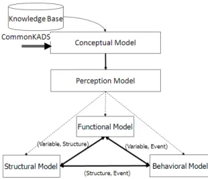
These concepts of component, variable and obser-vation class allow to organize the available knowl-edge about a process P r(t) according to a Struc-tural Model SM(P r(t)) defining the components of the process and their relations, a Functional Model F M(P r(t) defining the values of the process vari-ables (i.e. their definition domain) and the relations between the variables values with a set of mathe-matical functions, and a behavior Model BM(P r(t)) defining the timed observation classes firing the evo-lutions of the time functions of P r(t). A complemen-tary model, the Perception Model P M(P r(t)) of the process, specifies the process variables, the operating goals and the normal and abnormal operating behav-iors (cf. Figure 1). Consequently, a model M(P (t)) of a process is a quadruplet M(P r(t)) = < P M (P r(t)), SM(P r(t)),F M (P r(t)), BM (P r(t)) >.
Figure 1: TOM4D Modeling Process
3.2 Improving representation in a decompositional Approach
Real-world systems can often be seen as a set of inter-connected components. Each component has a simple behavior but the connections between the components can lead to a complex global model. For this reason, the size of a global model of the system is generally in-tractable and no global model can be effectively built. The TOM4D method associates a variable xki with one
and only one component ck. This allow to
decom-pose the dynamic process P r as a set of subprocess P rk representing the different variables of component
system ck. In the following, we give the definitions
of component and the properties the set of component models must satisfy to get a safe representation of the system model.
Definition 2 (system and components). A system can
be described by its set of components COMPS ={c1,
...,cn}. Each component ckis defined as a subprocess
P rk(t)={xk1(t), xk2(t), ..., xkm(t)} of timed functions
xki(t). A system is viewed as a set of sub-process of P r(t) = {P r1(t), ..., P rn(t)}
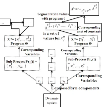
The representation of the Timed Observation The-ory with the decompositional system is summarized in Figure 2.
The idea is to describe the TOM4D approach at two levels namely the components of the system (compo-nent representation) and the system considered as a whole (system representation). The following sections provide a succinct description of the TOM4D approach at two levels (component and global).
3.3 Model of a component
A model of the component ck is a quadruplet
M(P rk(t)) of a process P rk(t) : M(P r(t)) =
< CP M(P rk(t)), CSM (P rk(t)),CF M (P rk(t)),
CBM(P rk(t)) >, where CPM, CSM, CFM, CBM
are respectively component perception model, com-ponent structural model, comcom-ponent functional model and component behavior model.
Figure 2: Timed Observation Theory extend to decom-positional approach
Component Structural Model
The interpretation of the knowledge base with the T.O.S (Tetrahedron of States) allows to define an ab-stract generic representation of the component. The abstract model represent the structural model of the component.
Component Functional Model
The Component Functional Model describes the rela-tions between the values of the variables of the com-ponent ckwith mathematical functions.
Component behavior Model
The component behavior Model BM(P rk(t)) of a
sub-process P rk(t) describes its operating modes with
a set of states and observation classes triggering the state transitions. The behavior model is the key com-ponent of the multimodeling approach, notably be-cause the diagnosis reasoning process is based on this model. The behavior model is defined as follow: Definition 3 (Component behavior Model). Let Xkbe a set of observable variables of a component ck. A
component behavior modelCBM(P rk(t)) of this one
is a 3-tuple< Sk,Ck,γ
k> such that,
• Skis a set of system states defined asSk ={sk:
Xk → ∆xk i as sk(xk i) =δx k i, xk i ∈ Xk,δx k i ∈ ∆xk i },
• Ckis a set of observation classes where an
obser-vation class is a set of discrete events; in partic-ular, an observation class associated with a vari-ablexk i ∈ Xk is a setCx k i = { (xk i, δ) as δ∈ ∆xk i},
• γk: Sk× Ck→ Sk is a function of state
transi-tion.
Figure 3: TOM4D presented in decompositional ap-proach
3.4 Model of a System
The model of a system is M(P r(t)) = < M (P r1(t)),
...,M(P rn(t)), F GM(P r(t)), SGM (P r(t)) >,
where M(P rk(t)) = < CP M(P rk(t)),
CSM(P rk(t)), CF M(P rk(t)), CBM(P rk(t))
> is the Process Model of the component ck,
SGM(P r(t)) is the global structural model and F GM(P r(t)) is the global functional model. The global model M(P r(t)) is built to be a decomposition of the component models M(P rk(t)). The relations
between the different component models M(P rk(t))
is provided by the variables and defined in the Global Functional Model and the Global Structural Model (cf. Figure 3).
Global Structural Model
The Global Structural Model describes relations be-tween the components of the system and the relations between the components and the variables.
Global Functional Model
The Functional Model describes the relations between the values of the variables of different components with mathematical functions.
4 DIAGNOSIS
4.1 Diagnosis characterization
This section provides a characterization of diagnosis in terms of TOM4D method and Timed Observations Theory. The system we consider is decompositional systems composed of n components (represented by n behavior models) which interact each other. We start by characterizing the diagnosis for one compo-nent then we generalize the algorithm for the whole of the system.
Each components behavior model CBM(P rk(t))
is described as a set of states and the possible transi-tions between them. A state transition is triggered by the occurrence of a timed observation : according to the Timed Observations Theory, such an occurrence is recorded when a variable assumes a new value. A state path (S-Path) of the component ck between two states
sk
i and skj is a suite(ski, ski+1, ..., skj) of (j − i + 1)
states linking the initial state sk
i to the final state skj in
23ndInternational Workshop on Principles of Diagnosis
the following definition of a state path in a behavior model:
Definition 4 (S-Path). Let CBM(P rk(t)) = ≺ Sk,
Ck,γk≻ a behavior model of the process P rk(t)
rep-resenting the component ck. A State Path is a suite
Sk
i,j=(ski, ski+1, ..., skj) of (j − i + 1) states linking the
initial statesk
i to the final stateskj.
The observations ω can generally be deccomposed as follows: ω ={ω1, . . . ,ωn} such that ωk contains
the timed observations from the component ck. Local
diagnosis for the component ck is performed starting
from a set of local timed observations ωkand the
com-ponent behavior model CBM(P rk(t)) of the
com-ponent ck defined in TOM4D method. It consists in
explaining the observations sent by the ωk during the
period [t0, tn]. The set of S-Path consistent with the
BM(P rk(t)) represents the possible states occupied
by the component during the period [t0, tn].
Conse-quently, the local diagnosis is represented by a set of S-Path, each S-Path of which represents a possible or-der of states of the component ckin different instances
t∈ [t0, tn].
Definition 5 (Local diagnosis definition). Given the
component Behavior Model CBM(P rk(t)) of the
component ck and the local observations ωk =
{o(t0), ..., o(tn)} contains n + 1 timed observations
from the component ck recorded during the period
[t0, tn] a diagnosis Dck(t) = {S
k
i,j} is the mininal set
of S-PathSi,jk consistent withCBM(P rk(t)) and ωk.
ωk, CBM(P rk(t))) → Dck(t) (1)
These diagnoses represent the component behaviors that are consistent with the local observations. Only the S-Path leading the system to explain all the obser-vations timed are those of interest for our local diag-nosis purpose.
As a consequence, the global diagnosis D(t) is a combination of each local diagnosis Dci(t) at different
instance of diagnosis:
Definition 6 (Global diagnosis definition). Given a set
of n local diagnosis{Dc1, ...,Dck, ...,Dcm } describ-ing the possible states occupied by the different com-ponents ck during the period [t0, tn], noted Sk. A
global diagnosis D for the system is the set of state paths S =S1× .... × Smconsistent with the TOM4D
models.
Dc1(t), ..., Dcm(t), GF M (P r(t)), GSM (P r(t))
→ D(t) In other words, the global diagnosis correspond ex-actly to the Cartesian product of the different possible states of the components at different instance and con-sistent with the global functional and global structural model of the system.
A dynamic system must continuously operate in the face of changing conditions. In the context of diag-nosis, the dynamic system provides continuously new observations for its variables. According to the Timed Observation Theory, a new observation correponds to the appearance of a timed observation. Each timed ob-servation corresponds to an occurence of an Observa-tion class. A change of state is determinated by the
occurrence of an observation class, that is to say when a variable assumes a new value.
As a consequence, the diagnosis D(tk) reasoning
process must be triggered by each timed observation of a suite ω ={o(t0), ...,o(tn)} during the period [t0, tn]
in order to produce the minimal set of possible state paths that are consistent with the timed observations o(tk) ∈ ω. We will propose an incremental
proce-dure to compute a diagnosis for a system description (M(Pr(t)), ω) and its successive new timed observa-tions according to the presented definiobserva-tions.
4.2 Diagnosis Algorithm
The algorithm to compute a diagnosis given a TOM4D model M(P r(t)) and a suite ω = {o(t0), ...,o(tn)} of
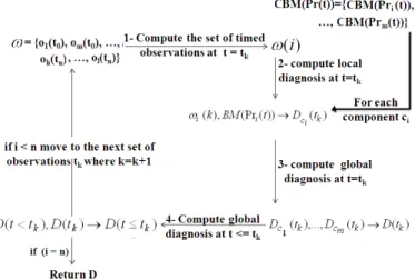
n+ 1 timed observations recorded during the period [t0, tn] is graphically represented in Fig 4.
Figure 4: principle of calculating the global diagnosis of a dynamic system decomposed
Step 1 : Compute the set of timed observations at t= tk
The first step of the algorithm applies the supperpo-sition theorem of the Timed Observation Theory for each time tk ∈ [t0, tn]. This theorem allows to
de-compose the suite ω in a set{ω1, ..., ω2, ..., ωm} of m
suites ωi of (local) timed observations where each ωi
corresponds to the set of the timed observations of a component ci.
Step 2 : Compute Local Diagnosis att= tk
The aim of the second step is to compute the local diagnosis ωi(k), CBM (P ri(t)) → Dci(tk) for each
component ci∈ C at time tk.
Step 3 : Compute Global Diagnosis att= tk
At each time tk, the diagnosis algorithm aims then to
compute each local diagnosis Dci(tk)={S
i
h,m} and to
combine each path sets{Si
h,m} to build a unique path
set D(tk) = Si,jcorresponding to the global diagnosis
D(tk).
Definition 7 (Global Diagnosis Composition at a time t= tk). Given two local diagnosis Dci(tk) = {S
i h,m}
Figure 5: Hydraulic system
andDcj(tk)= {S
j
z,l} (corresponds respectively to the
componentsciandcj), the global diagnosisD(tk)
re-sulting of the combinaison ofDci(tk) and Dcj(tk) is the S where:S= Sh,mj × Sk
z,l.
This definition, that will be illustrated, can be easily generalised to any number of local diagnosis.
Step 4 : concatenation operation
Finally, to compute a global diagnosis The global di-agnosis D in [t0, tn] resulting from a sequence ω(k) of
timed observations, the suite of global diagnosis D(tk)
must be merge over time according to the following definition:
Definition 8 (Merging Global Diagnosis). Given two
global diagnoses two diagnoses D(tk−1) = {Sn,mj }
andD(tk)= {Sik,l}, the global diagnosis D resulting
of the merging ofD(tk−1) and D(tk) is S where:
∀s ∈ Sα,β,∃Sα,k∈ D(tk−1)and∃Sk,β∈ D(tk)
∀c ∈ Cα,β,∃Si,j∈ {Sn,mj } + {Sik,l}
This last definition is used to merge all global diag-nosis calculated at t < tk.
5 APPLICATION CASE
We use an example to illustrate the notions mentioned above. In this section we introduce a simple device (see Fig 5) studied in (Console et al., 2000) that we shall use as a running example throughout the paper.
The system is formed by a pump P which delivers water to a tank TA via a pipe PI; another tank CO is used as a collector for water that may leak from the pipe. The pump is always on and supplied of water. The pipe PI can be ok (delivering to the tank the water it receives from the pump) or leaking (in this case we assume that it delivers to the tank a low output when receiving a normal or low input, and no output when receiving no input). The tanks TA and CO simply re-ceive water. We assume that three sensors are avail-able (see the eyes in Figure 5): f lowp measures the
flow from the pump, which can be normal (nrmp), low
(lowp), or zero (zrop); levelT Ameasures the level of
the water in TA, which can be normal (nrmta), low
(lowta), or zero (zrota); levelCO records the
pres-ence of water in CO, either present (preco) or absent
(absco).
In this paper we give the direct result for the analysis of the system with TOM4D method (more details are given in (Fakhfakh et al., 2012a)). The result of model-ing of the hydraulic system with the TOM4D approach means that the system is viewed as a set of sub-Process
P rk(t) : P r(t) = {P r1(t)(t), P r2(t)(t), P r3(t)(t),
P r4(t)(t)} where P rk(t)(t) = {xk1(t), xk2(t), xk3(t)}.
These variables are determined by the analysis using the hydraulic tetrahedron of states where xk
1(t) is a
volume variable (V), xk
2(t) and xk3(t) are two outflow
variables. xk2(t) represents a normal outflow (Qs) and
xk3(t) represents an abnormal outflow corresponding to
water leakage(Qf).
Table 1 shows the variable-value association and in-terpretations, where there is no abnormal outflow for the pump (c1), Tank TA (c3) and Tank CO (c3) nor
normal outflow for the c3and c4.
COMPS X dimen- Value in ∆xk j ck sion Text c1 x11 V nrm, low0,zro0 2,1,0 x1 2 Qs nrmp,lowp,zrop 2,1,0 c2 x21 V nrmpi,lowpi,zropi 2,1,0 x2 2 Qs nrm1,low1,zro1 2,1,0 x2 3 Qf pres2,abs2 1,2 c3 x31 V nrmT AlowT A,zroT A2,1,0 c4 x41 V presCO, absCO 1,2
Table 1: component-variable-value association
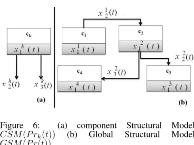
Strucural Model
The component structural model CSM(P rk(t)) is
de-signed as an abstract generic hydraulic component making a relation between an input flow xk1, xk2 and
xk3 (cf. Figure 6 a). The Global structural model
GSM(P (t)) is a 3-tuple < COM P S, Rp, Rx > (cf.
Figure 6 b) where:
• COM P S={c1, c2, c3, c4} is the finite set of
con-stants denoting the system components,
• Rp is a set of equality predicates
defin-ing the interconnections between the compo-nents. Rp={out(c1)=in(c2), out1(c2)=in(c3),
out2(c2)=in(c4)}
• Rx is a set of equality predicates linking
each variable. Rx={ out(c1)=x21, out(c3)=x31,
out(c4)=x41, out1(c2)=x22, out2(c2)=x23}.
Figure 6: (a) component Structural Model CSM(P rk(t)) (b) Global Structural Model
23ndInternational Workshop on Principles of Diagnosis Cx 1 1 1 ={(x 1 1,0)} C x1 1 2 ={(x 1 1,1)} C x1 1 3 ={(x 1 1, 2)} Cx 1 2 1 ={(x 1 2,0)} C x1 2 2 ={(x 1 2,1)} C x1 2 3 ={(x 1 2,2)} Cx 2 1 1 ={(x 2 1,0)} C x2 1 2 ={(x 2 1,1)} C x2 1 3 ={(x 2 1, 2)} Cx 2 2 1 ={(x 2 2,0)} C x2 2 2 ={(x 2 2,1)} C x2 2 3 ={(x 2 2,2)} Cx 2 3 1 ={(x 2 3,1)} C x2 3 2 ={(x 2 3,2)} Cx 3 1 1 ={(x 3 1,0)} C x3 1 2 ={(x 3 1,1)} C x3 1 3 ={(x 3 1,2)} Cx 4 1 1 ={(x 4 1,1)} C x4 1 2 ={(x 4 1,2)}
Table 2: The Timed Observation Classes
Functional Model
A functional model F M is a 3-tuple <∆, F , Rf >
where∆ is the set of values assumable by the different variables (∆x1
1={2, 1, 0}for example), F is a set of
functions define the relation between variables. Two types of relations are defined :
• Relation between the different variables of the same component are : f4(x11) = x
1 2, f5(x21) = x 2 2, f6(x21) = x 2
3that determine the CF M ;
• Relation between the different variables belong-ing to different components are: f1(x12) = x
2 1, f2(x23) = x 4 1, f3(x22) = x 3
1 that determine the
GF M ; behavior Model
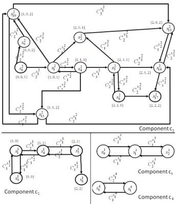
The set of system observation classes derived are given in Table 2 and the set of states of the pipe, for example, are represented in Table 3 (we represent only the sates physically possible using the hydraulic T.o.S). Figure
States x2 1 x 2 2 x 2 3 States x 2 1 x 2 2 x 2 3 s2 0 0 0 1 s 2 1 1 0 1 s2 2 2 0 1 s 2 4 1 1 1 s2 5 2 1 1 s 2 8 2 2 1 s2 9 0 0 2 s 2 10 1 0 2 s2 11 2 0 2 s 2 13 1 1 2 s2 14 2 1 2 s 2 17 2 2 2
Table 3: The pipe states
7 shows a graphic representation of the behavior model of the different components of the hydraulic system. The state transition function defines state s2
2as the next
state when the system is in state s2
1and an occurrence of the Cx 2 1 3 occurs (i.e. γ(s 2 1, C x2 1 3 ) = s 2 2). Diagnosis
Let us consider the sequence of timed observation ω = { ox2 2(t0) ≡ (1, t0), ox 3 1(t0) ≡ (1, t0), ox 2 3(t1) ≡ (2, t1), ox4 1(t1) ≡ (2, t1), ox 2 2(t2) ≡ (0, t2) ,ox 3 1(t2) ≡ (0, t2) , ox2
1(t3) ≡ (2, t3)} (We consider that ti≤ ti+1).
The application of the Algorithm defined in Figure 4 following the following steps,
Step 1 : Compute the set of timed observations at t= tk
The result of this step is given in table 4 (where φ means that there is no change of the variable value in
Figure 7: behavior Model of the hydraulic system
ti) t=tk/cj ω1(k) ω2(k) ω3(k) ω4(k) t0 φ {(x 2 2, 1)} {(x 3 1, 1)} φ t1 φ {(x 2 3, 2)} φ {(x 4 1, 2)} t2 φ {(x 2 2, 0)} {(x 3 1, 0)} φ t3 φ {(x 2 1, 2)} φ φ Table 4: Cutting observations
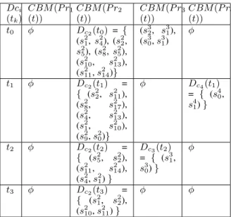
Step 2 : Compute Local Diagnosis att= tk
Table 5 gives the local diagnosis of c1, c2, c3 and
c4 components whose TOM4D component
behav-ior Model are respectively denoted CBM(P r1(t)),
CBM(P r2(t)), CBM (P r3(t)) and CBM (P r4(t)).
For example, let us consider the pipe (c2)
compo-nent. At t = t0, the x22 variable assumes the new
value 1 marking a state transition in the pipe. Con-sidering its Behavior Model CBM(P r2(t)) (cf.
fig-ure 7), the possible states of c2 after the occurence
of a the class Cx
2 2
2 are defined with the state vector
(x2
1 = φ, x 2
2 = 1, x 2
3 = φ) (where φ denote any
value), that is to say s2 4, s 2 5, s 2 5, s 2 13and s 2 14. Because
only these states have an input arrow labelled with the class Cx
2 2
1 , the possible state before the occurrence of a
timed observation of this class are respectively s2 1, s 2 2, s2 8, s 2 10and s 2
11. As a consequence, the possible State
path (and the local diagnosis) for the c2component at
time t = t0 are Dc2(t0) = { (s 2 1, s 2 4), (s 2 2, s 2 5), (s 2 8, s2 5), (s 2 10, s 2 13), (s 2 11, s 2
14) ˙The same reasoning is made
Dci CBM(P r1CBM(P r2 CBM(P r3CBM(P r4 (tk) (t)) (t)) (t)) (t)) t0 φ Dc2(t0) = { (s21, s 2 4), (s 2 2, s2 5), (s 2 8, s 2 5), (s2 10, s 2 13), (s2 11, s 2 14)} (s32, s 3 1), (s30, s 3 1) φ t1 φ Dc2(t1) = { (s2 2, s 2 11), (s28, s 2 17), (s24, s 2 13), (s21, s 2 10), (s29, s 2 0)} φ Dc4(t1) = { (s4 0, s41)} t2 φ Dc2(t2) = { (s2 5, s 2 2), (s2 11, s 2 14), (s2 4, s 2 1)} Dc3(t2) = { (s3 1, s3 0)} φ t3 φ Dc2(t3) = { (s2 1, s 2 2), (s2 10, s 2 11)} φ φ
Table 5: Local Diagnosis for different component
Step 3 : Compute Global Diagnosis att= tk
In the running example, at t= t0, the possible states of
the components are given in Table 6. No information
COM P S possible state possible state COM P S occupied at t < t0 occupied at t= t0
c1 φ φ c2 s 2 1, s 2 2, s 2 8, s 2 10, s 2 11 s 2 4, s 2 5, s 2 5, s 2 13, s 2 14 c3 s 3 1 s 3 1 c4 s 4 0 s 4 0
Table 6: Possible states occupied by the different com-ponents at t∈ ]t0, t1]
about the c1state. The possible state occupied by c1
is the set of possible states of c1. The global diagnosis
D(t1) is concerned with 4 × 4 × 2 × 1 = 32 possible
paths of different components. We use the functional model to eliminate the physically impossible states and to ensure consistency between the S-Paths calculated for example, only s1
(x1 2) = s
2
(x2
1) are kept (f4
de-fined in the functional model as the identity function (∀ t, x1
2(t) = x 2
2(t) ). Only the state s 1
4 is consistent
with the possible states of c1 at t0. Doing so lead we
define the global diagnosis D(ti) in different instance
for example D(t0)={ (s14∧ s 2 4∧ s 3 1∧ s 4 0)∨ (s 1 4∧ s 2 5 ∧s3 1∧ s 4 0, (s 1 4∧ s 2 13∧ s 3 1∧ s 4 0), (s 1 4∧ s 2 14∧ s 3 1∧ s 4 0) }
Step 4 : concatenation operation
The definition 8 is used to merge all global diagnosis calculated at t < tk. The final global diagnosis
re-sulting the concatation of D(ti) a different instance :
D(t < t0), D(t0),D(t1),D(t2)→ D(t3) is D(t3) ={(s11 ∧ s2 11∧ s 3 0∧ s 4 1)} 6 CONCLUSION
We have shown that Timed Observation Theory (and TOM4D in particular) are suitable techniques for
model-based diagnosis and for studying diagnostic properties of dynamic systems. To the best of our knowledge, similar approaches have been considered in (Cordier and Grastien, 2007), (Baroni et al., 1999) and (Console et al., 2000) . A Comparison between PEPA, D.E.S approach and TOM4D is made in (Fakhfakh et al., 2012b) . What we presented can be regarded as a preliminary work since we have not exploited all the potentialities of the theory. In particular, we will investigate how more complex properties concerning diagnosis can be defined and verified within our approach.
A problem can be discussed when we have two timed observations corresponding to one component are simultaneous (came on the same instance tk). In
fact, two timed observations are associated to two ob-servation classes in the same instance. Consequently, the consistance with the CBM and the set of observa-tions (such that we have defined in the article) is not possible. Hence, another extension of our algorithm is important to support the timed observations simultane-ous.
ACKNOWLEDGMENTS
The authors would like to thank the Provence Alpes -Cˆote d’Azur R´egion and FEDER (Fonds Europ´een de DEveloppement R´egional) for their funding.
REFERENCES
(Baroni et al., 1999) P. Baroni, G. Lamperti, P. Pogliano, and M. Zanella. Diagnosis of large active systems. In Artificial Intelligence 110, pages 135–183, 1999.
(Chittaro et al., 1993) L. Chittaro, G. Guida, C. Tasso, and E Toppano. Functional and teological knowl-edge in the multi-modeling approach for reasoning about physical systems: A case study in diagnosis. In IEEE Transactions on Systems, Man, and
Cyber-netics, 23(6), pages 1718–1751, 1993.
(Console et al., 2000) L. Console, C. Picardi, and M. Ribaudo. Diagnosing and diagnosability anal-ysis using pepa. In 14th European Conference on
Artificial Intelligence, 2000.
(Cordier and Grastien, 2007) M.-O. Cordier and A. Grastien. Exploiting independence in a decen-tralised and incremental approach of diagnosis. In
20th International Joint Conference on Artificial Intelligence, 2007.
(Fakhfakh et al., 2012a) I. Fakhfakh, M. Le Goc, L. Torres, and C. Curt. Modeling and diagnosis characterization using timed observation theory. In
7th International Conference on Software and Data Technologies, ICSoft, 2012.
(Fakhfakh et al., 2012b) I. Fakhfakh, M. Le Goc, L. Torres, and C. Curt. Modeling dynamic systems for diagnosos: Pepa/tom4d comparison. In 14th
In-ternational Conference on Enterprise Information Systems, ICEIS, 2012.
(Le Goc, 2006) M. Le Goc. Notion d’observation pour le diagnostic des processus dynamiques : ap-plication sachem et `a la d´ecouverte de connais-sances temporelles. In Universit´e Aix-Marseille
23ndInternational Workshop on Principles of Diagnosis
III - Facult´e des Sciences et Techniques de Saint J´erˆome, 2006.
(Rosenberg and Karnopp, 1983) R. Rosenberg and D. Karnopp. Introduction to physical system dy-namics. In McGraw-Hill, Inc. New York, NY, USA., 1983.
(Schreiber et al., 2000) Th. Schreiber, J. M. Akker-mans, A. A. Anjewierden, R. de Hoog, N. R. Shad-bolt, W. Van de Velde, and B. J. Wielinga. Publica-tion, knowledge engineering and management the commonkads methodology. MIT Press, 2000. (Zanni et al., 2006) C. Zanni, M. Le Goc, and C.
Fry-dmann. A conceptual framework for the analysis, classification and choice of knowledge-based sys-tem. In International Journal of Knowledge-based
and Intelligent Engineering Systems, 10, pages 113–138. Kluwer Academic Publishers, 2006.