HAL Id: halshs-00161572
https://halshs.archives-ouvertes.fr/halshs-00161572
Submitted on 31 Mar 2009HAL is a multi-disciplinary open access archive for the deposit and dissemination of sci-entific research documents, whether they are pub-lished or not. The documents may come from teaching and research institutions in France or abroad, or from public or private research centers.
L’archive ouverte pluridisciplinaire HAL, est destinée au dépôt et à la diffusion de documents scientifiques de niveau recherche, publiés ou non, émanant des établissements d’enseignement et de recherche français ou étrangers, des laboratoires publics ou privés.
The Emergence of Coordination in Public Good Games
Walid Hichri, Alan Kirman
To cite this version:
Walid Hichri, Alan Kirman. The Emergence of Coordination in Public Good Games. European Physical Journal B: Condensed Matter and Complex Systems, Springer-Verlag, 2007, 55 (2), pp.149-159. �halshs-00161572�
The Emergence of Coordination in Public Good Games
Walid HICHRI(GREQAM & University of Aix-Marseille III) &
Alan KIRMAN*
(IDEP-GREQAM, EHESS, IUF & University of Aix-Marseille III)
This version December 2006
Abstract:
In physical models it is well understood that the aggregate behaviour of a system is not in one to one correspondence with the behaviour of the average individual element of that system. Yet, in many economic models the behaviour of aggregates is thought of as corresponding to that of an individual. A typical example is that of public goods experiments. A systematic feature of such experiments is that, with repetition, people contribute less to public goods. A typical explanation is that people “learn to play Nash” or something approaching it. To justify such an explanation, an individual learning model is tested on average or aggregate data. In this paper we will examine this idea by analysing average and individual behaviour in a series of public goods experiments. We analyse data from a series of games of contributions to public goods and firstly to see what happens, if we follow the standard approach and test a learning model on the average data. We then look at individual data, examine the changes that this produces and see if some general model such as the EWA (Expected Weighted Attraction) with varying parameters can account for individual behaviour. We find that once we disaggregate data such models have poor explanatory power. Groups do not learn as supposed, their behaviour differs markedly from one group to another, and the behaviour of the individuals who make up the groups also varies within groups. The decline in aggregate contributions cannot be explained by resorting to a uniform model of individual behaviour.
Key Words: Experimental Economics, Public Goods, Learning models, Individual and Aggregate
behaviour.
PACS numbers: 05.65 +b, 07.05, 02.50. * Corresponding author:
Centre de la charité, 2 rue de la charité 13002, Marseille, France. Tel. : +33 4. 91. 14. 07. 51. or + 33 4. 91. 14. 07. 70.
Fax number: +33 4 91 90 02 27 e-mail: kirman@ehess.univ-mrs.fr
1. Introduction
The topic of this paper is one which is central to economics. We frequently build models based on hypotheses about individuals’ behaviour and then test these on aggregate behaviour. The assumption is that the aggregate can reasonably be taken to behave like an individual. Thus, if we cannot reject our individual based model at the aggregate level, then we conclude that it is a valid model of how people are behaving. We will examine data from a series of experiments on contributions to public goods and show that while the average behaviour seems to correspond to a reasonable individual model, neither the groups nor the individuals playing the game do so.
Public goods games are useful in this respect since we have some well established stylised facts concerning them. Indeed, there is a wealth of information from public goods experiments showing that, with respect to the Nash equilibrium of the one-shot game people initially over-contribute to public goods but that, with repetition, they over-contribute less. Although these experiments have too few rounds, in general, to make meaningful statements about the “convergence” of the total contributions they do decline towards the Nash equilibrium. What the players in these experiments are faced with is a finite repeated game which can be solved by backward induction. The solution in the standard linear model is one of a dominant strategy in which people contribute nothing. However, it is well established that this is not what actually happens. Indeed since individuals do not play in this way from the outset, we cannot attribute the observed behaviour to that associated with an equilibrium of the finite repeated game. Furthermore players do not establish the cooperative, or socially optimal outcome and indeed, in general, move collectively away from such a solution. So, a typical explanation, for the observed behaviour, is that people “learn to play Nash” or something approaching it. In this paper we will examine this idea by analysing average and individual behaviour in a series of public goods experiments.
There are two very different views of learning in games. Population learning suggests that the configuration of strategies in a population game will converge towards some limit, which may or may not be a solution of the one-shot game. How this happens is explained typically by
arguing either that a certain proportion of players will adopt strategies which are performing better than average, or that some of the players will be replaced by others ,who are identified with more successful strategies. This literature does not discuss the mechanism that leads to the expansion of successful strategies nor that which cause less successful strategies to fade. But this is the sort of idea invoked in literature where some classified certain people, from their behaviour, as Nash and found that at the beginning of their public goods experiments 50% of players were Nash and, at the end 69% fell into this category. This makes it tempting to believe that the population was evolving towards Nash. But this raises an important question. Is it true that that the people who switched had “learned to play Nash”, and if so, how and why?
This last question suggests a second and very different approach which is to model the individual learning process and to see if observed behaviour, particularly that in experiments, corresponds to such a model. Here again there is a distinction to be made. One approach is to assume that all individuals learn in the same way and then to test the learning model on the average observed data (see Erev and Roth [1]). This is very common practice and often gives rise to rather convincing results. However, as Camerer et al. [2] point out, the estimated parameters for the representative individual may not coincide with the average parameters of the population. Furthermore, this approach is fundamentally flawed. To assume that the average player behaves in a certain way is to give way to the same temptation as that offered by the “representative agent” in macroeconomics. It is not, in general logically consistent to attribute the characteristics of an individual to average behaviour, even if all the underlying individuals obey the assumptions made about their behaviour. If all the individuals were indeed identical then this objection could be overruled, but in this case, how do we know, if we reject the model, whether we are rejecting the model itself, or the hypothesis that all agents are identical?
An alternative approach is to assume that individuals behave according to the same learning model but differ in their parameters. This is the approach adopted, for example, by Camerer et al. [2]. In this case one must try to find a model that is general enough to encompass a number of basic learning rules and this is indeed, the goal of the “experience weighted attraction” model (E.W.A.) used by the authors just mentioned and introduced by Camerer and Ho [3]. This avenue is appealing for a number of reasons. It allows for heterogeneity among the agents and
also allows one to detect whether there are clusters of players who concentrate around some of the special cases covered by the general model. There are two such fundamental classes of rules: those which focus on learning from experience, in the sense of reinforcement and those which focus on anticipating what opponents will do, given their previous behaviour. There are two classic classes of rules which, were previously considered as rival .The first of these are the “reinforcement” models in which strategies are updated on the basis of their results in the past,(an approach based on the work of Bush and Mosteller [4], see e.g. Roth and Erev [5] and Mookerjhee and Sopher [6]). The second are the so-called ``belief'' models in which agents update their anticipation of their opponents' behaviour on the basis of their previous behaviour, fictitious play being a good example (see e.g. Fudenberg and Levine [7]). Both of these classes are included within the EWA learning rule. However, it is worth noting that the basis of EWA is still exclusively backward looking and nothing is said about how agents might learn to reason in a forward looking way. Thus although rather general, it could be argued that EWA is still not general enough. However the difficulty of finding a rule which also encompasses this sort of learning is clear. Camerer [8] and Camerer et al. [9] are pursuing work in this direction.1
Another possibility is not to find a rule which encompasses others as special cases but to allow for different rules and simply to try, on the basis of observed behaviour, to assign agents to rules. This is the procedure followed by Cheung and Friedman [10], Stahl [11] and Broseta [12]. There are at least two problems with this sort of approach. Firstly, the rules specified are necessarily arbitrarily chosen, and secondly, the tests are not very powerful since, in such situations, the number of observations is, in general, not very large.
Our objective in this paper is to analyse data from a series of games of contributions to public goods and firstly to see what happens, if we follow the standard approach and first determine the trend of contributions and then test a learning model on the average data. We next look at group and then individual data, examine how this changes the results and see if some general model such as the EWA with varying parameters can account for individual behaviour. Our case is rather favourable for this sort of test since, by telling agents how much was
contributed to the public good in total, at each step, we allow them to know how much they would have obtained from foregone strategies. This avoids a fundamental problem raised by Vriend [13] as to how agents can update the weight they put on strategies which they have not played if they do not know how much these would have paid. We find that, nevertheless, behaviour differs across groups and individual behaviour is not easily categorized.
It is worth recalling that, in this type of experiment, individuals are divided into groups who play the game for a fixed number of periods. Thus the groups are unaffected by each others’ behaviour. Yet the whole population seems to learn in a simple way, while the separate groups do not learn as supposed, and their behaviour differs markedly from one group to another. Furthermore, behaviour of the individuals who make up the groups also varies within those groups.
The usual explanation for some of the discrepancies in strategies in the early rounds of public goods games, as Ledyard [14] explains, is that confusion and inexperience play a role. Indeed, this is one of the basic reasons why repetition has become standard practice in these experiments. Yet, as we will see, this would not be enough to explain some of the individual behaviour observed in our data.
We will now turn now to the particular choice of model made for the experiments and the rest of the paper will be structured as follows. Firstly we will explain the particular features of our model and their advantages. Then we will give the details of the experiments we ran. We will then describe the data from the experiments. In the following section we will perform some simple tests on the average data for the whole population, for the group averages and finally for the individuals. Having pointed out the differences between these, we proceed to an analysis of the performance of the EWA rule on individual data and compare this with our previous results. We then conclude.
2.1. The basic public goods game:
In the basic game of private contribution to a public good, each subject i, (i=1,..,N) has to split an initial endowment E into two parts: the first part (E - Ci) represents his private share and the other part Ci represents his contribution to the public good. The payoff of each share depends on and vary with the experimental design, but in most experiments is taken to be linear (Andreoni [15]). The total payoff π i of individual i, in that case is given by the following expression:
∑
=+
−
=
N j j i iE
c
c
1θ
π
This linear case gives rise to a corner solution. In fact, assuming that it is common knowledge that players are rational payoff maximisers, such a function gives a Nash equilibrium
(N.E.) for the one shot game at zero and full contribution as social optimum (S.O.). The dominant
strategy for the finite repeated game, is to contribute zero at each step. Nevertheless, experimental studies show that there is generally over-contribution (30 to 70% of the initial endowments) in comparison to the N.E.
Attempts to explain this difference between the theoretical and the experimental results are the main subject of the literature on private contribution to public goods. To do so, several pay-off functions with different parameters have been tested in various contexts to try to see the effect of their variation on subjects’ contributions (for surveys, see Davis and Holt [16], Ledyard [14] and Keser [17]).
In the linear case, given that the N.E. is at zero, and giving that subjects could not contribute negative amounts to the public good, error can only be an over-contribution. To test the error hypothesis experimentally, Keser [18] performed a new experiment. She proposed a new design in which the payoff function is quadratic and the equilibrium is a dominant strategy in the “interior of the strategy space.” With such a design, undercontribution becomes possible and error on average could be expected to be null. The results of Keser's experiment show that in each period, contributions are above the dominant solution, which leads to the rejection of this error hypothesis.
Another way to introduce an interior solution is to use a linear payoff for the private good and a concave function for the public one. Sefton and Steinberg [19] compare these two possible payoff structures. They call the first one “the Dominant strategy equilibrium treatment” and the second “the Nash equilibrium treatment.” The results show that “average donations significantly exceed the predicted equilibrium under both treatments, falling roughly midway between the theoretical equilibrium and optimum... Donations are less variable under the dominant strategy equilibrium treatment than under the Nash equilibrium treatment.”
2.2. Our Model:
The theoretical model and design used for the experiments we report in this paper are those used in Hichri [20] and concern a public goods game with a “Nash equilibrium treatment” [19]. The individual payoff function is
1 / 2 1
(
)
i i N E c j jc
π
= − +θ
=∑
The Nash equilibrium (N.E.) and the social optimum (S.O.), also called Collective Optimum (C.O.) corresponding to this payoff structure are not trivial solutions but in the set of the possible choices. The Nash equilibrium for individuals is not a dominant strategy for the finite repeated game. Indeed the solution for that game poses problems for a simple reason. There is a unique Nash equilibrium in the sense that for any Nash equlibrium the group contribution is the same. However, that contribution can be obtained by several combinations of individual contributions. Since there are many Nash equilibria for the one-shot game, precisely what constitutes an equilibrium for the repeated game is unclear. Calculations show that for a group of
N subjects, at the C.O., the total contribution is given by the following expression:
2 _ _ _ 2 1 . 4 N i i y N
Y
θ = = = ∑
and at the N.E. is equal to:2
* *
.
4
Y
=
N
y
=
θ
where y* is the symmetric individual Nash equilibrium.
With such a design, the Nash equilibrium and the social optimum vary with the value of θ. We shall see whether there is any difference between the evolution of indivdual and aggregate contributions under the different treatments.and how well learning models explain this evolution.
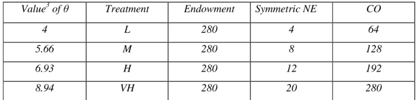
The original purpose of the experiments, from which the data is used here, was to test the effect on the level of the social optimum and of the Nash equilibrium of varying θ. Clearly θ may be considered as a measure of the productivity of the process which transforms the private into the public good. The marginal value of an individual contribution varies positively with θ. To test if modifying θ has, in fact, an impact on contributions, we gave it four different values, which gives four levels for the social optimum (C.O.). By varying this value, we vary then the C.O. and the N.E. levels. The following tables summarize for each of the four treatments (Low, Medium, High and Very High, named respectively L, M, H and V.H.) the different levels of interior solutions for each group of four (N=4) persons (table 1) and for one subject2 [21] in each group (table 2):
Value3 of θ Treatment Endowment Symmetric NE CO
4 L 280 4 64
5.66 M 280 8 128
6.93 H 280 12 192
8.94 VH 280 20 280
Table 1: The NE and the CO values for the four treatments for one group.
2 An analysis of the experiment at the individual level is presented in Hichri [21]. 3
These are approximate values. The exact values are respectively : 4 , 5.6568542 , 6.9282032 and 8.9442719. We choose these values such that the C.O. corresponds respectively to 64 , 128 , 192 and 280.
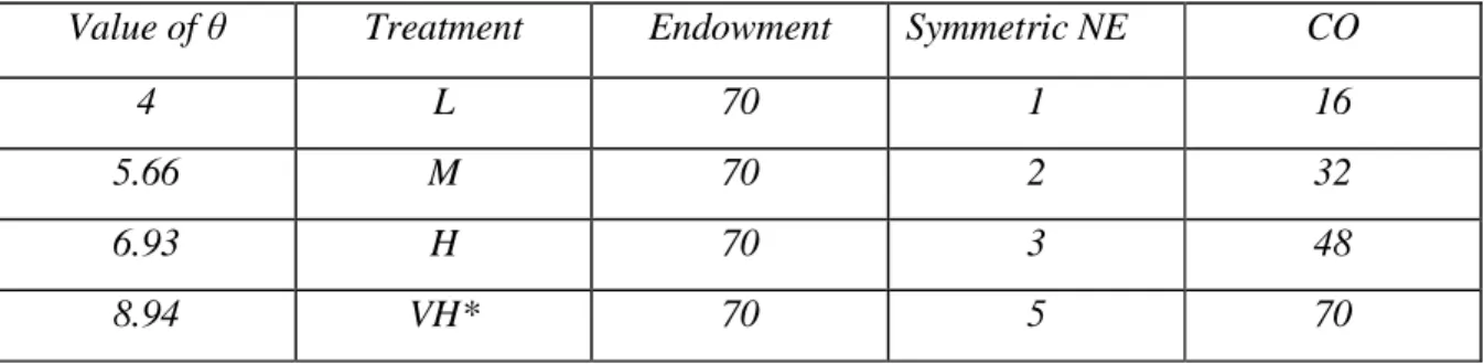
Value of θ Treatment Endowment Symmetric NE CO
4 L 70 1 16
5.66 M 70 2 32
6.93 H 70 3 48
8.94 VH* 70 5 70
Table 2: The symmetric NE and the CO values for the four treatments for one subject.
The set of possible group contributions in our model is very large. In fact, given that each one of the four individuals of a group is endowed with 70 tokens, each group can contribute an amount that varies between zero and 280.
We then added two other features and we again looked not only at the effect of variations in θ but also at the variability of individual behaviours. In the first variant, we replicated the same experiment as before with the introduction of promises before the decision period relative to the contribution to the public good. The four treatments with promises are called L.P., M.P., H.P. and
V.H.P.
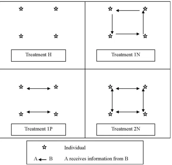
In the last experiment, we introduce as a parameter the information about the contribution of some members of one group to the public good. Three treatments were compared to the treatment H. This treatment is used as a benchmark (no-information treatment) and is chosen because it allows us to keep the C.O. in the interior of the strategy space but, at a high level. The three new treatments with information are “one neighbor”, “one partner” and “two neighbors” (respectively called 1.N., 1.P. and 2.N.) and have the same theoretical design as treatment H (same C.O. and N.E.). In fact, information is introduced after the end of the one-shot game and has no effect on the theoretical solutions.
While in treatment H individuals are informed only of the sum of contributions of their group, in treatment 1.N. each one of the four individuals in a group knows at the end of each period the contribution of his right neighbour, in addition to the sum of contributions of the group. In treatment 1.P., each two individuals in one four persons group exchange information
about their own contributions. These Partners are the same for all the periods of the game. Finally, in the last treatment (2.N.), for each individual information concerns two Neighbours, the right one and the left one. The following figure (figure 1) depicts these four treatments:
In all treatments, and from a period to another, information given to individuals concerns always the same persons.
The data of these three new treatments is also used to test the learning models at the population, group and individual level. This allows us to see whether the results in our reference framework are robust to different “institutional frameworks.”
The following section presents the experimental results relative to the four treatments of both experiments with (treatments L.P., M.P., H.P. and V.H.P.) and without (treatments L, M, H and V.H.) promises and those of the three new treatments with information (treatments 1.N., 1.P. and 2.N.).
Note that the total number of treatments is 11. Each one is played by six independent groups of four persons and for 25 periods, which means that each treatment is played by 24 individuals. The total number of players is then 264 ( 96 of them have played four treatments without promises, 96 have played four treatments with promises and 72 have played the same treatment but with different information).
3. The experimental results
Our initial analysis will be at the aggregate level where we have for each treatment the average contribution of the six groups compared to the aggregate N.E. and to the aggregate C.O. These results are reported in figures 2 for the four treatments without promises, in figures 3 for the four treatments with promises and in figure 4 for treatments with information.
3.1. Basic results without promises:
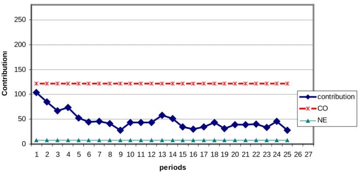
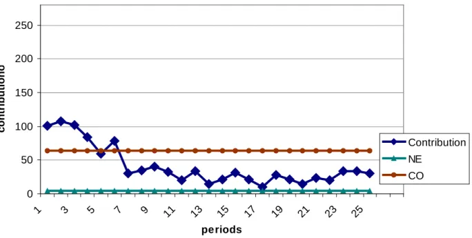
The first thing we observe when analysing the experimental results is the fact that the average group contribution (Y) decreases over time. In fact, the Very High treatment (θ= 8.94), has 133.33 and 91.5 as values of the first and the last periods (see figure 2). In the case of
treatments H and M, the average group contribution (Y) decreases during the 10 first periods and stays at a steady level during the rest of the periods of the game. In the last treatment L, this average group contribution starts at 67.67 and decreases steadily during the 25 periods of the game until finishing at 7.16. The decrease of contributions is however less evident in treatment
V.H. Generally, if we do not consider the first five periods that could be assimilated to “learning periods,” contributions are almost steady over the twenty last periods for treatments M, H and V.H.
Our results show that contributions vary with the collective optimum (C.O.) level. There is overcontribution in comparison to the N.E. This overcontribution increases with the C.O. level in absolute value. Nevertheless, average contributions remain proportionately as far from the
C.O. as the level of the latter gets high. Computing these contributions in relative values by
calculating an overcontribution index that takes into account the N.E. and the C.O., shows that, except in treatment V.H., this ratio is constant.
That means that an increase the C.O. level leads to, a proportional increase in individual and hence, total contributions.
In treatment L, the average group contribution seems to decrease and to tend steadily to the N.E. value (which is 4). For this treatment, where the C.O. level is very low, subjects seem to tend to the theoretical predicted value for the one-shot game. The difference between the theoretical prediction and the experimental results is less evident in this framework as the game proceeds and indeed, such a result is rarely observed in the experimental literature relative to public goods. It seems somewhat paradoxical that subjects contribute less and learn to play the NE value when the C.O. is low. For this is precisely the case in which the C.O. is easy to reach in the sense that it does not require a large contribution. For high levels of the C.O., it is, in fact, risky for one subject to cooperate and to try to reach the social optimum by contributing a large amount to the public good. Taking such a risk can lead one subject to share his or her contribution with other subjects that choose not to contribute, and, in so doing, to lose, most of his or her private payoff. Thus the risk when faced with “free riding” behaviour is higher as the
total contribution in the VH treatment without promises 0 50 100 150 200 250 1 2 3 4 5 6 7 8 9 10 11 12 13 14 15 16 17 18 19 20 21 22 23 24 25 26 27 periods C o n tr ib u ti o n n n Contribution CO NE
Total contribution in the H tratment without promises
0 50 100 150 200 250 1 2 3 4 5 6 7 8 9 10 11 12 13 14 15 16 17 18 19 20 21 22 23 24 25 26 27 periods C o n tr ib u ti o n n n CONTRIBUTION CO NE
Total contribution in the M treatment without promises 0 50 100 150 200 250 1 2 3 4 5 6 7 8 9 10 11 12 13 14 15 16 17 18 19 20 21 22 23 24 25 26 27 periods C o n tr ib u ti o n n n contribution CO NE
total contribution in the L treatment without promises
0 50 100 150 200 250 1 3 5 7 9 1 1 1 3 1 5 1 7 1 9 2 1 2 3 2 5 2 7 periods C o n tr ib u ti o n n n Contribution NE CO
The other side of the coin is that the gains to be had from contributing more collectively are higher when the C.O. is higher. One natural interpretation of some individual behaviour is that individuals make generous contributions initially to induce others to do the same. This is, of course, not consistent with optimising non-cooperative behaviour but has been evoked in considerations of non-equilibrium behaviour.
3.2. Results with promises:
Promises are introduced in the public goods game as step preceding real contributions. In each group, and in each period, individuals are asked to announce their intentions as how much they will effectively contribute in the considered period. The sum of these intentions is revealed to the members of the group. Thus this information become common knowledge before the beginning of real game where individuals announce their effective contributions that will be considered when calculating their gains. Intentions are considered as promises that are “cheap talk,” seeing that the gains are not affected by the introduction of promises. Also, the N.E. and the
C.O. of the game are the same than in the game without promises.
As expected, and in concordance with findings in experimental literature, the introduction of promises increases contributions to the public good, although this increase is not very marked. Consequently, the average group contributions are closer to the Nash equilibrium in treatments without promises.
What is interesting from our point of view is that the main difference between treatments with promises and those without promises is obviously the heterogeneity of groups and individuals behaviour when promises are allowed. In fact, the data permits to isolate in treatments with promises different strategies that does not exist in treatments without promises.
Total contribution in the VH treatment with promises 0 50 100 150 200 250 1 3 5 7 9 11 13 15 17 19 21 23 25 periods C o n tr ib u ti o n n n Contribution NE CO
Total contribution in the H tratment with promises
0 50 100 150 200 250 1 3 5 7 9 11 13 15 17 19 21 23 25 periods C o n tr ib u ti o n n n Contribution CO NE
Total contribution in the L treatment with promises 0 50 100 150 200 250 1 3 5 7 9 11 13 15 17 19 21 23 25 periods c o n tr ib u ti o n o n Contribution NE CO
Total contribution in the M treatment with promises
0 50 100 150 200 250 1 3 5 7 9 11 13 15 17 19 21 23 25 periods c o n tr ib u ti o n o n Contribution NE CO
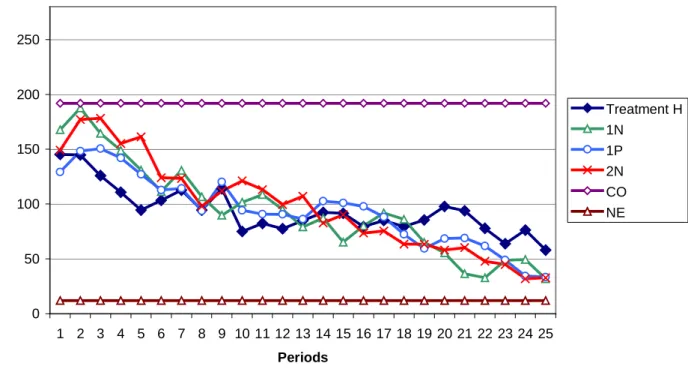
3.3. Results with Information:
While the introduction of promises increases contributions to the public good, information about the contribution of the other members of one group seems to have no effect on the decision of contribution of individuals. In fact, as shown in the following figure (figure 4), where we represent average total contribution for the three treatments with information and for treatment H (already given in figure 2), the experimental results show that there is no difference between contributions with information and contributions without. The aggregate behaviour is very similar in the four treatment: overcontribution is evident during all the experiment and decreases over time, as contributions become closer to the N.E.
0 50 100 150 200 250 1 2 3 4 5 6 7 8 9 10 11 12 13 14 15 16 17 18 19 20 21 22 23 24 25 Periods A v e ra g e C o n tr ib u ti o n Treatment H 1N 1P 2N CO NE
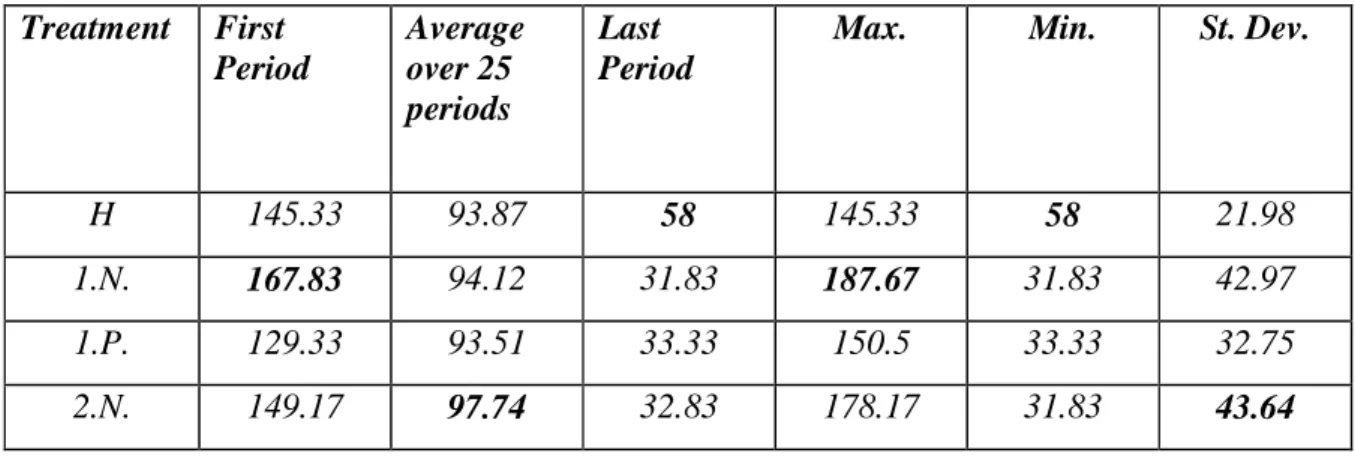
Note that in all treatments, contributions start by increasing and are very close to the C.O. in the first periods of the game. Also, average total contribution is almost the same for three of the four treatment in the last period. Table 3 summarises the results for these four treatments:
Treatment First Period Average over 25 periods Last Period
Max. Min. St. Dev.
H 145.33 93.87 58 145.33 58 21.98
1.N. 167.83 94.12 31.83 187.67 31.83 42.97 1.P. 129.33 93.51 33.33 150.5 33.33 32.75 2.N. 149.17 97.74 32.83 178.17 31.83 43.64
Table 3 : Average Total Contribution in treatments H, 1N, 1P and 2N
These results are in concordance with other experiments where information is introduced in some way in a public goods game. For example in Cason and Khan [22], the standard design of a public goods game is compared to a new one where information about group’s contribution is given every 6 periods (imperfect monitoring) in presence of face-to face communication. The authors expected lower contribution levels under imperfect monitoring, but found no difference between both. They also found that communication ensures high levels of contribution under both information treatments.
Generally, information concerns the endowments and payoffs of other members of one group and is tested with heterogeneity (same/different endowments, payoffs…). This is the case in Chan et al. [23] where the authors conclude that information has no significant effect on contributions when subjects are identical (see also Ledyard [14]).
In the following section, we will test a simple learning model both on the aggregate level to see whether this model suits the experimental data and whether it is still available when applied to individuals.
The data that will be used for these tests is the one of treatment H without promises, treatment H with promises and treatments 1.N., 1.P. and 2.N. with information. This choice is based on the fact that all these treatments have the same theoretical payoff function (high level of social optimum). As well, the fact that treatments H with and without promises and treatments with information (1.N., 1.P. and 2.N.) have the same theoretical solutions allows us to compare our experimental data with simulations of learning models without having any bias concerning the eventual difference between both results.
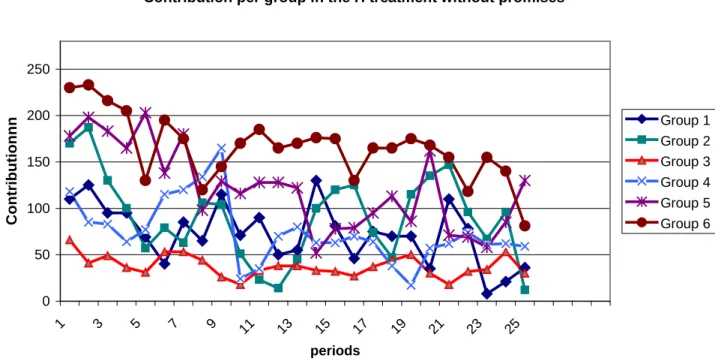
3.4. The group and the individual level:
Although at the aggregate level there is no volatility, In all treatments, there are at the group level different behaviours in the same group and between groups. The latter are not regular and we can clearly identify several ways of contribution. Figure 5 shows the contribution of the six groups in treatment H without promises and gives us an idea about this variation between groups.
Contribution per group in the H treatment without promises
0 50 100 150 200 250 1 3 5 7 9 11 13 15 17 19 21 23 25 periods C o n tr ib u ti o n n n Group 1 Group 2 Group 3 Group 4 Group 5 Group 6
Within groups, at the individual level, there is also a difference between the individual and the aggregate behaviour. In fact, individuals behave differently. Moreover, the individual behaviour is more difficult to classify because of the great volatility of contributions of one subject during the 25 periods of the game.
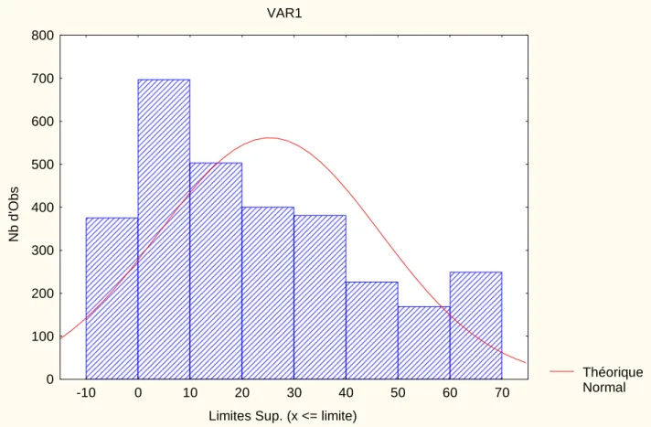
To have an idea about the different levels of contributions of individuals, we classify contributions in 8 intervals of ten each and we present in figure 6 the number of times individuals make a contribution belonging to each interval. As in each of the 5 treatments there are 24 persons playing 25 periods, we have then 3000 observations or decision of contribution. As we can see in figure 6, almost all the intervals are significant:
Figure 6: number of individual contributions for each interval for the 5 treatments (3000 decisions).
Théorique Normal VAR1
Limites Sup. (x <= limite)
Nb d 'O b s 0 100 200 300 400 500 600 700 800 -10 0 10 20 30 40 50 60 70
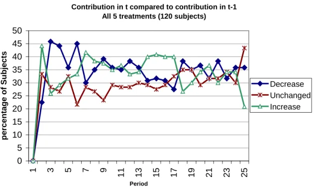
Also, to isolate the different strategies that could explain the individual behaviours, we compare for the 5 treatments and for the 25 decisions of each individual her contribution in period (t) to her contribution in (t-1). This allows us to know whether individuals react in response to past contributions. We classify this comparison into three possibilities: contribution in t increases, decreases and remains unchanged in comparison to contributions in (t-1). Figure
7 shows that all these strategies are significant:
Figure 7: Percentage of increasing, decreasing and unchanged individual contributions in t compared to (t-1) for the 5 treatments (3000 observations).
When we test econometrically for treatment H the model:
We find that θ is significant for the 6 groups while it is not for 13 subjects over 24. Contribution in t compared to contribution in t-1
All 5 treatments (120 subjects)
0 5 10 15 20 25 30 35 40 45 50 1 3 5 7 9 1 1 1 3 1 5 1 7 1 9 2 1 2 3 2 5 Period p e rc e n ta g e o f S u b je c ts Decrease Unchanged Increase t t t
a
C
C
=
+
θ
.
−1+
ε
Also, the assumption
θ
=
θ
i ∀i=1,..,4 is rejected for all the individuals of the 6 groups.Then we can conclude that individuals are heterogeneous.
4. Simple tests of the learning model
After presenting the “Reinforcement Learning model” (R.L.), we will test this simple model at the aggregate level using the experimental data.
4.1. The Reinforcement Learning model:
Two properties of human behaviour in the set of situations we analyse are mentioned in the psychology literature. The first one, known as the “Law of Effect” reflects the fact that choices that have led to good outcomes in the pas are more likely to be repeated. The second one is called the “Power Law of Practice” and announces that learning curves tend to be steep initially, and then flatter. Another property is also observed, which is “recency,” according to which recent experience may play a larger role than past experience in determining behaviour.
There exists a wide variety of learning models in literature. We will use a simple learning model and apply it to our experiments. The model used is the basic reinforcement learning model used for example by Roth and Erev [5]. There are several variations of this model. In the one parameter reinforcement model, each player i, at time t=0, before the beginning of the game, has an initial propensity to play his kth pure strategy. Let
A
ki(
0
)
be this initial propensity. Whena player receives a payoff x after playing his kth pure strategy at time t, his propensity to play strategy k is updated. The rule of updating these propensities from a period to another is given by the following relation:
x
t
A
t
A
i k i k(
+
1
)
=
(
)
+
)
(
)
1
(
t
A
t
A
i k i k+
=
These propensities will allow player i to compute the probability that he plays his kth strategies at time t. Let this probability be
1
e x p (
.
( ) )
( )
e x p (
.
( ) )
i i i k k m j k jA
t
p
t
A
t
λ
λ
==
∑
where the sum is over all of player i's pure strategies j.4
There are several variations on this basic reinforcement learning model, as the cut-off model, the local experimentation model and the experimentation model with forgetting.
4.2. The simple test of the reinforcement Learning at the aggregate level:
We will apply the reinforcement learning model to the aggregate level of the 5 treatments. We divide the set of possible contributions ([0; 280]) into ten equal intervals ([0; 28)]; [29; 56]; [57; 84];…; [252; 280]). At time t = 0, all the possible levels of contribution have the same attraction and the same probability to be chosen.
In period 1, the strategy chosen in the data at the aggregate level receives the payoff x as explained above. At each of the 25 periods, the aggregate contribution of each treatment of one given period played in the real experiment is updated. This model is applied to each of the 5 treatments and the average of these results is calculated and presented in figure 8. This figure shows that the strategy that is played the most according to the reinforcement learning model is to
4 This well known rule is also refereed to as the « Quantal response » rule or the « logit » rule and can be justified as
contribute an amount corresponding to the fourth interval, that is [85;112]. This result corresponds obviously to the experimental data given that we are using this data to update the observed chosen strategies.
Figure 8: The average of probability of playing each of the 10 set of strategies when applying the Reinforcement Learning model to the aggregate level of the six treatments.
0 0,02 0,04 0,06 0,08 0,1 0,12 0,14 1 2 3 4 5 6 7 8 9 10 11 12 13 14 15 16 17 18 19 20 21 22 23 24 25 26 Série1 Série2 Série3 Série4 Série5 Série6 Série7 Série8 Série9 Série10
5. The performance of the EWA rule on individual data
In this section, we will present the “Expected Weighted Attraction” (E.W.A.) Learning model and we will next apply it to the aggregate and the individual level using the same data than the one used in the previous section (the 5 treatments’ data).
5.1. The E.W.A. Learning model:
The details of the “Expected Weighted Attraction” (E.W.A.) model can be found in Camerer and Ho [3,24] and Ho et al. [25]. Suppose N players indexed by i, where i=1,2,...,N. Let
)
( t
A
ij denote the attraction of strategy j for player i once period t is played, where 1, 2,.., ij= m. The Attraction of the different strategies in the E.W.A. learning model are updated differently. The chosen strategies receive an attraction equal to the payoff
π
i player i receives as a result of his choice, while the attractions of the unchosen strategies are updated by adding only a part δ of the foregone payoff. Then, the parameter δ is the weight one player puts on the unchosen strategies.Let
s
ij denote the strategy j of player i, ands
−i(t
)
be the strategies of all players but player i chosen in period t. Attractions of strategies are updated according to the payoffs these strategies provide, but also according to the payoff that unchosen strategies would have provided. The rule of updating attractions in period t is:.
(
1).
(
1)
[
(1
). (
,
( ))].
(
,
( ))
( )
( )
j j j j j i i i i i i iN t
A
t
I s
s
t
s
s
t
A
t
N t
φ
−
− +
δ
+ −
δ
π
−=
I(x,y) is an indicator function that is equal to 1 if x = y and to 0 if not.
π
i(
s
ij,
s
−i(
t
))
is the payoff of player i when he plays strategy j while the other players play the combination of strategiess
−i( t
)
.The parameter φ is a discount factor used to depreciate the previous attractions so that strategies become less attractive over time.
N(t) is the second variable updated in the E.W.A. Learning model. It is the experience
weight used to weight lagged attractions when they are updated. N(t) is updated according to the rule:
1
)
1
(
).
1
(
)
(
t
=
−
N
t
−
+
N
φ
κ
where t≥ 1.The parameter
κ
controls whether the experience weight depreciates more rapidly than the attractions.At t = 0, before the game starts, the two variables
A
ij(t
)
and N(t) have initial values)
0
(
j iA
and N(0).The probability of choosing a strategy j by player i in period (t+1) is calculated by using a logit form: 1
e x p (
.
( ) )
(
1 )
e x p (
.
( ) )
i j j i i m k i kA
t
p
t
A
t
λ
λ
=+
=
∑
where λ controls the reaction of players to the difference between strategies attractions. A low value of λ implies an equal probability for choosing strategies, while a high value supposes that players are more likely to chose strategies with higher attractions.
We note that the reinforcement learning model is a special case of the E.W.A. model. In fact, when φ =1, κ=1, λ=0 and N(0)=1, attractions are updated in the same way than in the
cumulative reinforcement learning model. The E.W.A. learning model includes the reinforcement learning model and other learning models as belief learning as special cases (Camerer and Ho [3]).
5.2. The test of the E.W.A. learning model at the aggregate level :
We ran simulations5 using the same theoretical function as that used in our 5 treatments. We calculate the probability of playing each possible contribution by updating the initial propensities of each strategy using the E.W.A. learning model. The parameters used are those which best fit the model.
First, we play the public goods game 25 periods where the simulation program chooses randomly in the first period one of the 281 possible levels of contribution ([0; 280]). This means that in the first period, all the strategies have the same probability of being chosen. The propensity of the strategy chosen in the first period is updated according to the E.W.A. learning model. Next, the simulation program calculates for each strategy the probability of its being played in period 2. Obviously, the strategy chosen in period 1 has a greater probability of being chosen in period 2. In the second period, the simulation program chooses a new strategy using the new probabilities for being played of each strategy.
This program is run for 25 periods. Figure 9 is an example of 25 strategies belonging to the interval [0; 280] and chosen by the simulation program:
Figure 9: The probability of each of the 25 chosen strategy using the E.W.A. learning model.
We repeat this simulation 1000 times and we calculate the average of the probabilities of all the chosen strategies. The result is presented in figure 10:
Figure 10: The average of the probabilities of 1000 repeated simulation of the 25 periods public goods game using the E.W.A. learning model.
5.3. The test of the E.W.A. learning model at the individual level:
We apply the same simulation program (run 1000 times) for a set of possible strategies that corresponds to the set available to one person playing the public goods game. This set of strategies is [0; 70]. The payoff of one player depends on his strategy but also on the choice of the three other players of the same group who are playing the game. The results are presented in
figure 11:
Figure 11: The average of the probabilities of 1000 repeated simulation of the 25 periods public goods game for one player using the EWA learning model.
5.4. Comparison with the simple learning model :
being played are those who belong to the interval [85; 112]. The results of simulations applied at the aggregate level show that high contributions have the highest probabilities of being played. Obviously, this does not correspond to the experimental findings where low contributions are more likely to be played and where contributions decrease over time.
Simulating the E.W.A. model for single players playing the public goods game shows that contributions belonging to the interval [40; 60] have the highest probabilities of being played
(figure 11). This is not in accordance with the observed strategies. Furthermore, the E.W.A.
model would suggest an essentially monotone evolution. Whilst this is observed at the aggregate level for all treatments, this is far from being the case for the groups and the individuals. The behaviour of players seems to differ widely across individuals and what is more there is no convergence to any common behaviour. Players seem to play out of equilibrium strategies and this does not correspond to any simple learning model.
6. Conclusion :
The simple point made in this paper is that what seems to be rather systematic behaviour at the aggregate level which persists in various treatments of the public goods game, does not reflect such systematic behaviour at the group or individual level. People within groups interact and react to the contributions of the other members of the group. This may lead to very different levels of total contributions across groups and over time. Furthermore, different groups do not necessarily exhibit the uniform decline in total contributions which is observed at the aggregate level across all treatments.
Rather different versions of our basic experiment yield similar results so the difference between the individual and aggregate level cannot be attributed to some specific institutional feature of our experiments.
What it is that causes the variation across indivduals remains an open question. Simplistic explanations such as “degrees of altruism” do not seem to be satisfactory. What does seem to
happen is that some individuals try to signal to others by means of their contribution. They may hope, in so doing, to induce higher payments from their colleagues. If this is what they are doing then they violate some of the simple canons of game theory.
What is clear is that the players do not, in general manage to coordinate on cooperative behaviour. Free riding is something which on average increases over time but many individuals do not follow this pattern. To sum up, the behaviour of individuals varies considerably, but the complexity of the interaction is washed out in the average. Nevertheless, this should not lead us into the trap of attributing individual behaviour to the aggregate nor, and worse, of concluding from the apparent aggregate learning process, that individuals are learning in this way.
References:
1. I. Erev and A. Roth, "Predicting How People Play Games: Reinforcement Learning in Experimental Games with Unique, Mixed Strategy Equilibria", American Economic Review, 88(4), p. 848-881, (1998).
2. C. Camerer, G. Loewenstein, and M. Rabin, Advances in Behavioral Economics, Princeton Univ. Press, (2004).
3. C. Camerer and T. Ho, “Experience-Weighted Attraction learning in normal-form games,” Econometrica, 67, 827-873, (1999).
4. R. Bush, and F. Mosteller, stochastic models for learning, New York: Wiley, (1955).
5. A. Roth, and I. Erev, “Learning in Extensive-Form Games: Experimental Data and Simple Dynamic Models in the Intermediate Term,” Games and Economic Behavior, 8, 164-212, (1995).
6. D. Mookherjee and B. Sopher, “Learning and Decision Costs in Experimental Constant Sum Games,” Games and Economic Behavior, 19, 97-132, (1997).
7. D. Fudenberg and D. Levine, The Theory of Learning in Games, MIT Press, (1998).
8. J. Chong, C. Camerer and T. Ho, “A learning-based model of repeated games with incomplete information,” Games and Economic Behavior (to be published).
9. T. Ho, C. Camerer and J. Chong, “Functional EWA: A One-parameter Theory of Learning in Games, unpublished.
10. Y. Cheung and D. Friedman, “Individual Learning in Normal Form Games: Some Laboratory Results,” Games and Economic Behavior, Elsevier, 19(1), 46-76, (1997).
11. D. Stahl, “Evidence based rules and learning in symmetric normal form games,” International Journal of Game Theory, 28, 111-130, (1999).
12. B. Broseta, “Learning in experimental coordination games: An ARCH approach,” Games and Economic Behavior, 24-50, (2000).
13. N. Vriend, “Does Reasoning Enhance Learning?,” Economics Working Papers 185, Department of Economics and Business, Universitat Pompeu Fabra, 1996.
14. J. Ledyard, “Public Goods: A Survey of Experimental Research,” in J. Kagel, and A. Roth (eds.), The Handbook of Experimental Economics, Princeton University Press, (1995).
15. J. Andreoni, “Cooperation in Public-Goods Experiments : Kindness or Confusion ?,” the American Economic Review, 85(4), Septembre (1995).
16. D. Davis et Ch. Holt, “Experimental Economics,” Princeton University Press, Princeton, N.J, (1993).
17. C. Keser, “Cooperation in Public Goods Experiments,” Scientific Series, CIRANO, (2000).
18. C. Keser, “Voluntary contributions to a public good when partial contribution is a dominant strategy,” Economics Letters, 50, (1996).
19. M. Sefton and R. Steinberg, “Reward structures in public good experiments, Journal of Public Economics, 61, 263-287, (1996).
20. W. Hichri, “Interior Collective Optimum in a Voluntary Contribution to a Public goods Game”, Applied Economics Letters , 11(3), 135-140, (2004).
21. W. Hichri, “Indicvidual Strategies and Aggregate behavior in a public Goods Experiment,” Applied Economics Letters, 13, 969-973, (2006).
22. T. Cason and F. Khan, “A laboratory study of voluntary public goods provision with imperfect monitoring and communication ,” Journal of Development Economics, 58, (1999).
23. K. Chan, S. Mestelman, R. Moir and R. Muller, “Heterogeneity and the Voluntary Provision of Public Goods”, Experimental Economics, 3, 5-30, (1999).
24. C. Camerer and T. Ho, “EWA Learning in Coordination Games: Probability Rules, Heterogeneity, and Time Variation,” Journal of Mathematical Psychology, 42, 305-326, (1998).
25. T. Ho, C. Camerer and X. Wang, “Individual differences in EWA learning with partial pay-off information,” Journal of Economic Benaviour and Organization, (2004).