Numerical simulation of non-reactive aerodynamics in Internal Combustion Engines using a hybrid RANS/LES approach

(1)

HAL Id: tel-03140392

https://tel.archives-ouvertes.fr/tel-03140392

Submitted on 12 Feb 2021

HAL is a multi-disciplinary open access

archive for the deposit and dissemination of sci-entific research documents, whether they are pub-lished or not. The documents may come from teaching and research institutions in France or abroad, or from public or private research centers.

L’archive ouverte pluridisciplinaire HAL, est destinée au dépôt et à la diffusion de documents scientifiques de niveau recherche, publiés ou non, émanant des établissements d’enseignement et de recherche français ou étrangers, des laboratoires publics ou privés.

Internal Combustion Engines using a hybrid RANS/LES

approach

Al Hassan Afailal

To cite this version:

Al Hassan Afailal. Numerical simulation of non-reactive aerodynamics in Internal Combustion Engines using a hybrid RANS/LES approach. General Mathematics [math.GM]. Université de Pau et des Pays de l’Adour, 2020. English. �NNT : 2020PAUU3028�. �tel-03140392�

(2)

(3)

(4)

Remerciements

Et voilà la fin de trois magnifiques années au sein de l’IFPEN avec plein d’aventures, de challenges et d’apprentissages ! Mes premiers remerciements vont à ma mère Iman à qui je dédie ce travail. Ensuite, je tiens à remercier mes encadrants. Christian Angelberger, pour son précieux encadrement durant la deuxième moitié de la thèse. Son écoute, sa disponibilité et sa rigueur m’ont été d’une très grande aide pour accomplir ce travail. Jérémy Galpin, qui a encadré la première partie de cette thèse. Je suis très reconnaissant envers son expertise, sa présence et son professionnalisme. Je tiens aussi à remercier chaleureusement Anthony Velghe, deuxième encadrant de cette thèse, qui a toujours été présent pour apporter son aide informatique et technique, et sa bonne humeur. Je souhaite également remercier Rémi Manceau, directeur de thèse à l’université de Pau, pour ses précieux conseils et son expertise qui m’ont été très utiles. Ces trois années ont été aussi l’opportunité de faire de magnifiques rencontres avec les doctorants de l’IFPEN. Andreas mon collègue de bureau qui est devenu un grand ami. Son humour, ses boulettes et ses discussions interminables me manquent déjà. Edouard et ses nombreuses défaites au Tennis. Lefteris pour ses parenthèses artistiques. Louise pour sa zen attitude. Paul pour les séances à la salle de sport que nous trouvions toujours une excuse pour reporter. El gran Luis. La liste des rencontres est très longue, je suis sûr de ne pas tout citer : Outman, Maxime, Fabien, Matthieu, Alexandra, Stéphane, Alexis, Julien, Edouard, Zhihao, Abhijit... Je tiens aussi à remercier tendrement ma ‘Aurlie’ pour sa présence, sa gentillesse et son grand soutien pendant la phase de rédaction qui n’était pas toujours évidente.

(5)

(6)

List of figures

1.1 Evolution of CO2emissions for passenger cars by fuel types (source:

Euro-pean Environment Agency). . . 2

1.2 The four-stroke cycle [36]. . . 3

2.1 Energy cascade of homogeneous isotropic turbulence [91]. . . 13

3.1 Typical ICE flow motions . . . 29

3.2 Illustration of some aerodynamic characteristics of a tumble type flow [15]. 30 3.3 Cycle variability of the tumble ratio in the non-reacting Darmstadt engine obtained from a LES performed in Section 7.3.2.3. . . 31

4.1 Decomposition of the turbulence spectrum according to the T-PITM ap-proach [28] . . . 44

4.2 Illustration of the cut-cell technique (encircled by the red line) and cell paring in CONVERGE [112]. . . 49

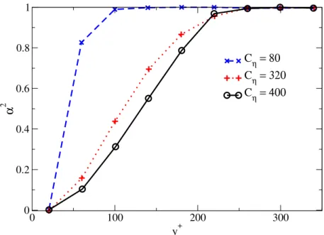
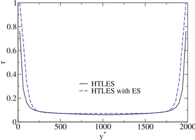
4.3 Channel Flow: Profile of the energy ratio r along the wall-normal direction. 53 4.4 Channel Flow: Profiles ofα2over the altitude for three different values of C_η. 54 4.5 Channel Flow: Illustration of the configuration. . . 55

4.6 Channel Flow: Contours and iso contours (white lines) of the mean axial velocity yielded by HTLES at a streamwise plane cut of the domain. . . 56

(13)

4.7 Channel Flow: Profile of the mean axial velocity over the spanwise direction at centerline yielded by HTLES. . . 57 4.8 Channel Flow: Profiles of the energy ratio r along the wall-normal direction. 58 4.9 Channel Flow: Impact of the elliptic shielding on the dimensionless velocity

profiles for the channel flow Re_τ= 1, 000. . . 59 4.10 Channel Flow: Profile of the streamwise component of the Reynolds stress

tensor: resolved u′xu

′

x

+

(RES), modeledτxx+(SFS) and total T OT = RES +

SF S. . . 60

4.11 Channel Flow: Comparison of the targeted and the observed energy ratio r . 61 4.12 Channel Flow: Comparison of the mean axial velocity along the wall-normal

direction between RANS, LES and HTLES. . . 62

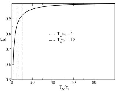
5.1 Channel Flow: Profiles predicted by the recursive HTLES with three different values for the lower bound - Left: k =ks f s_r - Right: energy ratio r . . . 68

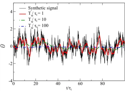
5.2 Transfer function of EWA. . . 71 5.3 Synthetic signal: Kraichnan turbulence spectrum in the frequency domain. 75 5.4 Synthetic signal: Time evolution of the synthetic signal and the filtered

signal for different temporal filter-widths. . . 76 5.5 Synthetic signal: Evolution of ek for different values of the temporal filter

widths. . . 77 5.6 Sinusoidal synthetic signal: Time evolution of the sinusoidal synthetic

sig-nal and the filtered sigsig-nal for different temporal filter widths. . . 78 5.7 Sinusoidal synthetic signal: Phase averaged ek over 100 sine period for

dif-ferent Tw values. . . 79

5.8 Channel Flow: Profiles of the imposed turbulent kinetic energy over the wall-distance. . . 85 5.9 Channel Flow: Profiles of the energy ratio r along the wall-distance

(14)

List of figures 13

5.10 Channel Flow: Profiles of the mean axial velocity U+=Uex

u_τ along the

wall-distance predicted by HTLES for the four different imposed profiles of k. . . . 87 5.11 Channel Flow: Profiles of the mean viscosity ratio along the wall-distance

predicted by HTLES for the four different imposed profiles of k. . . 88 5.12 Channel Flow: Comparison of the profile of an instantaneous temporal

filter-width Twwith the turbulence integral time scales. . . 89

5.13 Channel Flow: Comparison of the profiles of the instantaneous, the time-filtered and the statistical average axial velocities over the wall-distance . . 90 5.14 Channel Flow: Time evolution at a monitoring point located at half height

of the channel of the instantaneous, the time-filtered and the statistically averaged axial velocities. . . 90 5.15 Channel Flow: Comparison of the profiles of the energy ratio r over the

wall-distance yielded by EWA-HTLES and HTLES AVG. . . 91 5.16 Channel Flow: Comparison of the profiles the dimensionless axial velocity

Ux

u_τ over the wall-distance yielded by DNS, EWA-HTLES and HTLES AVG. . . 92

5.17 Steady Flow Rig: Computational domain. . . 93 5.18 Steady Flow Rig: Schematic and geometrical parameters. . . 93 5.19 Steady Flow Rig: Cut-plane of the hexahedral mesh. . . 94 5.20 Steady Flow Rig: Comparison of the dimensionless mean velocity yielded

by LDA measurements, EWA-HTLES and HTLES AVG along l i ne 1. -Left: Axial component. -Right: Radial component. . . 96 5.21 Steady Flow Rig: Comparison of dimensionless RMS velocity yielded by

LDA measurements and EWA-HTLES and HTLES AVG along l i ne 1. -Left: Axial component. -Right: Radial component. . . 96 5.22 Steady Flow Rig: Comparison of the static pressure over the axial distance x

(15)

5.23 Steady Flow Rig: Contours of the mean subfilter to the total turbulent kinetic energy ks f s_k in the central plane yielded by EWA-HTLES. . . 98 5.24 Steady Flow Rig: Instantaneous contours of the velocity magnitude

com-puted in EWA-HTLES at t = 2 s . . . 99 5.25 Steady Flow Rig: Decomposition of the dimensionless RMS velocity along

l i ne 1 into two components, RE S the resolved part and SF S the modeled

part. -Left: axial RMS velocity. -Right: radial RMS velocity. . . 99 5.26 Steady Flow Rig: Decomposition of the dimensionless RMS velocity along

l i ne 2 into two components, RE S the resolved part and SF S the modeled

part. -Left: axial RMS velocity. -Right: radial RMS velocity. . . 100 5.27 Steady Flow Rig: Cut plane of the mean streamlines obtained with RANS,

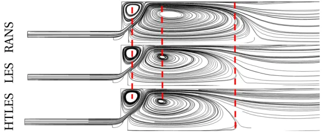
LES and HTLES. . . 101 5.28 Steady Flow Rig: Comparison of dimensionless mean velocity along l i ne

1 yielded by LDA measurements and RANS, HTLES and LES. -Left: axial component. -Right: radial component. . . 101 5.29 Steady Flow Rig: Comparison of dimensionless mean velocity along l i ne

2 yielded by LDA measurements and RANS, HTLES and LES. -Left: axial component. -Right: radial component. . . 102 5.30 Steady Flow Rig: Comparison of dimensionless RMS velocity along l i ne

1 yielded by LDA measurements and RANS, HTLES and LES. - Left: axial component. - Right: radial component. . . 103 5.31 Steady Flow Rig: Comparison of dimensionless RMS axial velocity along

l i ne 2 yielded by LDA measurements and RANS, HTLES and LES. - Left:

axial component. - Right: radial component. . . 104 5.32 Steady Flow Rig: Comparison of the axial profile of static pressure yielded

by the experiment and RANS, HTLES and LES. . . 104

6.1 Compressed Tumble: (a) Sketch of the computational domain. (b) Zoom in on the compression chamber [10]. . . 112 (a) . . . 112

(16)

List of figures 15

(b) . . . 112 6.2 Compressed Tumble: Cut-plane in the symmetry plane of the domain at

BDC. - Left: The whole computational domain. - Right: Zoom in on the compression chamber. . . 114 6.3 Compressed Tumble flow: Cut-plane in the symmetry plane of three meshes.

. . . 114 6.4 Compressed Tumble: Time evolution of the guillotine lift and the piston law.116 6.5 Compressed Tumble: Sketch of the compression chamber and PIV laser

sheet, Figure extracted from [10]. . . 117 6.6 Compressed Tumble: Coordinate system, schematic of the optically

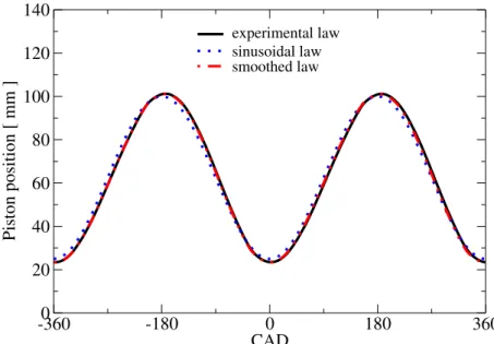
acces-sible area (grey), and the vertical lines over which are extracted the 1D profiles.118 6.7 Compressed Tumble: Time evolution of three piston laws for the

uncom-pressed configuration. . . 120 6.8 Compressed Tumble: -Left: Time evolution of the piston velocity of three

laws for the uncompressed configuration. - Right: Zoom in where the veloc-ity is maximum during the intake. . . 121 6.9 Compressed Tumble: Time evolution of the acceleration of the piston along

the cycle calculated from the smoothed law. . . 122 6.10 Compressed Tumble: Comparison of the time evolution of horizontal

ve-locity at a monitoring point at half height of the channel obtained with three piston laws in RANS. . . 123 6.11 Compressed Tumble: Comparison of the time evolution of the pressure

∆P = (P −Ppl enum)/Ppl enumat a monitoring point at half height of the

chan-nel obtained with three piston laws in RANS. . . 124 6.12 Compressed Tumble: Contours of the velocity magnitude extracted from

PIV and RANS using three different piston laws. . . 124 6.13 Compressed Tumble: Contours and streamlines of the phase-averaged

in-plane velocity in the symmetry in-plane of the compression chamber at 5 instants during the intake. . . 127

(17)

6.14 Compressed Tumble: Vertical 1D profiles of the phase-averaged velocity at 5 instants of the intake. . . 128 6.15 Compressed Tumble: Contours of the mean velocity fluctuations u′xu

′

x in

the symmetry plane at 4 instants of the intake. . . 130 6.16 Compressed Tumble: Contours of the mean velocity fluctuations u′_yu′_yin

the symmetry plane at 4 instants of the intake. . . 131 6.17 Compressed Tumble: Vertical 1D profiles of the mean velocity fluctuations

at 4 instants of the intake. . . 132 6.18 Compressed Tumble: Contours of the integral time scale over T0during

intake. . . 134 6.19 Compressed Tumble: contours of the temporal filter-width Twduring intake.134

6.20 Compressed Tumble: Q+−criterion iso surfaces at 3 in the symmetry plane colored by the instantaneous velocity magnitude at −270 C AD. . . 135 6.21 Compressed Tumble: Contours of the target energy ratio in the symmetry

plane at −270 C AD (5t h cycle). . . 137 6.22 Compressed Tumble: A zoom in on the compression chamber at −270

C AD. - Left: Target energy ratio r . - Right:α2. . . 138

6.23 Compressed Tumble: Contours of r in the symmetry plane at four instants during the intake. . . 139 6.24 Compressed Tumble: Contours of ks f s/k in the symmetry plane at −270

C AD. . . 140

6.25 Compressed Tumble: Decomposition of the velocity fluctuations into two components, the resolved part RES and the modeled part SFS. . . 141 6.26 Compressed Tumble: Comparison of the in-plane phase-averaged velocity

during the intake predicted by HTLES using three meshes. . . 143 6.27 Compressed Tumble: Vertical 1D profiles of the phase-averaged velocity

during the intake predicted by HTLES using three meshes: M1 (finer), M2

(18)

List of figures 17

6.28 Compressed Tumble: contours of the mean velocity fluctuations u′xu

′

x

dur-ing the intake predicted by HTLES usdur-ing three meshes. . . 146 6.29 Compressed Tumble: Contours of the mean velocity fluctuations u′_yu′_y

dur-ing the intake predicted by HTLES usdur-ing three meshes. . . 147 6.30 Compressed Tumble: 1D vertical profiles of the mean velocity fluctuations

during intake predicted by HTLES using three meshes: M1 (finer), M2

(ref-erence) and M3 (coarser). . . 148

6.31 Compressed Tumble: Time evolution of the in-cylinder pressure predicted by RANS, HTLES, and LES versus the experimental data. . . 150 6.32 Compressed Tumble: Contours and streamlines of the phase-averaged

ve-locity during compression. . . 151 6.33 Compressed Tumble: Vertical 1D profiles of the phase-averaged velocity

and the velocity fluctuations during compression. . . 152 6.34 Compressed Tumble: Contours of the phase-averaged viscosity ratio during

compression in the symmetry plane. . . 153 6.35 Compressed Tumble: Time evolution of the number of the upwinded cell

faces in RANS, HTLES and LES simulations. . . 154 6.36 Compressed Tumble: Evolution of the kinetic energy in the symmetry plane

with numbers of averaging cycles at 3 instants of the intake stroke. . . 156 6.37 compressed tumble: Vertical 1D profiles of the first two statistical moments

at −270 C AD. . . 157 6.38 Compressed Tumble: Vertical 1D profiles of the first two statistical moments

at −240 C AD. . . 157 6.39 Compressed Tumble: Vertical 1D profiles of the first two statistical

mo-ments at −180 C AD. . . 158 7.1 Darmstadt Engine: Experimental setup [5]. . . 162 7.2 Darmstadt Engine: Illustration of the two available configurations of the

(19)

7.3 Darmstadt Engine: Computational domain. . . 164 7.4 Darmstadt Engine: A cut of M2 in the intake valve symmetry plane at the

intake with a zoom in on the intake valve region. . . 165 7.5 Darmstadt Engine: Illustration of each mesh in the symmetry plane of the

intake valve at −260 C AD. . . 166 7.6 Darmstadt Engine: Intake and exhaust valve lifts. . . . 167 7.7 Darmstadt Engine: Time evolution of the static pressure at the inlet of the

intake port and at the outlet of the exhaust port. . . 168 7.8 Darmstadt Engine: -Left: Schematic of the cylinder symmetry plane (the

red line). -Right: Contour of the optically accessible cross-section area. . . . 169 7.9 Darmstadt Engine: Schematic of the vertical centerline in the cylinder

sym-metry plane over which are extracted 1D profiles. . . 170 7.10 Darmstadt Engine: Illustration of the coordinate system, and the origin

position, Figure adapted from [15]. . . 170 7.11 Darmstadt Engine: Time evolution of the in-cylinder pressure. . . 171 7.12 Darmstadt Engine: Time evolution of the trapped mass predicted by 3D

simulations and compared to a 1D CFD simulation using GT-Power. . . 173 7.13 Darmstadt Engine: Time evolution of TR predicted by the simulations. . . . 174 7.14 Darmstadt Engine: Time evolution of the standard deviation of TR

pre-dicted by HTLES and LES. . . 175 7.15 Darmstadt Engine: Contours of the energy ratio r at −260 C AD at an

arbi-trary cycle in the symmetry plane of the intake valve. . . 176 7.16 Darmstadt Engine: Q-criterion iso surfaces at 105 1/s2 in the symmetry

plane of the intake valve colored by the instantaneous velocity magnitude at an arbitrary cycle. . . 177 7.17 Darmstadt Engine: Contours of the phase-averaged viscosity ratio on the

(20)

List of figures 19

7.18 Darmstadt Engine: Time evolution of the number of upwinded cell faces in CONVERGE. . . 179 7.19 Darmstadt Engine: Illustration of the flow evolution during intake and

compression, Figure adapted from [55]. . . 180 7.20 Darmstadt Engine: Contours and streamlines of the phase-averaged 2D

velocity magnitude in the cylinder symmetry plane at five instants during intake and compression. . . 181 7.21 Darmstadt Engine: 1D profiles of the phase-averaged velocity along the

vertical centerline in cylinder symmetry line at four different instants. . . 182 7.22 Darmstadt Engine: Contours of uy,R M S in the cylinder symmetry plane

during intake and compression. . . 184 7.23 Darmstadt Engine: Contours of uz,R M S in the cylinder symmetry plane

during intake and compression. . . 185 7.24 Darmstadt Engine: 1D profiles of the RMS velocities over the vertical

cen-terline in the cylinder symmetry plane at four different instants. . . 186 7.25 Darmstadt Engine: Time evolution of the tumble ratio over the crank angle

using M1 (opaque) and M2 (transparent). . . 188 7.26 Darmstadt Engine: Standard deviation of the tumble ratio predicted by LES

and HTLES using M1 (opaque) and M2 (transparent) . . . 189 7.27 Darmstadt Engine: Comparison of the contours and streamlines of the

in-plane phase-averaged velocity in the symmetry plane of the cylinder predicted using two meshes: M1 (coarse) and M2 (reference). . . 190 7.28 Darmstadt Engine: 1D profiles of the phase-averaged velocity along the

vertical centerline in cylinder symmetry line using M1 (opaque) and M2

(transparent) at four different instants. . . 191

7.29 Darmstadt Engine: Comparison of uz,R M S on the tumble plane predicted

(21)

7.30 Darmstadt Engine: Evolution of the kinetic energy along the number of averaged cycles at: - Left: −260 C AD.- Center: −180 C AD.- Right: −90

C AD. . . 194

7.31 Darmstadt Engine: Convergence of the 1D Profiles of the phase averaged velocity and RMS velocity along the vertical centerline at −260 C AD. . . 195 7.32 Darmstadt Engine: Convergence of the 1D Profiles of the phase averaged

velocity and RMS velocity along the vertical centerline at −180 C AD. . . 195 7.33 Darmstadt Engine: Convergence of the 1D Profiles of the phase averaged

(22)

List of tables

4.1 Channel Flow: Main specifications. . . 55 4.2 Channel Flow: Flow rates given by the HTLES with and without the ES. . . . 59 4.3 Channel Flow: Comparison of the flow rates given by RANS, HTLES and LES

to DNS data . . . 62

5.1 Sinusoidal synthetic signal: Main dimensionless specifications. . . 78 5.2 Coefficients of the HTLES approach. . . 82 5.3 Stationary configurations: Set of the numerical parameters used for RANS,

HTLES and LES. . . 84 5.4 Stationary configurations: Turbulence models used for RANS, HTLES and

LES. . . 84 5.5 Channel Flow: Flow rates yielded by DNS and HTLES. . . 92 5.6 Steady Flow Rig: Main specifications. . . 94 5.7 Steady Flow Rig: Comparison of the pressure drop given by the experiment

and RANS, HTLES and LES. . . 105

6.1 Compressed Tumble: Dimensions of the compressed tumble. . . 112 6.2 Compressed Tumble: Grid resolutions of M 1, M 2, and M 3 in each region. . 114 6.3 Compressed Tumble: Numerical parameters. . . 115

(23)

6.4 Compressed Tumble: Turbulence models used for RANS, HTLES and LES. . 115 6.5 Compressed Tumble: x−coordinate of the 1D vertical profiles. . . 118 6.6 Compressed Tumble: Specifications of the sinusoidal and the experimental

piston motion laws. . . 120

7.1 Darmstadt Engine: Main specifications. . . 163 7.2 Darmstadt Engine: Grid resolution for each region and each phase of the

four-stroke cycle for Mesh 2. . . 165 7.3 Darmstadt Engine: Numerical parameters. . . 166 7.4 Darmstadt Engine: Temperatures at the wall boundaries. . . 168 7.5 Darmstadt Engine: Experimental and predicted peak pressure at TDC. . . . 171

(24)

Chapter 1 Introduction

1.1 Environmental context

The fight against global warming and the reduction of the atmospheric pollution are mean-ingful environmental concerns in our industrial societies. Greenhouse gas emissions from the transportation sector increased by 8% between 1990 and 2015, representing 23% of overall greenhouse gas emissions [27]. Following civil society and environmental organi-zation pressures, CO2emission targets for vehicle fleets set by the European commission

are more and more stringent. These restrictions force the automobile industry to develop less polluting vehicles.

(25)

Fig. 1.1 Evolution of CO2emissions for passenger cars by fuel types (source: European

Environ-ment Agency).

As shown in Figure 1.1, CO2emissions for Petrol (Gasoline), Diesel, and Alternative

Fuel Vehicles (AFV) have been continuously decreasing since 2000 and the target for 2020 is very challenging, with a target CO2emission of 95 g per km [27].

In this context, electric vehicles appear as a promising alternative to thermal engine vehicles. However, despite its growing trend, the market share of electric vehicles only amounted to 2.6% of global car sales in 2019. Therefore, Internal Combustion Engines (ICE) will still be leading the market shares in the next years [98]. This is particularly true for hybrid electric vehicles that combine ICE with an electric propulsion system, and freight transport, for which ICE remains the more suitable propulsion solution.

1.2 Spark-Ignition (SI) engines

A growing number of vehciles worldwide are equipped with SI engines. These engines operate according to the four-stroke Otto cycle as illustrated in Figure 1.2:

(26)

1.2 Spark-Ignition (SI) engines 3

Intake

Compression

Expansion

Exhaust

Fig. 1.2 The four-stroke cycle [36].

1. The intake stroke: during this phase, the piston moves down and the intake valves open. Air is then drawn into the cylinder through the intake valves and the fuel is sprayed through a fuel injector.

2. The compression stroke: the piston moves towards TDC and all the valves close, resulting in the compression of the air-fuel mixture in the cylinder.

3. The expansion stroke: a spark discharge ignites the air-fuel mixture. The chemical energy of the fuel is released and converted into heat. The burnt gasses expand, pushing down the piston during the expansion stroke.

4. The exhaust stroke: the exhaust valves open, and as the piston moves toward TDC, the exhaust gas moves out from the cylinder as the piston moves up.

Car manufacturers dedicated important efforts to reduce CO2emissions by increasing

engine efficiency in different ways, such as:

• The reduction of the heat losses at the outer walls of the combustion chamber [64]. • The reduction of the combustion duration by acting on the in-cylinder

aerodynam-ics.

• An optimized spark timing in order to release energy at the proper time in the cycle. This also depends on the in-cylinder flow, as the latter plays a major role to prepare the air-fuel mixture.

Modern SI engines include technologies that implement such strategies. In this context, special attention is dedicated to the in-cylinder flow as it was shown that it can promote

(27)

rapid and stable combustion in SI engines [51]. Indeed, most modern SI engines are designed in such a way that the air sucked into the combustion chamber forms a large-scale rotational motion around the axis perpendicular to the cylinder axis. This motion is called the tumble motion. As a consequence of its compression, it breaks down into small turbulent scales shortly before the combustion. The increased turbulence allows to obtain a better air-fuel mixture and higher combustion speed which enhances the engine efficiency.

Nonetheless, modern SI engines suffer from a limiting issue called Cycle-to-Cycle Variability (CCV), which manifests by substantial variations in in-cylinder conditions of the engine at a fixed operating point. The difficulty is that several engine parameters (e.g. spark timing and injected fuel mass) are set based on averaged data. Using these parameters in an engine with high CCV levels can lead to combustion efficiencies and pollutant levels that are far from the nominal values if in-cylinder conditions were perfectly repeatable.

1.3 Roles of CFD in the SI engine development process

Industrials dedicate continuous effort to understand the occurrence of CCV, and to imple-ment solutions to avoid them. Computational Fluid Dynamics (CFD) tools have become fundamental tools used today in the ICE development process. They can support the design of engine parts as well as provide a better understanding of the occurrence of CCV. Turbulent flows encountered in ICE are wall-bounded, characterized by Reynolds numbers between 10, 000 and 30, 000 [115], and comprise multi-physics processes such as combustion, multiphase flow, spray formation, and heat transfer.

Simulating all the scales of motion using Direct Numerical Simulation (DNS) remains far beyond computers’ capabilities, both at present and in the near future. Therefore, turbulence modeling approaches are used to reduce the computational simulation cost.

Reynolds-Averaged Navier Stokes (RANS) is the most widely used approach in the industry, mainly because of its low computational cost. Nonetheless, this approach uses statistical averaging, which only provides phase averages of the flow quantities making CCV assessment difficult [115, 117]. Furthermore, several studies highlighted its limited accuracy in complex flows involving shear flows and flow separation that are encountered in ICE flows [24]. Alternatively, Large-Eddy Simulation (LES), is another

(28)

1.4 Objectives of the present thesis 5

well-known approach, has an improved ability to predict unsteady phenomena such as CCV occurrences [114, 115]. LES uses spatial filtering to identify large turbulent scales and resolve them, while the unresolved small scales are modeled. LES requires that the grid size be sufficiently fine to solve a large enough part of the turbulent energy, inducing a high computational cost, especially near the wall where turbulent structures are small [7]. Wall modeling strategies reduce the computational cost of LES at the walls by modeling the boundary layers using wall-functions. Apart from the gain in computational cost, applications of wall-modeled LES (WMLES) in ICE flows have shown limited accuracy for the wall friction assessment [79, 96, 115].

An alternative to WMLES consists in combining RANS and LES models in the same computational domain in a so-called hybrid RANS/LES approach. Such approaches aim at reducing the computational cost of the simulations by using RANS at the walls and where a statistical description of the flow is sufficient. Furthermore, it was shown that some of these models could further decrease the simulation cost by using relatively coarser meshes than for LES [24, 26, 115, 124].

1.4 Objectives of the present thesis

Despite the development of different hybrid methods, few of them were applied to ICE flows. In this context, the present work aims to develop a hybrid RANS/LES model for ICE flows based on a theoretical framework capable of meeting the following requirements:

• The developed model must be compatible with ICE cyclic flows with moving wall boundaries and time-varying boundary conditions.

• It should be able to switch automatically between RANS and LES in order to be easily used in non-stationary flows.

• It should be able to operate in RANS at the walls and where the mesh is too coarse for LES.

• The model should be able to reduce the computational cost compared to LES by resolving turbulent scales in relatively coarse meshes.

Among the existing hybrid models, the Hybrid Temporal RANS/LES (HTLES) [80, 81, 129] approach was selected as the starting model for its theoretical framework and

(29)

its compliance with some of the requirements mentioned above. The model uses the multiscale approach [28, 29, 34, 118, 119] in the time domain to define the modeled scales, which offers a well-defined framework for the RANS-LES transition in stationary flows [19, 38]. Nevertheless, this model is recent, it is only compatible with stationary flows, and it has not been extensively used in complex configurations.

The present work aims at extending HTLES to ICE engine flows. First, HTLES was implemented in the Converge CFD code [112], and validated in stationary configurations. Particular attention was paid to the ability of HTLES to switch to RANS at the walls. It was found that the model has a grid-dependent behavior near the wall and did not ensure RANS at the walls. A shielding function that ensures RANS at the walls was developed for this purpose. HTLES was then extended to cyclic ICE flows by adapting the method for evaluating the mean quantities used in the model. The developed model was validated in stationary configurations. The results of the simulations were compared with the reference data and with RANS and LES. Finally, it was applied to two optical engines: the compressed tumble engine and the Darmstadt engine. The predictions of mean and rms velocities, as well as the ability of the model to resolve CCV were assessed and the results were compared with experimental findings, and with RANS and LES.

1.5 Outline of the manuscript

Part I introduces the governing flow equations and the main approaches of turbulence

modeling

• Chapter 2 provides the Navier Stokes equations and the main characteristics of turbulent flows.

• Chapter 3 introduces the different modeling approaches of turbulence. It also comprises a literature review on the studies that applied RANS, LES and hybrid RANS/LES to ICE flows.

Part II is dedicated to the theoretical developments of the Hybrid Temporal RANS/LES

(HTLES) model for cyclic ICE flows and its validation in stationary configurations: • Chapter 4 presents the theoretical framework of the original HTLES model, and

details its implementation in the Converge CFD code. An elliptic shielding was developed to ensure that HTLES operates in RANS at the walls. Then a validation in

(30)

1.5 Outline of the manuscript 7

a channel flow is provided. The main findings of this Chapter were published (see Appendix 8.2):

Development and validation of a hybrid temporal LES model in the perspective of applications to internal combustion engines.

Afailal A. H., Galpin J., Velghe A. and Manceau R.

Oil Gas Sci. Technol. – Rev. IFP Energies nouvelles, 74 (2019) 56 .

• Chapter 5 is dedicated to the extension of HTLES to cyclic ICE flows. It first discusses

different approaches that have been explored in this work , before detailing the approach that was retained and developed. Finally, the developed model is validated in two stationary configurations: a channel flow at Re_τ= 1, 000 [77] and a steady flow rig [127], which represents an engine-like configuration. For each configuration, the simulation results are analyzed and compared with the reference data and with RANS and LES.

Part III provides the results of the developed model in two non-reacting engine flows. For

each engine, the simulation results were examined on different meshes, and compared with PIV findings, and with RANS and LES.

• Chapter 6 presents the results of HTLES in the compressed tumble engine. This configuration consists of a simplified square engine that reproduces the generation and the tumble motion breakdown.

• Chapter 7 exposes the results of HTLES in the Darmstadt engine. This configuration is similar to a SI engine.

(31)

(32)

Part I

(33)

(34)

Chapter 2 Theoretical aspects of turbulent flows

This Chapter gives the governing equations and the main characteristics of compressible turbulent gas flows, which constitute the context of this work. It starts by providing the Navier-Stokes equations, before giving the main characteristics of turbulent flows.

2.1 Governing equations

The mathematical formulation of any Newtonian compressible flow expresses using Navier-Stokes equations − the continuity, momentum and energy equations :

         ∂ ∂tρ +∂x∂j(ρUj) = 0 ∂ ∂t(ρUi) +_∂x∂_j(ρUiUj) = −_∂x∂_ip +_∂x∂_jσi j ∂ ∂t(ρE) +∂x∂j(ρUjE ) = − ∂ ∂xj(Ui(pδi j− σi j) + qj) (2.1)

whereρ denotes the density, and Ui is the it hcomponent of the velocity. p is the static

pressure.σi j= 2µ(Si j−1₃Skkδi j) is the stress tensor, with Si j=1₂(∂U_∂x_ji+∂U_∂x_ij) is the strain

rate tensor. E is the total energy, and q is the heat flux.

The Redlich-Kwong equation of state [109] is used for gases to couple the density, pressure and temperature:

p = RT

Vm− b

−p a

T Vm(Vm+ b)

(35)

where R = 8.314 J.mol−1.K−1is the gas constant. T is the temperature. Vmis the molar

volume. a = 0.42748 ×R2Tc5/2

Pc and b = 0.08664 ×

RTc

Pc , with Tc and Pc are the temperature and the pressure at the critical point.

One of the non-dimensional numbers used to characterize the flows is the Reynolds number [110]:

Re =U L

ν (2.3)

The Reynolds number expresses the ratio of the inertial forces to the viscous forces. U and L denote the characteristic velocity and length scale of the flow, respectively. A high Reynolds number means that the inertial forces overweight the viscous forces, possibly giving rise to chaotic flow motions, i.e, turbulence.

2.2 Main characteristics of turbulence

In order to understand turbulence processes, Richardson [113] introduced the energy cascade concept. According to this theory, turbulence is a composition of eddies of different sizes. The kinetic energy enters the turbulence at the largest eddies. This energy is then transferred from the large eddies to the small ones by inviscid processes. It goes on until reaching the smallest scales, where the turbulent energy is dissipated into heat by viscous forces. Kolmogorov completed this theory by quantifying the length, time and velocity scales to describe the smallest eddies:

• Kolmogorov length scaleη = (ν_ε3)1/4 • Kolmogorov time scaleτ_η= (ν_ε)12 • Kolmogorov velocity u_η= (νε)1/4

whereν is the kinematic viscosity of the fluid and ε = ν∂u ′

i

∂xk

∂u′i

∂xk is the turbulent dissipation rate. The Reynolds averaging operator and the fluctuating velocities u′_i are introduced in Section 3.2.1.

In-depth analysis of the turbulence process can be achieved through the Fourier transformation of the turbulent energy, which expresses as:

E (κ,t) =

Z Z Z +∞

−∞

1

(36)

2.2 Main characteristics of turbulence 13

whereδ is the Dirac distribution, κ is the wave number related to the length scale of the eddies l as:κ = 2π/l and φi jis,

φi j(κ,t) = 1 (2π)3 Z Z Z _+∞ −∞ e−i κrRi j(x, r, t )d r, (2.5)

where Ri j is the two-point correlation,

Ri j(x, r, t ) = u′_i(x, t )u′_j(x + dr, t) . (2.6)

Fig. 2.1 Energy cascade of homogeneous isotropic turbulence [91].

Figure 2.1 shows the energy cascade profile in the framework of Homogeneous Isotropic Turbulence (HIT). The energy spectrum can be divided in three regions [63]:

• Energy-containing range: consists of the largest eddies where the turbulence energy is generated by the mean flow.

• Inertial sub range: it this range the turbulent energy is transferred from large to small eddies. The turbulence is generally assumed to be isotropic in the inertial sub range. The energy in this range follows the Kolmogorov law:

E (κ) = C_κε2/3κ−5/3 (2.7)

(37)

• Dissipation range: the dissipation takes place within the smallest scales where viscous effects become preponderant leading to the dissipation of the turbulent kinetic energy into heat.

These analyses give an overview of turbulence mechanisms and have played an important role on turbulence modeling.

(38)

Chapter 3 Modeling approaches of turbulence

Direct Numerical Simulation (DNS) is the simplest approach to simulate turbulent flows since the Navier-Stokes equations are directly discretized and solved numerically [116]. However, such an approach is not possible for ICE flows that are turbulent and contain a wide range of length and time scales, which requires an unaffordable computational cost for their resolution [104, 115, 116, 122]. Instead of resolving all scales of motion, the computational cost associated with the simulation of turbulent flows can be reduced by resolving only some specific scales of the flow and model the unresolved scales using a physical model.

3.1 Scale separation operator

The scale separation operatorF aims to distinct the resolved and the unresolved tur-bulent scales. By applying this operator to any variable of the problem f the following decomposition is obtained:

f = F (f ) + f′, (3.1)

where f = F (f ) and f′are the resolved and unresolved turbulent scales, respectively. The scale separation operator admits two different natures, depending of the approach of describing the flow:

• Statistical approach (RANS) which consists of a statistical description of the flow where only averaged flow quantities are resolved. In this approach, F relies on

(39)

statistical averaging: f = 1 N N X i =1 fi, (3.2)

where fi is the it hrealization of the flow and N is the number of the included

realiza-tions. N must be sufficiently large enough to remove all the turbulent fluctuations from f .

• Filtering approach (LES) which consists in separating the large energy-containing eddies from the small scales responsible for the energy dissipation. The general form ofF consists of the Kampe de Fériet and Betchov spatio-temporal low-pass filter [30]: F ( f )(x, t ) = Z D Z t −∞ G(x, x′, t , t′) f (x′, t′)d x′d t′ (3.3)

where G is the filter’s kernel

The set of equations obtained after applying the scale separation operator to the Navier-Stokes expresses as [116]:    ∂ ∂tρ +∂x∂j(ρUj) = −A1, j ∂

∂t(ρUi) +_∂x∂_j(Uj ρUi) = −_∂x∂_ip +_∂x∂_jσi j− (A2,i+ A3,i+ A4,i)

(3.4)

Ai are the residual terms: A1, A3and A4are relative to the commutation errors of the

scale separation operator and the spatial and temporal partial derivatives, while A2is

associated with the non-linearity of the convective term. It corresponds to the spatial derivative of the unresolved stress tensor. The residual terms express as [116]:

           A1,i = (ρ[F, ∇.]U; ei)

A2,i = (ρ∇.[F, B](U, U); ei)

A3,i = (ρ([F, ∇.]B(U, U) + [F , ∇]p + ν[F , ∇2]U); ei)

A4,i = (ρ[F,_∂t∂]U; ei)

(3.5)

with [ f , g ]h = f ◦ g (h) − g ◦ f (h) is the commutator operator, B is the cross product, (f ; g ) is the scalar product, (ei)i =1,3is the unit vector in the it hcoordinate direction and U is the

(40)

3.2 Reynolds Average Navier-Stokes (RANS) 17

3.2 Reynolds Average Navier-Stokes (RANS)

3.2.1 Reynolds decomposition

According to the Reynolds decomposition, any variable of the flow f writes as:

f = f + f′ (3.6)

where f is the statistical average of f , and f′are the turbulent fluctuations. In stationary flows, Monin and Yaglom [92] demonstrated that the statistical average can be replaced by a time average: f = lim ∆T →+∞ 1 ∆T Z ∆T 0 f (τ)dτ (3.7)

Contrary to stationary flows, the statistical average in cyclic flows (as ICE flows) is time varying and corresponds to a phase average [52]:

f (t ) = 1 N N X i =1 f (t + i T0) (3.8)

where t is the instant, N is the number of the included cycles to compute the phase average and T0is the cycle period.

The averaging operator has the following properties: Constant conservation a = a Linearity a f = a f f + g = f + g Commutativity [_∂ξ∂, (.)] = 0, ξ = t,xi Projectivity f g = f g Idempotence f = f f′ = 0

where a is a constant, and f and g are functions depending on time and space. The Reynolds operator is idempotent and commutes with space and time operators. Therefore the residual terms Aireduce to:

(41)

(

A1,i = A3,i = A4,i = 0

A2,i = (∇.τ, ei)

(3.9)

τi j is the Reynolds stress tensor:

τi j= u

′

iu

′

j (3.10)

In compressible flows, turbulent fluctuations can result in significant fluctuations in density, i.e.,ρ′̸= 0. Using the Reynolds operator in this situation leads to complex averaged equations. In this situation, we use the Favre average [39]:

e

f =ρ f

ρ . (3.11)

The decomposition expresses as:

f = ef + f", (3.12)

where f"is the unresolved part of f .

Despite the density average being not idempotent, f"_{̸= 0, we use to derive averaged}

Navier-Stokes equations as it leads to much simpler equation than the ones obtained with the Reynolds average.

The set of equations given by the averaging operator is called Reynolds-Averaged Navier-Stokes (RANS) equations [39]:

         ∂ ∂tρ +∂x∂j(ρUej) = 0 ∂ ∂t(ρUei) +_∂x∂ j(ρUejUei) = − ∂ ∂xip + ∂ ∂xjσi j− ∂ ∂xjρτi j ∂ ∂t(ρE ) +e _∂x∂ j(ρUejE )e = − ∂ ∂xj(Uej+U "_{p + ρU}" jE −Uiσi j) +qej) (3.13)

whereσi j= 2µ( eSi j−1₃Se_kkδ_{i j}) is the viscous stress strain tensor withSe_{i j}=1

2(

∂Uei

∂xj +

∂Uej

∂xi ) the strain rate tensor, andτi j= u"_iu"_j the turbulent stress tensor.

3.2.2 Overview of RANS models

The Reynolds stress tensor represents all the turbulent fluctuations. These fluctuations are not resolved in RANS and need to be modeled.

(42)

3.2 Reynolds Average Navier-Stokes (RANS) 19

The first modeling method is called Reynolds Stress Model (RSM). It consists in solving a transport equation for each Reynolds stress component. This approach is rarely em-ployed in the automotive industry because of its complexity and its computational cost, since at least the six transport equations related to the six components ofτi j needs to be

solved. The second modeling method uses the turbulent-viscosity concept introduced by Boussinesq, in which the Reynolds stress tensor writes according to the Boussinesq relation (Boussinesq, 1877):

− τi j+

2

3kδi j= 2νtSei j (3.14)

where k is turbulent kinetic energy andνt is the turbulent viscosity. This approach is

called the linear Eddy-Viscosity modeling (EVM) strategy. It reduces the resolution of the six-components of the Reynolds stress tensor to the assessment of a single scalar called turbulent viscosityνt . This approximation is inspired from the Newton law for the

molecular agitation stress [110] and is a retranscription of this law at a macroscopic scale. This remains a simple approximation of the physics of turbulence and the Boussinesq hypothesis is still the subject of many questions in terms of validation for simple-shear flows, swirling flows or flows with strong anisotropy [104]. Despite the limits of this approach, viscosity modeling is widely used in engineering applications. The eddy-viscosity approximation was studied by Prandtl who was one of the first to introduce an algebraic model of the turbulent viscosity based on the mixing length concept [105]. From a dimensional analysis, the turbulent viscosity can be interpreted as the product of a fluctuating velocity and a characteristic scale:

νt= u"l , (3.15)

In RANS, these quantities are based on integral scales of the turbulence. For example, in the two-equation models, one transport equation solves the turbulent kinetic energy k which is related to the fluctuating velocity u"≈pk and another equation is dedicated to an

additional turbulent quantity that allows to define the length or time scales of turbulence. In the k − ε model, the turbulent dissipation rate ε allows to compute the turbulent length scale l ≈ k3/2_ε . This model was generalized by Jones & Launder [74] for wall-bounded flows by introducing a damping function that provides an appropriate turbulent viscosity in the near wall regions. Wilcox proposed to resolve the turbulence frequencyω in the two-equation k − ω model [132]. The model enhances the near-wall modeling without any modification of the equations unlike the k − ε model. These two-equation models have been applied successfully in various applications. However both models suffer from a lack of versatility in certain configurations. For instance, the k − ε model showed a

(43)

lack of sensitivity to adverse pressure-gradients, which delays or prevents separation [62]. Furthermore, this model has some numerical issues in full-wall integration due to the non-linear damping functions introduced near-wall [74], as well as stiff boundary conditions

forε at no-slip surfaces. In contrast, the k −ω model performs better than the k −ε model

in situations with adverse-pressure gradients [89], and alleviates the numerical stability issues encountered in the k −ε model thanks to the simple formulation of ω in the viscous sub layer [132]. Therefore, the main drawback of the k −ω model is the strong dependency of the results on the free stream value ofω as pointed in [89]. It has been shown that the magnitude of the eddy-viscosity can change by more than 100% by changing the free stream values ofω. The shear-stress transport (SST) model [88] reduces this problem by using a zonal approach that switches between k −ω and k −ε where they perform the best. This model is identical to the original k − ω model in the inner 50% of the boundary layer and switches to the k − ε model in the free stream. The model uses the change of variable

ε = Cµkω to transform the ε-equation into a ω-equation so that one homogeneous set of

equations based on k andω is obtained. The switch between the k − ω model and the

k − ε is operated using a blending function F1that depends on the distance from walls.

The set of equations of the k − ω SST model is given in Appendix 8.2

3.2.3 Near-wall flow modeling

Wall boundaries give rise to boundary layers where the velocity varies from no-slip condi-tion at wall to its free stream value. In these regions, the viscous effects play important role and the wall-distance is expressed in dimensionless wall-distance y+= u_ντy. The dimensionless wall-distance can be seen as the ratio of the distance from the wall y to the viscous length scaleδ_ν.

From a computational point of view, the resolution of the turbulence in the near-wall region requires high computational resources and is seldom affordable for industrial purposes. Instead of resolving the boundary layers, it is possible to use a wall modeling approach in which the effects close to the walls are taken into account through a model. The next Sections introduce the characteristics of turbulent flows near the wall, then propose a wall-function model. The resolution of the boundary layer in RANS requires a fine grid such as y+< 2 in the whole computational domain [86]. Wall modeling allows to reduce significantly the computational cost. The mesh in the boundary layer can be coarsen in such a way that the condition y+< 2 is no more necessary. The effects of the unresolved near wall physics is modeled by a wall-function. Wall-functions are derived

(44)

3.3 Large-Eddy Simulation (LES) 21

from the law-of-the-wall which has been established in the framework of a channel-flow in which strong assumptions have been considered. These assumptions are not verified in general flows. However, in practice the resolution of the boundary layer is challenging and the use wall functions is often preferable.

Wall-functions are in practice applied to compute the shear stress for the momentum equations at the walls as:

τw= ρu_τ∗2

Ut ,p

U∗_p (3.16)

where p indicates the cell adjacent to the wall, Ut ,pis the tangential mean velocity and u∗_τ

is the nominal shear velocity defined as:

u_τ∗= C_µ3/4 q

kp (3.17)

U∗_pis given by the law-of-the wall [104]:

U∗_p= u∗_τ(1

κl n(y∗p) + B) (3.18)

whereκ = 0.41 and B = 5.2. y∗_pcorresponds to:

y_p∗=ypu

∗

τ

ν (3.19)

This formulation is applied for y_p∗≥ 11.3, which corresponds to the intersection of the log law and the linear law U+= y+. For y_p∗< 11.3, the nominal mean velocity is calculated from the viscous sublayer profile:

U∗_p= yp∗u∗τ (3.20)

This simple switch from Equation 3.18 to 3.20 at y_p∗= 11.3 is motivated by the lack of theoretical results in the buffer layer.

3.3 Large-Eddy Simulation (LES)

In Section 2.2, the energy cascade theory showed that the turbulent process can be consid-ered as a composition of eddies of different sizes. LES uses a low-pass filter that separates the large eddies from the small ones. The large eddies are resolved by the simulation while

(45)

the effects of the small eddies which are below the filter cutoff are taken into account by a mathematical model.

3.3.1 Filtered Navier-Stokes equations

In LES, the scale separation operatorF corresponds to a convolution filter [104]: F (f )(x,t) =

Z

f (x − θ, t)G∆(θ,x)dθ , (3.21)

whereF (f ) = f are the filtered variables, which contains only the contribution of the large eddies. The integration is performed over the entire flow domain, and G_∆is the filter function which satisfies the normalization condition:

Z

G_∆(θ,x)dθ = 1 . (3.22)

In simulations, the filter is not explicitly applied to the variables, but results from the combined influence of the subgrid viscosity and the numerical viscosity.

Spatial convolution filters are not idempotent, such that: (

f ̸= f

f′ ̸= 0 . (3.23)

To obtain the governing equations of the filtered scales, a convolution filter is applied to Navier-Stokes equations (see Equation (3.4)). The convolution filter commutes with time and space operators only if the filter-width is homogeneous in the entire flow domain. In practice, the filter-width is not strictly homogeneous in the entire computational domain. Therefore, when moving the derivative out of the integral, the commutation error is proportional to O(∆x2_{) [42]. This order of accuracy is close to that of numerical schemes}

used in industrial applications. Hence, the commutativity can be assumed within this framework, which leads to the simplification of the residual terms:

(

A1,i = A3,i = A4,i = 0

A2,i = (∇.ρτsg s, ei)

(3.24)

(46)

3.3 Large-Eddy Simulation (LES) 23

Thus, in the compressible regime, the filtered Navier-Stokes equations expresses as:

   ∂ ∂tρ +∂x∂j(ρUej) = 0 ∂ ∂t(ρUei) +_∂x∂ j(ρUejUei) = − ∂ ∂xip + ∂ ∂xjσi j− ∂ ∂xjρ τsg s,i j (3.25)

whereσi j= 2µ( eSi j−1₃Se_kkδ_{i j}) is the filtered viscous stress strain tensor withSe_{i j}=1₂(∂

e

Ui

∂xj +

∂Uej

∂xi) the filtered strain rate tensor, and:

τsg s,i j = UiUj− fUiUf_j (3.26)

The subgrid stress tensor represents all the interactions between the filtered and subgrid scales [39]:                  τsg s,i j = Li j+Ci j+ Ri j Li j= U_e_iU_e_j− eU_iU_e_j Ci j= u"_ifU + _j u"_jfU_i Ri j= u" iu " j (3.27)

• the Leonard tensor Li j contains only the filtered velocities. It represents the

interac-tion among the large scales.

• the cross tensor Ci jrepresents the interaction between the filtered and the subgrid

scales.

• the Reynolds stress tensor Ri j represents the interaction between the subgrid scales.

Even if onlyUiUj is unknown inτsg s, the subgrid stress tensor is entirely modeled. There are two possible ways to modelτsg s:

• Structural models that assess the subgrid stress without introducing the subgrid viscosity concept [103].

• Functional models that assess the residual stress using the Boussinesq hypothesis:

τi j ,sg s= −2νsg sSe_{i j}+ 1

3τkk,sg sδi j , (3.28) whereνsg sis the subgrid viscosity.

(47)

Many subgrid models are generally developed using the Kolmogorov assumption, and assumes that the subgrid production and the dissipation rate are equal. This requires to be well in the inertial sub-region of the turbulence energy spectrum.

Different mesh resolution criteria have been proposed for LES. For example, Pope [104] recommended that the filter-width should cover at least 80% of the resolved fraction of the energy spectrum. If the filter-width is close to the energy containing area, the hypothesis of equilibrium of the sugbrid scales is not necessarily verified and thus the dissipation rate can be different from the subgrid turbulent production, which results in a misestimate of the subgrid viscosity [104].

3.3.2 Temporal LES (TLES)

While LES has been mostly used with spatial filtering, some authors attempted to replace it by a temporal filter, leading to the so-called Temporal LES (TLES). The reasons that motivated this choice include the following [19]:

• In contrast with spatial filters, the width of the temporal filter can be taken uniform in the domain, which ensures the commutativity with spatial derivatives [42]. How-ever, this is of limited interest, since the purpose of LES/TLES is to adapt the filter width to local flow conditions.

• Dakhoul and Bedford [23] showed that, unlike temporal filtering, spatial filtering is inconsistent in flows that comprise time-dependent point sources.

• By using temporal filtering, the linkage with RANS solutions can be properly defined in stationary flows. Indeed, the statistical average is the limit of the temporal filter when the temporal filter width goes to infinity [38]. This property motivates the use of temporal filters in the following chapters.

The finite time filtering for turbulence was originally proposed by Boussinesq [107]. Few works were dedicated to the time filtering of turbulence. Dakhoul and Bedford [23] and Aldama [2] proposed spatio-temporal filtering while Meneveau et al. [85] developed a Lagrangian time-domain filter for LES. For its part, Pruett [19] proposed the temporal LES using temporal filtering in the Eulerian time domain[106].

In what follows, we focus on Pruett’s work on the development of the TLES concept. The scale separation operator corresponds to a causal temporal filter in the Eulerian-time

(48)

3.3 Large-Eddy Simulation (LES) 25 domain [19]: F (f )(x,t) = Z t −∞ f (τ,x)G(τ − t,Tw)dτ , (3.29)

where G is the kernel that must satisfy:

G(t , Tw) = 1 Tw g ( t Tw ) , (3.30)

where Twis the temporal filter width and g is any integrable function such that:

(

g (0) = 1

lim_{t →−∞}g (t ) = 0 (3.31)

The Temporally Filtered Navier-Stokes Equations (TFNS) are formally identical to the spatially filtered Navier-Stokes Equations (3.25). The difference lies in the interpretation of the filtered fields, which correspond in TLES to temporally filtered quantities rather than spatially filtered quantities as in LES.

The residual stress, also called the subfilter stress in the temporal framework, is for-mally identical to the one obtained in LES:

τSF S,i j = UiUj− fUiUfj (3.32)

Another interesting feature of filtering in the time-domain is that when Twtends to +∞ in

stationary flows,τSF Sasymptotically approaches the RANS Reynolds stress [106].

As far as we know, only the Temporal Approximate Deconvolution Model (TADM) exist in the literature to model the subfilter stresses [106]. Indeed, in stationary flows, the statistical quantities are independent of time and the statistical average is equivalent to the long-time average. Since temporal filtered quantities tend to the long-time averaged quantities when the filter width Tw goes to infinity, the TLES equations tend to the RANS

equations.

3.3.3 Limitations of LES in industrial applications

The high computational cost of LES remains the main factor limiting its widespread use. Indeed, in wall-bounded flows, the grid requirement of LES scales with the friction Reynolds number as Re_τ2, which is today unfeasible for most industrial applications [104].

(49)

The high computational cost of LES is essentially related to the resolution of the boundary layers:

• the turbulent scales in the boundary layers are rather small. For example, Davidson [24] recommends a grid resolution expressed in wall-units of: y+= 1 for the wall-normal direction, x+= 100 for the streamwise direction and z+= 30 for the spanwise direction.

• LES requires small CFL values to reduce error due to the temporal discretization. Thus, the grid resolution requirement near the wall induces small time-steps, which increases the overall turnaround time of the simulation.

Similarly to RANS, Wall-Modeled LES (WMLES) uses wall-functions to reduce the com-putational cost of the simulation. The grid requirement in WMLES increases weakly as

l n(Re_τ) instead of Re_τ2for wall-resolved LES. Despite the continuous efforts that have

been dedicated to develop wall-models, developing sufficiently general model is still a challenge [18, 20, 59, 101]. These models are generally adaptations of RANS wall-functions or 1D simplifications of RANS models which have shown limited accuracy in the prediction of the wall friction [60, 79, 96]. This is potentially due to the inconsistency between LES fields, which relies on the spatial filtering and wall functions that provide statistical averaged quantities rather compatible with the RANS framework.

Next Section introduces hybrid RANS/LES models that present a promising alternative to WMLES.

3.4 Hybrid RANS/LES turbulence models

3.4.1 Concept

Despite the numerous studies that outline the advantages of LES over RANS modeling [25, 122, 123] and the relevance of LES to simulate ICE flows [115], Section 3.3.3 showed that the stringent mesh requirement of LES still limits its widespread use in the industry. The hybrid RANS/LES concept was proposed within this context. Hybrid models decrease the computational cost of LES by using RANS where LES is too expensive or where a statistical description of the flow is sufficient. This is made possible thanks to the RANS and LES equations which are formally identical, even if they represent variables of different

(50)

3.4 Hybrid RANS/LES turbulence models 27

physical natures (statistically averaged and spatially filtered quantities, respectively). In the framework of eddy viscosity models, the Boussinesq relation is applicable for both approaches to model the residual stress:

τi j= −2νtSe_{i j}+ 1

3τkkδi j . (3.33)

whereνt can be expressed from a dimensional interpretation as:

νt= u"l . (3.34)

where u"is a velocity scale and l is a length scale.

The difference between RANS and LES lies in the interpretation ofνt:

• in RANS, u"and l are computed from integral scales of turbulence in such a way thatνt models the effects of all the turbulent fluctuations.

• in LES, u"and l are based on the local grid step so thatνt models the effects of the

subgrid scales upon the filtered scales.

Hybrid RANS/LES methods aim to propose turbulence models that are able to switch between the two approaches. Many efforts have been dedicated to the development of hybrid methods during the last decades. They resulted in the development of a wide variety of models which differ, first by the way how the transition between RANS and LES is operated and second by the theoretical background.

3.4.2 Classification

Sagaut et al. proposed the following classification of hybrid methods [116]:

• Zonal hybrid methods rely on a discontinuous treatment at the RANS-LES interface. The RANS and LES regions are predefined by the user, and RANS and LES models are used in each region. The LES content has to be explicitly reconstructed at the inlet of a LES region to take into account the lack of resolved fluctuations in the RANS region. The difficulties of this approach concern the definition of the different areas and treatment of the interface between RANS and LES.

• Global methods or seamless methods are based on one set of equations and con-tinuous treatment between RANS and LES zones. In particular, these approaches