Publisher’s version / Version de l'éditeur:
Vous avez des questions? Nous pouvons vous aider. Pour communiquer directement avec un auteur, consultez la
première page de la revue dans laquelle son article a été publié afin de trouver ses coordonnées. Si vous n’arrivez pas à les repérer, communiquez avec nous à [email protected].
Questions? Contact the NRC Publications Archive team at
[email protected]. If you wish to email the authors directly, please see the first page of the publication for their contact information.
https://publications-cnrc.canada.ca/fra/droits
L’accès à ce site Web et l’utilisation de son contenu sont assujettis aux conditions présentées dans le site LISEZ CES CONDITIONS ATTENTIVEMENT AVANT D’UTILISER CE SITE WEB.
Advances in Artificial Intelligence: 25th Canadian Conference on Artificial
Intelligence, Canadian AI 2012, Toronto, ON, Canada, May 28-30, 2012.
Proceedings, Lecture Notes in Computer Science; no. 7310, pp. 74-84,
2012-05-30
READ THESE TERMS AND CONDITIONS CAREFULLY BEFORE USING THIS WEBSITE.
https://nrc-publications.canada.ca/eng/copyright
NRC Publications Archive Record / Notice des Archives des publications du CNRC :
https://nrc-publications.canada.ca/eng/view/object/?id=837610f2-a9d8-400f-9edf-f93bce3f74d5
https://publications-cnrc.canada.ca/fra/voir/objet/?id=837610f2-a9d8-400f-9edf-f93bce3f74d5
NRC Publications Archive
Archives des publications du CNRC
For the publisher’s version, please access the DOI link below./ Pour consulter la version de l’éditeur, utilisez le lien DOI ci-dessous.
https://doi.org/10.1007/978-3-642-30353-1_7
Access and use of this website and the material on it are subject to the Terms and Conditions set forth at
Cost-sensitive self-training
Yuanyuan Guo1, Harry Zhang1, Bruce Spencer2 1
Faculty of Computer Science, University of New Brunswick P.O. Box 4400, Fredericton, NB, Canada E3B 5A3
{yuanyuan.guo, hzhang}@unb.ca
2 National Research Council Canada
Fredericton, NB, Canada, E3B 9W4 [email protected]
Abstract. In some real-world applications, it is time-consuming or ex-pensive to collect much labeled data, while unlabeled data is easier to obtain. Many semi-supervised learning methods have been proposed to deal with this problem by utilizing the unlabeled data. On the other hand, on some datasets, misclassifying different classes causes different costs, which challenges the common assumption in classification that classes have the same misclassification cost. For example, misclassifying a fraud as a legitimate transaction could be more serious than misclassi-fying a legitimate transaction as fraudulent. In this paper, we propose a cost-sensitive self-training method (CS-ST) to improve the performance of Naive Bayes when labeled instances are scarce and different misclas-sification errors are associated with different costs. CS-ST incorporates the misclassification costs into the learning process of self-training, and approximately estimates the misclassification error to help select unla-beled instances. Experiments on 13 UCI datasets and three text datasets show that, in terms of the total misclassification cost and the number of correctly classified instances with higher costs, CS-ST has better perfor-mance than the self-training method and the base classifier learned from the original labeled data only.
Keywords: self-training, cost-sensitive, Naive Bayes.
1
Introduction
In some real-world machine learning applications, the labeled data may be time-consuming or expensive to collect, while the unlabeled data is relatively easy to obtain. Learning classifiers based on a small number of labeled instances may not result in good performance. Hence, researchers have utilized the information contained in the large amount of unlabeled data to learn better classifiers. Semi-supervised learning is one method to deal with the problem of insufficient labeled data [3] [20]. Commonly used semi-supervised learning methods include genera-tive models, self-training, co-training, semi-supervised support vector machines, and graph-based methods. The general idea of self-training [19] is to iteratively select a certain number of unlabeled instances according to a given criterion
and use those selected instances (together with predicted labels) to expand the training data to build a new classifier. A commonly used selection criterion is to select the unlabeled instances having high prediction confidence. Some other se-lection criteria are applied in self-training such as active learning that selects the most informative unlabeled instances to ask their true labels from experts [13] and the adapted Value Difference Metric method that does not depend on the class prediction probabilities [17]. In [8], a data editing method is used in self-training to remove the mislabeled self-labeled instances. In [7], it points out that the original labeled data are more reliable than the self-labeled data, and an ISBOLD selection strategy is applied to roughly prevent possible performance degradation in self-training and co-training.
On the other hand, misclassifying different classes relate to different costs. For example, in cancer diagnosis, the cost of wrongly classifying a person who has cancer to be healthy is much higher than the cost of misclassifying a healthy person to be cancerous. This kind of problem is called cost-sensitive learning. As described in [6], the objective of cost-sensitive learning is to find the optimum classification, that is, to classify each instance x as the class label i that has the smallest value of conditional risk computed by the following equation:
L(i|x) =X
j
P (j|x)C(i, j) (1) The conditional risk L(i|x) is the expected cost of predicting instance x to belong to class i, where P (j|x) is the prediction probability of belonging to class j given the instance x, C(i, j) is the cost of misclassifying an instance of class j as an instance of class i. C(i, j) is 0 if i is equal to j. A common measure to evaluate the performance of a cost-sensitive learning method is the total cost, computed by the sum of misclassification costs for each class on a given testing dataset. Another measure is the average misclassification cost, computed by dividing the total cost by the number of instances in the testing dataset.
In supervised learning scenario, many techniques, including sampling, en-sembles, and thresholding, have been proposed to deal with the cost-sensitive learning problem [2, 4, 6, 11, 15]. When semi-supervised learning meets different misclassification costs, it becomes more complicated due to the insufficiency of labeled training data. A few papers have considered using unlabeled data in cost-sensitive learning. In [14], a decision tree classifier with smoothing is used as the underlying classifier. An EM procedure is applied to iteratively assign labels to the unlabeled instances and learn the classifier on the combination of the labeled data and the updated unlabeled data. When assigning labels to the unlabeled data, the estimated “optimum” label with the smallest conditional risk is assigned to an unlabeled instance, and the corresponding conditional risk is normalized and used as the weight of the unlabeled instance. In [9], a C4SVM algorithm is presented, which incorporates misclassification costs into the opti-mization function of a semi-supervised SVM using label means. Active learning is applied on cost-sensitive learning and semi-supervised learning as well [5,10,12]. In [12], misclassification costs are added into the loss function of active learn-ing to pick the most informative unlabeled instance and then labels are inquired
from experts. In [10], in each iteration, uncertainty sampling is used to select un-labeled instances, then a cost-sensitive classifier is built on the expanded un-labeled data and all unlabeled instances with assigned labels. Donmez and Carbonell [5] also use active learning method but propose a method to learn from multiple imperfect oracles. The active learning methods require interaction with experts, which might be difficult to apply if experts are not available.
In this paper, we focus on utilizing unlabeled data to deal with different misclassification costs when Naive Bayes classifier is used as the base classifier in self-training process. The proposed cost-sensitive self-training algorithm is denoted as CS-ST. Expected cost is considered both when assigning labels and also when selecting unlabeled instances to expand the training set. Moreover, in each iteration, the average cost of the classifier is approximated on the original labeled data to decide whether the selected unlabeled instances will be added to the training set in the next iteration. CS-ST is compared with the self-training method (SelfTrain) and the classifier learned on the original labeled data only (SL) that do not consider misclassification costs in the training process. Binary datasets are used for performance comparison. The results on 13 UCI datasets and three text datasets show that, CS-ST generally gets lower misclassification costs than the SelfTrain method and the SL method. Results also demonstrate that CS-ST can correctly classify more instances from the class of higher cost than those two methods do.
The rest of the paper is organized as follows. The new algorithm, CS-ST, is described in Section 2. Section 3 demonstrates the experiments and result analysis. Finally, Section 4 concludes and discusses future work.
2
A Cost-Sensitive Self-training algorithm
In standard self-training [10], initially, a classifier is built on the original labeled data L0. Then it iterates as follows: firstly, the classifier is used to predict
la-bels for the unlabeled instances in the unlabeled dataset U ; then a number of instances for which the current classifier has high prediction confidence are la-beled and moved to enlarge the lala-beled data L, and a new classifier is built on L.
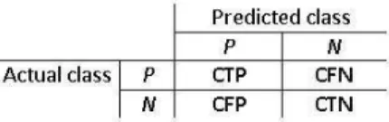
In this section, a new cost-sensitive self-training method CS-ST is presented. Here we focus on datasets with binary class. The main idea of CS-ST is to consider the expected cost when selecting and labeling the unlabeled instances so as to adapt the self-training algorithm to cost-sensitive learning problems. The degree of change of the average misclassification cost is used as a further selection criterion to decide whether to add the selected instances into the training data. To clearly illustrate the idea, a cost matrix for binary-class datasets is shown in Fig. 1. The class with lower misclassification cost is represented as positive (P ), and the class with higher misclassification cost as negative (N ). “CFP” is the cost of wrongly classifying a negative instance to be positive. “CFN” is the cost of misclassifying a positive instance to be negative. “CTP” and “CTN” are the costs of correctly classifying a positive instance and a negative instance,
respectively. Usually, CT P =CT N =0. We set CF N =1 and CF P > 1 because misclassifying a negative instance is associated with a larger cost. The average misclassification cost on a testing dataset with m instances can be formulated as: AC = Pmi=1C(predictedclassi, actualclassi)/m, where predictedclassi and
actualclassi are the predicted class label and the actual class label of the i-th
testing instance, respectively.
Fig. 1: Cost matrix for binary-class datasets
Input: labeled data L0 and unlabeled data U .
Output: a cost-sensitive classifier. 1. Set the iteration counter t to 0.
2. Build a Naive Bayes classifier C0 on the labeled data L0 only.
3. ComputeACft.
4. While the stopping criteria are not satisfied,
(a) Select m unlabeled instances from Ut that classifier Ct has the smallest
ex-pected cost.
(b) Assign each selected unlabeled instance an “optimum” label with the smallest the conditional risk computed by Equation 1.
(c) Form Lt+1as the union of Ltand the selected instances.
(d) Form Ut+1by deleting the selected instances from Ut.
(e) Build a Naive Bayes classifier Ct+1on Lt+1.
(f) ComputeACft+1.
(g) IfACft+1>ACft, Lt+1= Ltand Ct+1= Ct.
(h) Increase t by 1. 5. Return the final classifier.
Fig. 2: CS-ST Algorithm
The algorithm is given in Figure 2. Initially, a Naive Bayes classifier C0 is
learned from L0. In iteration t, Lt is updated and a new Naive Bayes classifier
Ctis built from Lt. The unlabeled instances are selected and labeled according
further decide whether to use the selected instances to expand the training data. Since the real labels of the unlabeled data are unknown to the algorithm, it is not feasible to compute the actual misclassification cost of the each classifier in each iteration. Therefore, we estimate the average misclassification cost of Cton
a small dataset with real labels (L0) in iteration t, denoted as gACt. gAC0 is the
average misclassification cost of C0 computed from L0. The stopping criterion
is that the maximum number of iterations is reached or there is no unlabeled instances left in U .
Compared to the standard self-training, the misclassification cost is consid-ered in three places:
– Selection (step 4(a)): after current classifier Ctproduces the prediction
prob-ability for each unlabeled instance, the conditional risk is computed using Equation 1. The m unlabeled instances with the smallest expected cost will be selected.
– Labeling (step 4(b)): for each of the m selected instance, assign it the “op-timum” class that has the smallest expected cost.
– Whether to accept the m instances to expand the labeled data in the next iteration (steps 4(e-f)): if gACt+1 > gACt, discard the m selected instances;
otherwise, use them in the next iteration.
3
Experiments and Results
In this section, CS-ST is compared with following approaches:
(1) SelfTrain it is the standard self-training method using Naive Bayes as the base classifier.
(2) SL it is a Naive Bayes classifier trained on the original labeled data only. For each method, after the classifier is built, testing instances are assigned labels according to the predicted probabilities of the classifier, and the average mis-classification cost is computed thereafter based on the number of misclassified instances and the corresponding costs.
3.1 Datasets
Two kinds of datasets are used to compare the performance of the methods. The first set is 13 datasets that appear in many papers about cost-sensitive learning [4] [15] [5] [14] [16]. They can be downloaded from UCI repository [1]. In our experiments, the datasets are pre-processed in Weka [18]. Missing values are replaced by the “ReplaceMissing” filter. Numeric values are discretized by the ten-bin discretization filter. The dataset “hypothyroid” is changed to a binary class dataset by selecting the two most frequent class values. The second set is three text datasets “oh0”, “oh5”, and “oh10” that are used in Qin [14].
To be consistent, the order of class values in some datasets are changed so that the majority (positive) class is the first class value while the minority
Table 1: Experimental Datasets
Dataset Size #Attr #Pos #Neg %Neg #Pos/#Neg breast-cancer 286 10 201 85 29.72% 2.4 breast-w 699 10 458 241 34.48% 1.9 bupa 345 7 200 145 42.03% 1.4 clean1 476 167 269 207 43.49% 1.3 credit-g 1000 21 700 300 30.00% 2.3 hypothyroid 3675 30 3481 194 5.28% 17.9 kr-vs-kp 3196 37 1669 1527 47.78% 1.1 pima-indians 768 9 500 268 34.90% 1.9 sick 3772 30 3541 231 6.12% 15.3 tic-tac-toe 958 10 626 332 34.66% 1.9 vote 435 17 267 168 38.62% 1.6 wdbc 569 31 357 212 37.26% 1.7 spambase 4601 58 2788 1813 39.40% 1.5 oh0 1003 3183 809 194 19.34% 4.2 oh5 918 3013 769 149 16.23% 5.2 oh10 1050 3239 885 165 15.71% 5.4
(negative) class is the second class value. The modified datasets include “tic-tac-toe”, “bupa”, “breast-cancer”, “breast-w”, and “vote”.
The details of the data sets are displayed in Table 1. “#Attr” is the number of attributes in each dataset. Columns “#Pos” and “#Neg” show the number of instances belong to positive class and negative class, respectively, in each dataset. Column “%Neg” depicts the percentage of negative instances in each dataset. And column “#Pos/#Neg” is the ratio of positive instances to negative instances in each dataset.
3.2 Experimental settings
On each dataset, ten runs of five-fold cross-validation are conducted and the average results are reported. The labeled percentage l% is set to be 1%. Hence, in each fold, 20% data is kept as the testing set, and the other 80% data is then randomly split into labeled data L0 (1% of the 80% data) and unlabeled data
U (99% of the 80% data). The class distribution in the labeled data is kept the same as that in the whole dataset.
We implemented CS-ST and self-training in Weka, and utilized the code for NaiveBayes and NaiveBayesMultinomial in Weka. For the 13 UCI datasets, NaiveBayes is used as the base classifier in all the methods. For the three text datasets, NaiveBayesMultinomial classifier is used as the base classifier because it is suitable for dealing with text datasets.
The cost of misclassifying a negative instance to be positive (CF P ) is set to 2, 5, and 10, respectively, in some cost-sensitive papers [4] [9] [16]. In our experiments, the same values are set to CF P to observe the performance of the three methods in different situations. The average misclassification cost is used as the performance measurement.
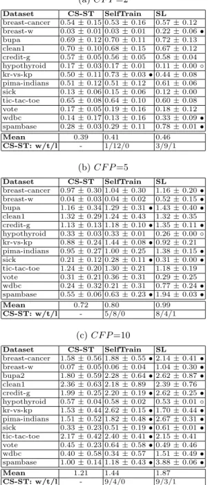
Table 2: Average results of the average misclassification cost on 13 UCI datasets (a) CF P =2 Dataset CS-ST SelfTrain SL breast-cancer 0.54 ± 0.15 0.53 ± 0.16 0.57 ± 0.12 breast-w 0.03 ± 0.01 0.03 ± 0.01 0.22 ± 0.06 • bupa 0.69 ± 0.12 0.70 ± 0.11 0.72 ± 0.13 clean1 0.70 ± 0.10 0.68 ± 0.15 0.67 ± 0.12 credit-g 0.57 ± 0.05 0.56 ± 0.05 0.58 ± 0.04 hypothyroid 0.17 ± 0.03 0.17 ± 0.01 0.11 ± 0.00 ◦ kr-vs-kp 0.50 ± 0.11 0.73 ± 0.03 • 0.44 ± 0.08 pima-indians 0.51 ± 0.12 0.51 ± 0.12 0.61 ± 0.06 sick 0.13 ± 0.06 0.15 ± 0.06 0.12 ± 0.00 tic-tac-toe 0.65 ± 0.08 0.64 ± 0.10 0.60 ± 0.08 vote 0.17 ± 0.05 0.19 ± 0.16 0.18 ± 0.12 wdbc 0.14 ± 0.17 0.13 ± 0.16 0.33 ± 0.09 • spambase 0.28 ± 0.03 0.29 ± 0.11 0.78 ± 0.01 • Mean 0.39 0.41 0.46 CS-ST: w/t/l - 1/12/0 3/9/1 (b) CF P =5 Dataset CS-ST SelfTrain SL breast-cancer 0.97 ± 0.30 1.04 ± 0.30 1.16 ± 0.20 • breast-w 0.04 ± 0.03 0.04 ± 0.02 0.52 ± 0.15 • bupa 1.16 ± 0.34 1.29 ± 0.31 • 1.43 ± 0.40 • clean1 1.32 ± 0.29 1.24 ± 0.43 1.32 ± 0.35 credit-g 1.13 ± 0.13 1.18 ± 0.10 • 1.35 ± 0.11 • hypothyroid 0.33 ± 0.03 0.33 ± 0.01 0.26 ± 0.00 ◦ kr-vs-kp 0.88 ± 0.24 1.44 ± 0.08 • 0.92 ± 0.21 pima-indians 0.95 ± 0.27 1.00 ± 0.25 1.38 ± 0.15 • sick 0.21 ± 0.12 0.28 ± 0.11 • 0.31 ± 0.00 • tic-tac-toe 1.24 ± 0.20 1.30 ± 0.21 1.18 ± 0.19 vote 0.31 ± 0.21 0.36 ± 0.31 0.29 ± 0.25 wdbc 0.24 ± 0.32 0.21 ± 0.31 0.77 ± 0.24 • spambase 0.55 ± 0.06 0.63 ± 0.23 • 1.94 ± 0.03 • Mean 0.72 0.80 0.99 CS-ST: w/t/l - 5/8/0 8/4/1 (c) CF P =10 Dataset CS-ST SelfTrain SL breast-cancer 1.58 ± 0.56 1.88 ± 0.55 • 2.14 ± 0.41 • breast-w 0.07 ± 0.05 0.06 ± 0.04 1.04 ± 0.30 • bupa2 1.80 ± 0.59 2.28 ± 0.64 • 2.62 ± 0.87 • clean1 2.36 ± 0.63 2.18 ± 0.89 2.39 ± 0.76 credit-g 1.99 ± 0.25 2.20 ± 0.19 • 2.62 ± 0.25 • hypothyroid 0.57 ± 0.04 0.58 ± 0.02 0.53 ± 0.01 ◦ kr-vs-kp 1.53 ± 0.44 2.62 ± 0.15 • 1.70 ± 0.44 • pima-indians 1.51 ± 0.52 1.82 ± 0.48 • 2.67 ± 0.31 • sick 0.33 ± 0.23 0.51 ± 0.19 • 0.61 ± 0.01 • tic-tac-toe 2.17 ± 0.42 2.40 ± 0.41 • 2.15 ± 0.41 vote 0.45 ± 0.23 0.64 ± 0.58 • 0.49 ± 0.46 wdbc 0.40 ± 0.58 0.34 ± 0.57 1.51 ± 0.49 • spambase 1.00 ± 0.14 1.18 ± 0.43 • 3.88 ± 0.06 • Mean 1.21 1.44 1.87 CS-ST: w/t/l - 9/4/0 9/3/1
3.3 Results on 13 UCI datasets
Comparison results of the methods when using different CF P values are shown in the sub-tables of Table 2. Each value in front of “±” is the average value of the average misclassification costs computed in the ten runs of five-fold cross-validation, followed by the corresponding standard deviation after “±”. Row “Mean” depicts the mean value of the average misclassification cost computed over all the datasets of the corresponding column. Row “CS-ST: w/t/l” repre-sents that CS-ST wins on w datasets (marked by •), ties on t datasets, and loses on l datasets (marked by ◦) against the corresponding method, under a two-tailed pair-wise t-test at 95% significance level. Please note that, lower average cost implies better performance.
It can be seen that, CS-ST always gets smaller average misclassification cost than SelfTrain when CF P changes from 2 to 10. It significantly outperforms self-train on nine datasets when CF P is 10. Moreover, CS-ST generally obtain much smaller average cost than SL except on the “hypothyroid” dataset. The advantage of CS-ST over SL is more obvious when CF P is 5 and 10.
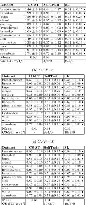
To compare the classifiers’s ability to identify negative instances, the com-parison results on True Negative Rate (TNR) are shown in Table 3. TNR is the ratio of the number of correctly classified negative instances over the total num-ber of negative instances. Higher TNR means that the classifier can identify more negative instances, which is beneficial to reduce the misclassifying cost. Because SelfTrain does not consider misclassification cost during classifier learning pro-cess, the classifier is the same when CF P changes and hence TNR values are not affected by using different CF P values. The situation is the same for SL.It can be observed from the table that, when CF P is small, CS-ST can win the other two methods on three or nine datasets while lose on two or one datasets. However, when CF P is 5 or 10, CS-ST significantly outperforms SelfTrain and SL on nine or ten datasets in terms of TNR.
To summarize the analysis, on the 13 UCI datasets, CS-ST generally has much better performance than SelfTrain and SL on most of the datasets con-cerning the average misclassification cost and the true negative rate, when CF P is 2, 5 or 10.
3.4 Results on three text datasets
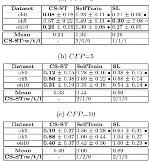
In [14], compared to a decision tree classifier built on the labeled data only and a direct-EM method, the presented method CS-EM shows better average misclassification cost only on “oh0 ” while obtaining similar results on ‘oh5 ” and “oh10 ”, when different CF P values are used. Here, we use the three text datasets to examine the performance of CS-ST. The comparison results on the average misclassification cost are shown in Table 4, when CF P is 2, 5, and 10, respectively.
It can be observed that, when CF P is 2, CS-ST significantly outperforms SelfTrain on all the three dataset. When CF P is larger, CS-ST significantly outperforms SelfTrain on one to two datasets, while having equal performance
Table 3: Average results of True Negative Rate on 13 UCI datasets (a) CF P =2 Dataset CS-ST SelfTrain SL breast-cancer 0.46 ± 0.18 0.44 ± 0.17 0.34 ± 0.15 • breast-w 0.99 ± 0.01 0.99 ± 0.01 0.70 ± 0.09 • bupa 0.56 ± 0.16 0.53 ± 0.16 0.43 ± 0.23 • clean1 0.51 ± 0.16 0.57 ± 0.22 ◦ 0.50 ± 0.19 credit-g 0.32 ± 0.08 0.32 ± 0.06 0.15 ± 0.09 • hypothyroid 0.06 ± 0.07 0.03 ± 0.03 • 0.00 ± 0.01 • kr-vs-kp 0.69 ± 0.09 0.51 ± 0.03 • 0.67 ± 0.10 pima-indians 0.55 ± 0.13 0.53 ± 0.13 0.26 ± 0.10 • sick 0.49 ± 0.34 0.25 ± 0.28 • 0.00 ± 0.01 • tic-tac-toe 0.38 ± 0.12 0.37 ± 0.12 0.44 ± 0.13 ◦ vote 0.89 ± 0.07 0.86 ± 0.14 0.90 ± 0.11 wdbc 0.91 ± 0.14 0.93 ± 0.14 ◦ 0.60 ± 0.14 • spambase 0.74 ± 0.04 0.72 ± 0.10 0.02 ± 0.01 • Mean 0.58 0.54 0.39 CS-ST: w/t/l - 3/8/2 9/3/1 (b) CF P =5 Dataset CS-ST SelfTrain SL breast-cancer 0.50 ±0.17 0.44 ±0.17 • 0.34 ±0.15 • breast-w 0.99 ±0.01 0.99 ±0.01 0.70 ±0.09 • bupa 0.62 ±0.18 0.53 ±0.16 • 0.43 ±0.23 • clean1 0.52 ±0.15 0.57 ±0.22 0.50 ±0.19 credit-g 0.38 ±0.09 0.32 ±0.06 • 0.15 ±0.09 • hypothyroid 0.06 ±0.08 0.03 ±0.03 • 0.00 ±0.01 • kr-vs-kp 0.73 ±0.10 0.51 ±0.03 • 0.67 ±0.10 • pima-indians 0.58 ±0.14 0.53 ±0.13 • 0.26 ±0.10 • sick 0.55 ±0.35 0.25 ±0.28 • 0.00 ±0.01 • tic-tac-toe 0.42 ±0.12 0.37 ±0.12 • 0.44 ±0.13 vote 0.88 ±0.11 0.86 ±0.14 0.90 ±0.11 wdbc 0.91 ±0.14 0.93 ±0.14 0.60 ±0.14 • spambase 0.77 ±0.04 0.72 ±0.10 • 0.02 ±0.01 • Mean 0.61 0.54 0.39 CS-ST: w/t/l - 9/4/0 10/3/0 (c) CF P =10 Dataset CS-ST SelfTrain SL breast-cancer 0.56 ±0.18 0.44 ±0.17 • 0.34 ±0.15 • breast-w 0.99 ±0.01 0.99 ±0.01 0.70 ±0.09 • bupa 0.66 ±0.15 0.53 ±0.16 • 0.43 ±0.23 • clean1 0.52 ±0.15 0.57 ±0.22 0.50 ±0.19 credit-g 0.41 ±0.09 0.32 ±0.06 • 0.15 ±0.09 • hypothyroid 0.07 ±0.09 0.03 ±0.03 • 0.00 ±0.01 • kr-vs-kp 0.73 ±0.09 0.51 ±0.03 • 0.67 ±0.10 • pima-indians 0.64 ±0.14 0.53 ±0.13 • 0.26 ±0.10 • sick 0.60 ±0.35 0.25 ±0.28 • 0.00 ±0.01 • tic-tac-toe 0.45 ±0.13 0.37 ±0.12 • 0.44 ±0.13 vote 0.91 ±0.06 0.86 ±0.14 • 0.90 ±0.11 wdbc 0.91 ±0.14 0.93 ±0.14 0.60 ±0.14 • spambase 0.77 ±0.04 0.72 ±0.10 • 0.02 ±0.01 • Mean 0.63 0.54 0.39 CS-ST: w/t/l - 10/3/0 10/3/0
Table 4: Average results of the average misclassification cost on three text datasets (a) CF P =2 Dataset CS-ST SelfTrain SL oh0 0.08 ± 0.08 0.23 ± 0.11 • 0.21 ± 0.06 • oh5 0.37 ± 0.22 0.49 ± 0.11 • 0.30 ± 0.08 ◦ oh10 0.26 ± 0.09 0.30 ± 0.08 • 0.27 ± 0.05 Mean 0.24 0.34 0.26 CS-ST:w/t/l - 3/0/0 1/1/1 (b) CF P =5 Dataset CS-ST SelfTrain SL oh0 0.12 ± 0.15 0.28 ± 0.16 • 0.38 ± 0.15 • oh5 0.56 ± 0.38 0.69 ± 0.22 • 0.58 ± 0.14 oh10 0.31 ± 0.19 0.35 ± 0.18 0.54 ± 0.14 • Mean 0.33 0.44 0.50 CS-ST:w/t/l - 2/1/0 2/1/0 (c) CF P =10 Dataset CS-ST SelfTrain SL oh0 0.19 ± 0.27 0.36 ± 0.28 • 0.64 ± 0.31 • oh5 0.88 ± 0.67 1.00 ± 0.44 1.04 ± 0.27 oh10 0.40 ± 0.37 0.42 ± 0.36 1.00 ± 0.29 • Mean 0.49 0.60 0.89 CS-ST:w/t/l - 1/2/0 2/1/0
on the other datasets. While CS-ST wins on one dataset and loses on one dataset over SL when CF P is 2, the former significantly outperforms the latter on two datasets and ties on one dataset when CF P is 5 and 10. In other words, when CF P is larger, CS-ST can have more effect to reduce the misclassification cost than the other two methods.
In each row, the lowest average misclassification cost obtained on the dataset is shown in bold font. It is observed that, CS-ST generally obtains the lowest average misclassification cost among the four methods except on “oh5” when CF P is 2. Moreover, CS-ST has much lower mean values on the three datasets than the other two methods. The difference is more obvious when CF P is 10.
Therefore, on the three text datasets, CS-ST also generally outperforms Self-Train and SL on the average misclassification cost when CF P is 2, 5 or 10. The superior performance is obviously observed when CF P is larger.
4
Conclusions and Future Work
In this paper, we present a cost-sensitive self-training method CS-ST to deal with the situation that the number of labeled data is small and different mis-classification errors incur different costs. Naive Bayes is used as the underlying classifier. The expected cost is considered when selecting and labeling unlabeled
instances in each iteration of self-training. In order to prevent possible perfor-mance degradation, the change of perforperfor-mance on average misclassification cost on the original labeled data is applied to decide whether to add the selected in-stances to expand the training data. Our experimental results on 13 UCI datasets and three text datasets show that, with different misclassification costs, CS-ST generally outperforms two base methods in terms of the average misclassification cost and the true negative rate. The advantage of CS-ST is more obvious when the misclassification cost increases.
In the future, we will try ensemble learning, sampling, or threshold strategies in semi-supervised learning to further improve the performance on average cost on the UCI datasets. The method may also be extended to apply on multi-class datasets.
References
1. UCI Machine Learning Repository, http://archive.ics.uci.edu/ml/datasets. html
2. Abe, N., Zadrozny, B., Langford, J.: An iterative method for multi-class cost-sensitive learning. In: Proc. 10th ACM SIGKDD International Conference on Knowledge Discovery and Data Mining. pp. 3–11 (2004)
3. Chapelle, O., Sch¨olkopf, B., Zien, A. (eds.): Semi-supervised learning. MIT Press, Cambridge, MA (2006)
4. Domingos, P.: MetaCost: A general method for making classifiers cost-sensitive. In: Proc. 5th ACM SIGKDD International Conference on Knowledge Discovery and Data Mining. pp. 155–164 (1999)
5. Donmez, P., Carbonell, J.G.: Proactive learning: Cost-sensitive active learning with multiple imperfect oracles. In: Proc. 17th ACM Conference on Information and Knowledge Management (2008)
6. Elkan, C.: The foundations of cost-sensitive learning. In: Proc. 17th International Joint Conference on Artificial Intelligence. pp. 973–978 (2001)
7. Guo, Y., Zhang, H., Liu, X.: Instance selection in semi-supervised learning. In: Proc. 24th Canadian Conference on Artificial Intelligence. pp. 158–169 (2011) 8. Li, M., Zhou, Z.H.: SETRED: self-training with editing. In: Proc. Advances in
Knowledge Discovery and Data Mining. pp. 611–621 (2005)
9. Li, Y.F., Kwok, J.T., Zhou, Z.H.: Cost-sensitive semi-supervised support vector machine. In: Proc. 24th AAAI Conference on Artificial Intelligence. pp. 500–505 (2010)
10. Liu, A., Jun, G., Ghosh, J.: A self-training approach to cost sensitive uncertainty sampling. Machine Learning 76, 257–270 (2009)
11. Liu, X.Y., Zhou, Z.H.: The influence of class imbalance on cost-sensitive learning: An empirical study. In: Proc. 6th IEEE International Conference on Data Mining. pp. 970–974 (2006)
12. Margineantu, D.D.: Active cost-sensitive learning. In: Proc. 19th International Joint Conference on Artificial Intelligence (2005)
13. Muslea, I., Minton, S., Knoblock, C.A.: Active + semi-supervised learning = robust multi-view learning. In: Proc. 19th International Conference on Machine Learning (2002)
14. Qin, Z., Zhang, S., Liu, L., Wang, T.: Cost-sensitive semi-supervised classifica-tion using CS-EM. In: Proc. 8th IEEE Internaclassifica-tional Conference on Computer and Information Technology. pp. 131–136 (2008)
15. Sheng, V.S., Ling, C.X.: Thresholding for making classifiers cost-sensitive. In: Proc. 21st National Conference on Artificial Intelligence (AAAI-06) (2006)
16. Ting, K.M.: A comparative study of cost-sensitive boosting algorithms. In: Proc. 17th International Conference on Machine Learning. pp. 983–990 (2000)
17. Wang, B., Spencer, B., Ling, C.X., Zhang, H.: Semi-supervised self-training for sentence subjectivity classification. In: 21st Canadian Conference on Artificial In-telligence. pp. 344–355 (2008)
18. Witten, I.H., Frank, E. (eds.): Data mining: Practical machine learning tools and techniques. Morgan Kaufmann, 2nd edn. (2005)
19. Yarowsky, D.: Unsupervised word sense disambiguation rivaling supervised meth-ods. In: Proc. 33rd Annual Meeting of the Association for Computational Linguis-tics. pp. 189–196 (1995)