Big data fusion to estimate driving adoption behavior and urban fuel consumption

Big Data Fusion to Estimate Driving Adoption Behavior

and Urban Fuel Consumption

by

Adham Kalila

B.Eng, McGill University (c012)

Submitted to the Department of Civil and Environmental Engineering

in partial fulfillment of the requirements for the degree of

Master of Science in Transportation

at the

MASSACHUSETTS INSTITUTE OF TECHNOLOGY

June 2018

@ Massachusetts Institute of Technology 2018. All rights reserved.

Signature redacted

A u th o r ...

...

Department of Civil and Environmental Engineering

May 18, 2018

C ertified by ...

Signature redacted

Marta C. Gonzalez

Associate Professor of Civil and Environmental Engineering

Thesis Supervisor

A

A ccepted by ...

IMASSACHUSEIS

~TUT

I

OFrTECHNOfsGYs_{MAS AC USI- SINSIT TE}

P rofessor of(

C

Signature redacted

/

Jesse Kroll

Civil and Environmental Engineering hair, Graduate Program Committee

JUL 26 2018

LIBRARIES

Big Data Fusion to Estimate Driving Adoption Behavior and

Urban Fuel Consumption

by

Adham Kalila

Submitted to the Department of Civil and Environmental Engineering on May 18, 2018, in partial fulfillment of the

requirements for the degree of Master of Science in Transportation

Abstract

Data from mobile phones is constantly increasing in accuracy, quantity, and ubiquity. Meth-ods that utilize such data in the field of transportation demand forecasting have been pro-posed and represent a welcome addition. We propose a framework that uses the resulting travel demand and computes fuel consumption. The model is calibrated for application on any range of car fuel efficiency and combined with other sources of data to produce urban fuel consumption estimates for the city of Riyadh as an application. Targeted traffic conges-tion reducconges-tion strategies are compared to random traffic reducconges-tion and the results indicate a factor of 2 improvement on fuel savings. Moreover, an agent-based innovation adoption model is used with a network of women from Call Detail Records to simulate the time at which women may adopt driving after the ban on females driving is lifted in Saudi Arabia. The resulting adoption rates are combined with fuel costs from simulating empty driver trips to forecast the fuel savings potential of such a historic policy change.

Thesis Supervisor: Marta C. Gonzilez

Acknowledgments

I could not have completed this masters without the love, encouragement, and support of

my family, friends, and advisors.

To my thesis advisor and mentor, Marta C. Gonzdlez, who took a chance on me and patiently taught me the ins and outs of not just research but MIT and the academic world

in general, thank you.

To my unofficial advisor, Sarah Williams, who continues to inspire in me a love of public transportation and mapping, thank you.

To my friends, my Cantabrigian family, your support through the ups and downs of such a unparalleled place as MIT was not only wonderful but essential.

To my friends from Cairo, my shella sha2eya, your faith in my abilities kept me going even when I had lost faith in myself.

To my family, especially my mother Mona, your life inspires me to achieve more and more. To my brother Amir, I will always be grateful for the ways you have enabled me to be here.

To the Massachusetts Institute of Technology, I am forever grateful for your lasting effect on my professional, personal, and academic life.

Contents

1 Introduction

1.1 Overview and Motivation . . . . 1.2 Literature Review . . . . 1.2.1 Travel Demand and Call Detail Records . . . .

1.2.2 Fuel Consumption Estimation Models . . . .

1.2.3 Social Diffusion Adoption Models . . . .

1.3 Thesis O utline . . . .

2 Calibrating the Fuel Consumption Model

2.1 Introduction . . . .

2.2 StreetSmart Model Sensitivity Analysis . . . .

2.3 Results and Energy Indices . . . .

3 Fuel Consumption Application for Traffic Congestion 3.1 M ethodology . . . . 3.1.1 Froni GPS Data to Speed Profiles . . . . 3.1.2 Fuel Consumption Results . . . ... . . . .

3.2 Discussion and Conclusion . . . .

4 Fuel Effects of Women Adopting Driving in Riyadh 4.1 Introduction . . . .

4.2 Data Description: CDR and Gender labeled Users . . . 4.2.1 Data description . . . . Policies 15 15 17 17 18 19 21 23 23 24 25 31 32 32 35 40 43 43 44 44 . . . . . . . . . . . .

4.2.2 Gender Labeling . . . .

4.2.3 Expansion Factors . . . .

4.3 Trip Generation and Fuel Consumption Methods 4.3.1 Trip Generation and flows . . . . 4.3.2 Driver Trip Simulation . . . . 4.4 Calculating Fuel Consumption . . . . 4.4.1 Fuel Consumption Model . . . . 4.4.2 Verification of Aggregate Fuel Results . . .

4.4.3 Model of Adoption of Driving by Women . 4.5 Discussion and Conclusion . . . . 4.5.1 Limitations and Assumptions . . . . 4.5.2 Policy Recomendations . . . .

5 Conclusion

5.1 Summary . . . .

5.2 Limitations of the Framework . . . .

5.3 FutureWork. . . . . . . . . 45 . . . . 45 . . . . 46 . . . . 46 . . . . 50 . . . . 51 . . . . 51 . . . . 52 . . . . 54 . . . . 56 . . . . 56 . . . . 58 59 59 60 61

List of Figures

1-1 Stay and pass-by identification from filtered points showing home and work location examples. Source: (1) . . . . 18

1-2 Everett Rogers' innovation adoption curve showing the difference between early, middle, and late adopters. Source: (40) . . . . 20 2-1 Values of Energy Indices k resulting from the regression of fuel consumption

and speed profiles in the Illinois experiment . . . . 25

2-2 Sensitivity Analysis of k parameters. Values of k are varied individually while

the other indices are set such that fuel efficiency is at 20.5 mpg and the result on fuel efficiency is graphed . . . . 26 2-3 Speed profiles showing idle and moving times. Source: StreetSmart

experi-m ent (50) . . . . 27

2-4 Department of Energy Fuel Efficiency vs Average Speed Curve (52) . . . . . 28 2-5 (a) FTP-75 EPA's standard speed profile used for calculating the reported

inner-city fuel economies of cars. (b) The distribution of fuel economies recre-ated by the StreetSmart model shows the same distribution as that of the reported fuel economies. (c) The distribution of fuel economies based on Rivadhi's fleet of cars compared to those of Poland and the UK shows that the distributions are similar but shifted from one another. The car fleet of Riyadh is less fuel efficient than that of Poland which is less than that of the

U K . . . . 2 8

3-1 Average hourly taxi trip production rates in Riyadh in Ramadan., non-Ramadan, and com bined. . . . . 33

3-2 Data Verification figures using trips in the morning peak time period of

week-days from 8 -9 AM. (a) Histogram of Reported and calculated Trip Distances. (b) Histogram of free flow travel time and Observed travel time in matched

trips. (c) _{Histogram of Fuel economies using constant speed, speed profiles,}

and 1 bin and all bins. . . . . 35

3-3 Choropleth Maps of fuel consumption rates

[Liter/meter.hour]

by the StreetS-mart model on streets matched with GPS data for typical time periods

morn-ing peak (8 - 9 AM) weekdays, midday off-peak (12 - 13 PM) weekdays,

evening peak (17 - 18 PM) weekdays. . . . . 37

3-4 Fuel consumption estimates at urban scale. (a) Comparison of the travel time of the routes in the constant speed model via travel demand vs. the input used in our method using GPS data (b) Sample speed profiles in two routes used to estimate fuel consumption overlaid with the constant speed used for comparison (c) Estimates of fuel consumption and fuel economy in the morning peak via our method (speed profiles) and the base line method (constant speed) (d) Random and targeted fuel savings vs. number of reduced trip s. . . . . 3 9

4-1 Expansion Factors of CDR users, (a) Choropleth map of expansion factors for all CDR users, (b) Choropleth map of expansion factors for gender-labeled

CDR, users, (c) distribution of expansion factorsfor all CDR, users., (d) scatter

of CDR population vs census population for every TAZ in blue and after

expansion in red, (e) ditribution of expansion factors for gender-labeled CDR users, (f) scatter of CDR population vs census population for every TAZ by gender ... ... 47

4-2 Features of Mobility by Gender, (a) a Joyplot showing the trip departure time distribution for male and female users by trip purpose HBW,HBO,an NHB compared to the distribution from the NHTS, (b) A map of the home and

work locations of users colored by gender, (c) outer: Average locations visited

per day by gender, inner: Lth most visited locations by gender, (d) Radius of Gyration and Average Stay Duration distributions by gender, (e) Mobility Diversity distribution by gender . . . 48 4-3 Driver Trip Simulation, (a) Departure time distribution of empty driver and

essential female trips, (b) diagram of the relation between empty driver and essential fem ale trips . . . . 51

4-4 Morining Trip Simulation Verification Diagrams, (a) Boxplots of trip simu-lation times [mini], distances [ki], and fuel consumption [liter] with median shown, (b) distribution of fuel efficiency of each trip, (c) scatter of GPS-recorded total trip time vs ITA congested trip times . . . . 53

4-5 Network and Adoption Scenario Results, (a) degree distribution of the female gender-labeled CDR users network of communications and the largest coin-ponent in the network visualized, (b) Adoption Scenarios and their associated

List of Tables

2.1 A Comparison of Fuel Consumption Estimates from the StreetSmart Model

and the DOE Fuel Economy Fit on Data From the Experiment Conducted by (5 1 )) . . . . 2 7

2.2 Results of the Calibration of the StreetSmart Model. Ranges of ki Parameters for Each Bin of Fuel Economy . . . . 29

4.1 Percent of Trips by Purpose and Time of Day Compared to NHTS and MHTS 49 4.2 Fuel Consumption Estimation Totals for Male and Female and Empty Driver

Chapter 1

Introduction

1.1

Overview and Motivation

This thesis is the product of several motivations on my part and on the part of my advisor, Prof. Marta Gonzalez. First, it is an attempt to build upon the travel demand computed from Call Detail Records (CDRs) to estimate fuel consumption and show that the ubiquity of data being produced today has uses far beyond its original intention. Second, it is a scientific exercise in modeling the effects of the liberalization of restrictions on women driving in Saudi Arabia. The results show how we can start from several disparate data sources, combine them with a framework and human simulation model to produce tangible results that are then verified against state of the art techniques and ground truths.

The reason the methods outlined below are pertinent and realistic is thanks to the wealth of data being collected from mobile phones today. With penetration rates of over

85% in developing countries and up to 100% in some developed countries, mobile phones

are constantly and precisely recording our movement and our lives. This is a far cry from the level of data that is used in a household travel survey which depicts a typical day and cannot robustly consider the effects of weather, holidays, and other day-today factors on travel demand. In order to harness useful insights from such new data, we must develop techniques that utilize its potential. Apart from straight forward origin-destination (OD) travel demand which is used in infrastructure decisions, environmental studies, etc. such data can also be used to answer specific policy questions through simulation and modeling

human behavior.

The motivation to compute travel demand from Big Data sources such as mobile phone traces or CDRs comes as a response to the difficult alternative of building discrete choice models and conducting expensive and time-consuming stated preference surveys. Pre-vious work has shown that these new techniques, such as TimeGeo (1), are faithful to the state of the art methods and verified against real surveys and accepted truths. We extend the current framework which identifies stays, generates trips, and estimates travel demand, to add the ability to estimate fuel consumption. This energy consideration comes at a time when oil-producing countries are suffering from the low prices of oil since 2016. Saudi Arabia's economy is undergoing immense changes to diversify its economy and decrease its reliance upon the price of one commodity. For this reason, we have developed a framework to accurately estimate urban fuel consumption.

The methods are also applied to simulate the possible fuel savings potential of women starting to drive in Saudi Arabia. Since the 1970s, women have been banned from driving for cultural and supposedly religious reasons. There were some protests by activist women in the 1990s but they were immediately put down. With the recent increase in young Saudis returning after studying abroad, the ruling family, especially the young crown prince Mohamed Bin Salman, is looking to appease the new generation and improve Saudi Arabia's international reputation. One of the new changes is the promise that the ban on women driving will be lifted in June 2018. We take advantage of the fuel consumption framework we developed as well as gender-identified subset of users to simulate the empty driver trips generated around women's mobility needs. With these we apply a diffusion model similar to the spread of disease or the adoption of a new technology in the market to relate the fuel savings with time under several scenarios.

The methods used utilize and contribute to the current knowledge in three distinct areas: Energy consumption with GPS, travel demand from CDR, and adoption modeling for women driving for the first time. The contributions of this thesis are summed up as follows: First, we calibrated a previously developed fuel consumption model (StreetSmart) and applied it to varying fuel efficiencies in car fleets; Second, the model was used along with travel demand estimated by CDR-based traffic assignment to approximate fuel consumption

rates in Riyadh, Saudi Arabia; Third, we examined the effects of the proposed method by comparing the effects on fuel consumption of different traffic relief policies; Fourth, we model the associated empty driver trips made to accommodate the ban on women driving in Saudi Arabia and model the fuel savings potential of the adoption of driving after the ban is lifted. The following section outlines the previous knowledge and where the current thesis fits into it.

1.2

Literature Review

1.2.1

Travel Demand and Call Detail Records

The traditional engineering method of estimating travel demand used travel diaries and sur-veys and followed a four-step model. Trip generation, trip distribution, mode choice, and trip assignment produced an origin-destination flow matrix aggregated by Traffic Analysis Zone (TAZ). Since then, improved computing has enabled trip-based modeling to capture more idiosyncrasies and individual-level variations in the data. Ever increasing storage capacity and faster processing, both local on hand-held devices as well as cloud-based, has resulted in incredibly massive amounts of data such as location, elevation, purchases, tweets, check-ins, and even heart-rate to be stored and logged for billions of people around the planet.

Data collected by telecommunications providers for billing purposes has been used to shed light on human urban mobility since it was found that humans have very predictable routines and are slow to discover new places (2). For the purposes of transportation, algo-rithms and methods for stay extraction (3), OD extraction and validation (4-7), travel speed estimation (8, 9) and activity modeling (10, 11) have been developed to benefit from CDR data. An example of home and work identification from stay and pass-by locations is shown in Figure 1-1.

CDR typically contains a timestamp, location coordinates, duration of the call or text, and a unique identifier for the user. The coordinates in the CDR records obtained from the city of Riyadh, Saudi Arabia for this project were of the cell towers used by the phone and not of the phones themselves. This resulted in an OD model aggregated at the TAZ

0 3.5 7 KM 0 3.5 7 KM 0 3.5 7 KM

G" + I i H&1 rA oes Im"k a

G

H*I

Q*

mass assu anna ny (omm)

2.2% 12%

Slay (ork)

SStay (Other 2) -0D link

Fiur 11 * A%.pAi 250 Previous Stays

Revious 00 ENrs

Figure 1-1: Stay and pass-by identification from filtered points showing home and work location examples. Source: (1)

level and greatly simplified the analysis. The TimeGeo framework (1), which in turn was built on previous work on CDR (12, 13), is the basis from which the OD flows used in this project are derived. A summary of how trip generation is derived from the CDR records is as follows. First, stays are identified apart from pass-by points as locations where the user spent a significant time within a threshold radius. Based on the time and frequency of the stay locations, they are labeled as one of home, work, or other. This label feeds into a heuristic that informs the trip generation. For example, users start and end each day at their home location and they commute to work with a departure time drawn from local and national household travel surveys. Once all trips have been generated the flows that they represent,

based on how often a user is observed in the dataset, are then iteratively assigned to roads and the resulting traffic flows are calculated. This work describes using the resulting flows in conjunction with speed profiles observed from a high frequency GPS dataset to estimate fuel consumption on roads.

1.2.2

Fuel Consumption Estimation Models

The estimation of energy consumption from location data is prevalent in the literature with several models that utilize different factors. Since smartphone market penetration is almost complete in the Transportation Networking Companies (TNCs) industry (14), GPS tracking

has been successfully used to estimate air pollution (15), instantaneous fuel consumption

(16-20), and traffic conditions (21-25). Most studies that use GPS data to estimate fuel

Fuel consumption and emissions models have been extensively developed in the liter-ature (26-33). They are generally split between models that estimate the fuel consumption

by balancing the engine's carbon intake and combustion and those that attempt to use

mode-specific variables, such as speed and acceleration, to fit a model that estimates fuel consumption (32). Of those models that use instantaneous mode-specific variables, some estimate air pollution and emissions(15, 27, 28, 30), fuel consumption (18-20, 31) or both

(16, 17, 29). Most previous attempts at estimating instantaneous fuel consumption and

emissions do not incorporate GPS data but rely instead on On-Board Diagnostics devices (OBD-II) that measure fuel consumption and emissions (16-18, 29). The models that have attempted to use GPS data to estimate fuel consumption do so without consideration to the different fuel economies found in today's cars (19, 20, 31) and do not account for the total demand.

Our foray into fuel consumption aims to contribute to this evident lack in the frame-work. GPS data is used to compute fuel consumption rates per street for a variety of car fuel economies. This is then combined with traffic flows from an optimization algorithm to give a comprehensive picture of urban fuel consumption for an entire city, by time of day. This framework is then applied to Riyadh for verification and analysis.

1.2.3

Social Diffusion Adoption Models

The study of diffusion stems from rural sociology in the early 20th century and was solidified

by a study on the spread of hybrid seed corn in rural Iowa (34). In 1969, Bass published a

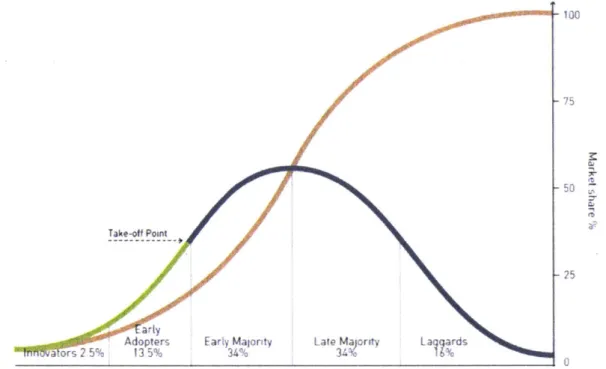
paper outlining the detail of what will become the most popular diffusion model. It assumes that potential adopters are influenced into adopting by innovation and imitation. Innovation can be the result of a media campaign whereas imitation comes from the interaction with other people. The resulting S-curve shows a distinction between the adoption of the phe-nomenon by early adopters, early and late majority adopters, and finally laggards. The Bass diffusion model takes as input aggregate numbers and its results are also aggregated and thus do not take into account the individual interactions between people or nodes. To make use of the social networks that are represented in telecommunication records (phone, text, email or social media), several studies have been conducted to simulate diffusion on an agent

based level (35-39). This new framework has been proposed in the literature which leverages network information for the imitation parameter, the threshold of probability above which a node decides to adopt. These have been more successful than the differential equation framework at describing diffusion with the Bass diffusion model.

-100 75 4 50 Takeoft Point 25 arty

Adopters Early majry Late Ma ority La ards

a ors 2.5% %4%3%

Figure 1-2: Everett Rogers' innovation adoption curve showing the difference between early, middle, and late adopters. Source: (40)

The parameters used for the Bass diffusion curve are the main area of debate when using the model for a particular product or phenomenon. Since the adoption of driving for the first time has never been recorded, electric car sales offer a reasonable proxy for its parameters. A summary of the sources of parameter values was compiled by Massiani and Gohs (41). They have found that a considerable number of papers and studies use previous parameters than are based on little more than conjecture by an expert (42-45). Other sources of parameter values can be non-peer reviewed such as Masters theses or reports from the private sector (46). Finally, when observable data is unavailable for a certain product in a specific market, similar markets or products are used as a proxy and parameters are fitted to observed sales data (47-49). Based on the results of the study by Massiani and Gohs, several scenarios of parameters were chosen to represent the adoption of Saudi women. A couple

of scenarios were added to mathematically model the results of surveys where women were asked about when they intended to drive, if at all, once the ban is lifted. This is presented in Chapter 4.4.

1.3

Thesis Outline

The remainder of this thesis presents a framework to utilize GPS and CDR to compute fuel calculation and test several policy application in Riyadh, Saudi Arabia.

Chapter 2 describes the method used to calibrate a model which uses speed profile (or driving schedules) to estimate fuel consumption given certain parameters. The process uses the results of an experiment where several cars outfitted with On Board Diagnostic Devices were driven around a track and their fuel consumption as well as their speed profiles were recorded. The model was calibrated for every type of fuel efficiency by categorizing vehicles, including motorcycles, buses and trucks, into 14 fuel efficiency ranges or bins. Parameter values for each bin were derived and later used on a real world application in Riyadh.

Chapter 3 presents the framework developed for fuel estimation from the model and applied to several traffic reduction policy scenarios. It was published as a paper in the Transportation Research Record in 2018.

Chapter 4 applies the fuel consumption framework on a subset of women and the empty driver trips that they incur. The travel demand of the city of Riyadh is used to compute the total urban fuel consumption which is verified against official reports and com-parable cities. Moreover, driver trips were simulated and their fuel consumption calculated. The Adoption of driving by women is modeled in 4 different scenarios and the associated fuel savings from avoided empty driver trips are computed.

Chapter 5 presents the conclusion and summary of findings as well as areas of potential future work.

Chapter 2

Calibrating the Fuel Consumption Model

2.1

Introduction

Fuel consumption is the result of the function of the power needed by the vehicle to overcome resistance integrated over time. This relationship between fuel and the variables that describe the vehicle and its movement is fit into a simple yet comprehensive model. The StreetSmart model was developed in 2011 at MIT to utilize accurate mobile phone sensor data to predict fuel consumption. It is part of a growing body of work that leverages GPS and Wi-Fi sensors on mobile phones to measure traffic. It goes beyond other efforts by using speed profiles with acceleration information over just average speed along a trip. The model fits data on the speed profiles to approximate four energy indices that capture different aspects of fuel consumption in a vehicle trip. The variables in the power function that are dependent on a vehicle's characteristics such as area, mass, accessories, etc. are replaced by these energy indices which are estimated by regression. For this project, we used the measured fuel consumption and speed profiles reported by an experiment conducted at the University of Illinois to get initial values for these energy indices.

The Illinois experiment analyzed and smoothed the speed profile data of four cars driven around a track with stop-and-go movements. The dataset contained raw video data as well as files with measured performance properties such as speed, acceleration, fuel effi-ciency, air mass flow rate etc. For our purposes, the data used were speed, time, and fuel consumption. The experiment consisted of 9, and sometimes 10, different cars driven around

a 30 meter diameter track. The next section will provide details on how we used the raw data to estimate energy indices of the StreetSmart model for 14 ranges or bins of fuel efficiency in cars.

2.2

StreetSmart Model Sensitivity Analysis

The StreetSmart model was developed by measuring the energy required by vehicles for vari-ous movement conditions. It estimates the fuel consumption with data from GPS coordinates from smartphones and ground truth fuel consumption data from On Board Diagnostics II (OBD-II) devices. Using the details of a trip's speed profile, the model successfully predicts fuel consumption with over 96% accuracy

[261,

a substantial improvement over models that only consider constant average speeds. Average speed estimations do not account for the stop and go effect of traffic, which is a significant factor leading to an increase in fuel con-sumption. In other words, average speed simplification results in lower, or more optimistic, fuel consumption estimates since drag is lower at low speeds.

After testing different variables for their use in predicting fuel consumption, the model employs a combination of four variables to predict fuel consumption as shown in 2.1. The first term accounts for energy wasted while the car is idling with the engine turned on; the second accounts for energy used with time spent moving; The third accounts for energy used due to acceleration and deceleration over a distance; the fourth accounts for energy used with distance traveled. Each term is multiplied by a specific energy index, ki, which depends on the vehicle efficiency, such that:

FC = k1Tidle + k2Tmove + k3 J |adx + k4L; (2.1)

where FC is fuel consumption in US gallons and ki,k2,k3, and k4 are the energy indices

calibrated with data separately for each bin of vehicle efficiency. Tidle and T,,v, are time

spent idling and moving respectively in seconds, a is acceleration in m/s2, and L is the distance driven in km.

The energy indices varied between the different models of cars. A chart of their difference is shown in Figure 2.1. To understand the effect on fuel consumption of each

Mff *asad ; "T TOOMCM-W Wffvd a : MTRWOX6 0 7 Cftraw OMNaFmd = 09mumm _{1 4} 045 4-1

Figure 2-1: Values of Energy Indices k resulting from the regression profiles in the Illinois experiment

of fuel consumption and speed

energy index alone, a sensitivity analysis was conducted where each index was varied between its observed minimum and maximum while keeping the other 3 such that fuel efficiency is at the average of 20.5 miles per gallon (mpg). The results on the fuel efficiency are shown in Figure 2.2. It was found that the change in fuel efficiency for each index was 3.5, 15.1, and 26 mpg respectively. Evidently, fuel efficiency is less sensitive to k, and k3 and more

sensitive k2 and k4.

2.3

Results and Energy Indices

Following (50), we further tested the StreetSmart model's indices by regression of the idle fuel consumption and moving fuel consumption separately using data from an experiment conducted at the University of Illinois by [27]. A graph of speed profiles showing idle and moving times is showin in Figure 2-3. To verify the benefit of using the model, its results were compared to a baseline estimation using average speed and the United States' Depart-ment of Energy's (DOE) graph of fuel economy variations by speed as shown in Figure 2-4. The StreetSmart model achieved inaccuracies of about 4% while the baseline method had inaccuracies of up to 29%. The details of the comparison are summarized in Table 2.1.

'''F

I

.. 11M 0.03 0-M MW0 -MU]1 -.00 0 amijoir-1 I

25 21.5-21 20.5 CL 20 w 19.5 LL 19- 18.5-18 17.50 _{3 3.5 4} x10-4 N-1 1.5 2 2-5 3 3.5 4 4.5 5 k3 x10" 5 247 22-20 10a216

-L

1412 10 -08 40 30 a 25, uJ U- 20i-0 0005 0.01 0.015 0.02 k4 4 5 6 x10-4 0.025 0.03 0.035

Figure 2-2: Sensitivity Analysis of k parameters. Values of k are varied individually while the other indices are set such that fuel efficiency is at 20.5 mpg and the result on fuel efficiency is graphed

To apply the StreetSmart model on a known distribution of car fuel economies, the first step is to relate the energy indices specific to each car fuel efficiency or economy. The variables with the highest influence over fuel consumption were the second and fourth indices representing time moving and the distance traveled respectively. This suggests that the first and third terms, representing the influence of speed profiles, have a lower impact on the overall estimate of fuel consumption. However, results shown in section 3.3 show that all

terms are useful since speed profiles improve the accuracy of estimation.

To calibrate the model and get energy index values for use on the scale of a city, we used the fuel economies reported by the Environmental Protection Agency's (EPA) 2016

0.5 1 1.5 2 25 k, 21.2 - 21- 20.8-2 20.6S20.4 - 20.2-20 19.805 1 2 3 k2

Oulbound Memonial Drie 60 --- ing Segments 40 Mcrng Segmets 120 0

inbound Memonal Dne

60 40 20 0 70D 800 900 10DO 1100 1200 1300 Time (s)

Figure 2-3: Speed profiles showing idle and moving times. Source: StreetSmart experiment (50)

report to arrive at ranges of each index for different cars, categorized by their fuel economy

[FE guide]. The EPA uses a standard speed profile to test for a car's urban fuel economy, the FTP-75, shown in Figure 2a [EPA test procedure]. We used the mode specific variables from

the FTP-75 speed profile with the reported fuel economy to calibrate the energy index ranges for each bin shown in Table 2.2. A standard deviation of 1 mpg was used to create Gaussian

distributions of fuel economies to set the range of index values for each bin. This resulted in

a smooth transition between the fuel economies when the entire city's fleet efficiency profile

Table 2.1: A Comparison of Fuel Consumption Estimates from -the StreetSmart Model and the DOE Fuel Economy Fit on Data From the Experiment Conducted by (51))

Car No. (Illinois Test A) : 6 7 8 9

OBD-I FC [US Gall 0.0246 0.0220 0.0356 0.0211 DOE Fitted Curve [US Gal] 0.0247 0.0253 0.0252 0.0245

StreetSmart FC [US Gal] 0.0243 0.0230 0.0371 0.0210

% diff. StreetSmart -1.2% 4.2% 4.2% -0.6%

15 14 __13 12 E 11 0 9 8 y = -4E-07x4 + 0.0001x3 -0.0132x2 + 0.679x + 0.241 7 R=0.95 6 0 20 40 60 80 100 120 Speed (km/hi

Figure 2-4: Department of Energy Fuel Efficiency vs Average Speed Curve (52)

was recreated. Using these ranges and the distribution of fuel economies found in the EPA

report, we successfully recreated the distribution of fuel economies (shown in in Figure 2-5b) with the StreetSmart model

b C

- -UK

800

Time (si FUel Econoy k FU1 ECOnMYk"

Figure 2-5: (a) FTP-75 EPA's standard speed profile used for calculating the reported inner-city fuel economies of cars. (b) The distribution of fuel economies recreated by the StreetSmart model shows the same distribution as that of the reported fuel economies. (c) The distribution of fuel economies based on Riyadh's fleet of cars compared to those of Poland and the UK shows that the distributions are similar but shifted from one another. The car fleet of Riyadh is less fuel efficient than that of Poland which is less than that of the UK

For verification, the energy index ranges for each bin are then used to recreate the

fuel economy distribution of the fleet of cars in Riyadh using the car makes and models from

motor vehicle crash statistics data provided by the city of Riyadh. Data on car crashes from

January 2013 until October 2015 in the city of Riyadh were used as a proxy for Riyadh's fleet composition. The different energy indices, which produce different fuel consumption

rates, are combined in proportion to Riyadh's fleet bin distribution. For validation, the fuel economy distribution of Riyadh's fleet was compared to two cities in Europe chosen on the basis of similar population size or Gross Domestic Product and the results show similar trends

Table 2.2: Results of the Calibration of the StreetSmart Model. Ranges of ki Parameters for Each Bin of Fuel Economy

Bin FE 1 [10 2 [12 3 [14 4 [16 5 [18 6 [20 7 [22 8 [24 9 [26 10 [28 11 >3 12 (Bus) 6.3 13 (Truck) 17. 14 (Motorcycle) 43. Range [MPG] - 12) - 14) - 16) - 18) - 20) - 22) - 24) - 26) - 28) - 30) 27 ) FE Range [km/1] [4.25 -5.10) [5.10 -5.95) [5.95 -6.80) [6.80 -7.65) [7.65 -8.50) [8.50 -9.35) [9.35 - 10.20) [10.20 - 11.05) [11.05 - 11.90) [11.90 - 12.75) >12.75 2.68 7.34 18.49

exist in the relative variety of fuel economies in all cities. The data on fleet compositions of the two European countries were acquired from an in-depth study of the fleets of all European countries 1311. As can be seen in Figure 2-5c, the comparison in the distributions of fleet fuel economies between the three areas indicates that the car fleet of Riyadh is less energy efficient those of Poland and the UK. The usage of country level fleet composition for Poland and the UK compared to city level for Riyadh represents a limitation in this comparison but the results adequately verify the credibility of the fleet composition used in this study. With the relative fuel economies of Riyadh's fleet and the calibrated StreetSmart model, we discuss next how we integrate speed profiles from GPS data to estimate fuel consumption at the urban scale.

ki 37.0 34.6 31.9 29.5 26.9 24.3 21.7 19.0 16.3 14.0 5.0 30.0 - 37.0 29.0 - 30.0 5.0 k2 30 -34 23 -32 21 - 26 17.5 - 24 15 - 22 13 - 18 12 - 16 12 - 15 11 - 14 10.5 - 12.5 5 - 14.5 30 - 75 12 - 27 6 - 10 1 1 1 1 1 1 1 1 1 1 1 1 1 -4.8 4.8 4.8 4.8 4.8 4.8 4.8 4.8 4.8 4.8 4.8 4.8 4.8 4.8 k4 2000 -2300 1300 - 2300 1100 -1900 1000 -1600 1000 -1250 980 - 1250 850 - 1200 750 - 1050 780 - 900 710 - 900 500 - 1000 2000 -8000 500 - 2200 500 - 600

Chapter 3

Fuel Consumption Application for Traffic

Congestion Policies

In many oil producing countries with substantial fuel subsidies, a fall in oil revenue and increasing domestic consumption has put increasing strain on government budgets (53). Countries in the Gulf Cooperation Council, including Saudi Arabia and the UAE, have launched programs to reduce government expenditure on energy subsidies (54). In Saudi Arabia, energy subsidies are estimated at 9.3% of GDP, with 1.4% for petroleum subsidies alone. Decreasing energy subsides can be achieved in a number of ways but congestion relief offers a simple and direct path to lower fuel consumption. As the burden of fuel subsidies continues to grow, it has become increasingly important for these countries to find simple and accurate methods to quantify the effects of policies on congestion relief and fuel consumption in cities. Recent technological advances in collecting and analyzing big data offer a potential method to measure how policy changes impact fuel consumption. With the advent of ubiquitous sensing devices, Transport Network Companies (TNCs), and new methods of estimating flow, we propose a method to answer such questions that can be further applied anywhere in the world and extended to model emissions and air pollution.

Call Detail Records (CDRs) produced passively by mobile phones represent a cutting edge method to estimate travel demand. Most traffic studies currently use local and national household travel surveys to estimate the rate of trip production between different zones of the city but such surveys are expensive to conduct and only cover a small sample of

the population. Leveraging on previous work (12, 55, 56), CDRs can provide simple and effective methods for estimating Origin-Destination (OD) flows using location data collected from millions of individual mobile phone users.

This chapter is structured as follows. In section 2.1, we describe the cleaning of the

GPS data and the extraction of speed and acceleration profiles on each street in specific

time windows in a typical week to represent different snapshots of traffic throughout the road network of Riyadh. In section 2.2 we describe the application of the model combined with flow data to visualize the fuel consumption across different time periods. Moreover, we present the results of the targeted and random flow reductions and their effects on fuel consumption via the presented model vs. baseline estimates. Finally, in Section 3 we discuss the results and the conclusions derived from the study.

3.1

Methodology

3.1.1

From GPS Data to Speed Profiles

We extracted speed profiles from a large dataset of GPS tracking points of taxi trips from a local Saudi Arabian TNC company over the period of May 2015 until December 2016. Speed profiles are the result of both driving styles and traffic conditions. Driving styles of taxis may be different from those of personal vehicles, affecting the results in a small extent, but we assume speed profiles are mainly a reflection of traffic conditions which would affect taxis and personal vehicle trips similarly. The dataset included trip duration and length, pick up and drop off times, and a chronologically ordered list of GPS coordinates. To ensure that the traffic is representative of year-round conditions we compared the rate of trip production during Ramadan of 2015 and 2016 with non-Ramadan trip production rates. We found that Ramadan trip production rates are much fewer so their impact on the average traffic speed profile for a specific street is negligible. For this reason, we kept the Ramadan trips in the analysis to benefit from the higher amount of data on the street level. A graph of the average number of trips per hour during Ramadan, non-Ramadan, and combined can be seen in Figure 3-1.

--- Ramadan . - Non-Ramadan 15- Combined 10 '4-0 6 z 5

0-Monday Tuesday Wednesday Thursday Friday Saturday Sunday

Figure 3-1: Average hourly taxi trip production rates in Riyadh in Ramadan, non-Ramadan, and combined.

Before use, the data was filtered to remove trips that were outside Riyadh and the GPS routes were cleaned and modified to correct for measurement errors. We detected errors in the GPS points and fixed them using the following algorithm. Since the GPS coordinates were given as an ordered list without a timestamp, and are known to be collected at regular intervals, the interval or frequency of recording was calculated as the total duration of the trip divided by the number of points recorded. Errors were detected as spikes in speed that

are greater than 160 km/h since the taxi's fleet and the road conditions typically preclude

speeds above that. Two different causes of error were detected and repaired using different

methods. In the first case, errors were caused by missing points due to a lack of network signal. This would result in a spike in speed for one segment but not the following segment,

which would revert to realistic speeds and GPS points. The number of skipped points was estimated from the average of the speed before and after the single speed spike. Second, for

errors caused by a GPS point that is in an obviously anomalous location, the speed spike occurs in two simultaneous segments, one to jump to the wrong location and another to return to the realistic location. This error was fixed by removing the erroneous point. This simple method was able to adequately correct the GPS coordinates.

We also cleaned the taxi data using an algorithm developed by Jiang et al. (57)

to detect long periods of immobility, or stays, that can be interpreted as parking in our dataset. This may occur if a client asks to keep the meter running while they finish an errand. The reason for the splitting is not to affect the recorded speeds on the streets where

the taxi is effectively parked. We chose the minimum thresholds for idling time and distance

by inspecting the distribution of stay durations throughout the week. A minimum value of

2, 200s (around 37 min) was chosen to allow for the majority of traffic stays during peak and off-peak hours. A maximum distance for a trip to be split around a stay was 10 m. This number reflects the relatively high precision of the GPS points. In other words, a trip that remained within a 10 m radius for longer than 37 min was split into two trips, removing the

37 min or longer section of immobility.

After filtering and cleaning GPS routes for the city of Riyadh, we obtained nearly 43, 000 trips that were analyzed by a custom mapping algorithm to assign full GPS routes to edges in the road network. For more accurate mapping, longer edges in the road network were split into shorter segments to ensure that nodes are no more than 10 m apart. The mapping algorithm was implemented using the following procedure:

1. For each point i in the GPS trajectory, we identify the set of nodes (Ni) in the road

network that fall within a 25 m radius.

2. We constructed a path network G consisting of the nodes Ni.

3. For each point i in the GPS trajectory, we used the Dijkstra algorithm to find the

fastest route from every node in Ni to every node in Nie. For each route, we added a representative edge to G with the route's total travel time as the weight.

4. For each edge, we added a time penalty based on the distance of the target node to the original GPS coordinate at a rate of 1 second per additional meter past the closest node.

5. Any gaps in G were identified to determine contiguous sequences of paths that represent

segments of potential routes.

6. For each contiguous sequence, we identified the fastest path in G as the most likely

route taken by the vehicle.

For verification purposes, trip distances, free flow and observed travel times as well as fuel economy estimates are plotted in Figure 3-2. Fuel economy is defined as the distance

traveled per liter of fuel consumption. In Figure 3-2a, we verified that the reported distances were generally consistent with the sum of the distances calculated between every two con-secutive GPS points in each trip using the Haversine formula. In Figure 3-2b the free flow times, computed as the sum of the free flow times of every matched segment in each trip is compared to the observed flow times as reported in the taxi data. The comparison only considered the observed total times from trips that were successfully matched with streets. The figure shows consistent results with observed travel times during the morning peak hour being slower than the free flow times of each trip. As a baseline comparison to using speed profiles from taxi data, we calculate fuel economy with the StreetSmart model assuming a constant speed and one fuel economy bin based on the Hyundai Elantra, the most common car according to the accident data

(

Figure 3-2c). We plotted the results if speed profiles are used with only one fuel economy bin and if all bins are used in proportion to the fleet of Riyadh from the crash statistics data. It shows a very close distribution to the simpler assumption that all cars are the most common car fuel economy, and in high contrast to the result given by not using the speed profiles. Incorporating speed profiles in the model results in higher fuel consumption, or much lower fuel economy, which is more accurate and important for policy projections. This constitutes the core benefits of integrating the more accurate fuel consumption model.

a otedDistance b Free flow rr C0.3 C Spein

0.040.04 _{Cott Speed aN bis}

0.02 0.024.1

a6 _ _ _ _ __ _ _ _ 01

000 _{0 10} IL - 0.00 00 ______________

20 30 40 50 0 20 40 60 80 100 0 5 10 15 20 25 Distance of Trips [krml Travel Time (mini Fuel Economies kmilJ

Figure 3-2: Data Verification figures using trips in the morning peak time period of weekdays from 8 - 9 AM. (a) Histogram of Reported and calculated Trip Distances. (b) Histogram of free flow travel

time and Observed travel time in matched trips. (c) Histogram of Fuel economies using constant speed, speed profiles, and 1 bin and all bins.

3.1.2

Fuel Consumption Results

With the StreetSmart model calibrated and speed profiles extracted from GPS data, we can now estimate fuel consumption for three typical time periods representing distinct traffic

conditions. The time periods are morning peak (8 - 9 AM), midday off-peak (12 - 13 PM),

and evening peak (17 - 18 PM) during weekdays. For every edge in the road network, we

calculated fuel consumption per car based on each speed profile matched to that edge. The estimates were computed for each bin of fuel economy in the StreetSmart model. For each edge, the average fuel consumption rate per car was multiplied by the flow of cars per hour as computed by a version of the Iterative Traffic Assignment (ITA) algorithm to get a fuel consumption rate per hour, with car volumes included.

The flow was calculated from OD matrices previously derived from CDR data in Riyadh by (12), in cars/hour over morning, midday, and evening time periods. Following (12), a factor of 1.5 was applied to the average morning flow of the morning and evening time periods to determine peak hour demand. The congested time estimates correlated successfully with the ones acquired from Google Maps (see comparisons in (56)).

Fuel Consumption Rate

As presented in (56), the ITA algorithm assigns trips in a series of four increments. It incrementally assigns 40%, 30%, 20% and 10% of the OD flows to the fastest routes in the road network. After each iteration, the congested time of each edge is updated so that the effects of congestion can be factored into the assignment. The resulting flow volume is multiplied by the fuel consumption rate per car to arrive at hourly fuel consumption as shown in Equation 3.1 which is normalized by edge length.

FC= f1We[f] x h car] (3.1)

Le[ml

where FC is the rate of fuel consumption in

[L ],

flowe is the flow on edge e as estimated by the assignment algorithm, f cre is the rate of fuel consumption per car on edge e as estimated

by our application of the StreetSmart model, and L, is the length of the edge in meters.

The results of the model are shown in the choropleth maps in Figure 3-3 below. For the fuel consumption rate per street, we used a weighted average of fuel consumption by bin proportional to Riyadh's fleet. The maps show that the most fuel consuming streets are the grid highways of the city. As expected, the flow of cars and total fuel consumption per

meter of road is found to be higher in the peak periods of the morning and evening than the midday off-peak. The evening peak shows slightly higher fuel consumption than the morning peak, indicated by more red streets. We used quantile breaks on the fuel consumption rate values of all time periods combined to display the streets that are the most fuel consuming.

A high fuel consumption rate per meter of road is due to high fuel consumption rate per car

and high car flow values. We observe that King Fahd Road is by far the most fuel consuming road in the city, especially in the area bounded by the old city center from the south and the Northern Ring road from the north.

morning peak

midday off-peak

evening peak

I

NI

\ 0.6 -1.3 1/m-hr

0.2 -0.6 m-hr

0 -0 2 1/m-hr

Figure 3-3: Choropleth Maps of fuel consumption rates [Liter/meter.hour] by the StreetSmart model on streets matched with GPS data for typical time periods morning peak (8 - 9 AM) weekdays,

midday off-peak (12 - 13 PM) weekdays, evening peak (17 - 18 PM) weekdays.

The taxi GPS data necessary to calculate a fuel consumption on each street did not cover the entire network of streets. Similarly, the traffic assignment of ODs did not use all of the city's streets and the majority of roads used were also matched with at least one speed profile from the taxi GPS data. Specifically, 56%, 57%, and 63% of streets were covered for the morning,midday, and evening time periods respectively.

Relevance of integrating GPS data

For the morning time period, a simulation of all OD trips in the city is made and the path, defined as the sequence of edges taken from origin node to destination node, is defined using the shortest path algorithm as in the ITA algorithm. In the simulation, OD pairs with flow values that are less than one car/hour are omitted to ensure each flow represents a discrete

trip. We assign a car fuel economy bin at random to each trip in proportion to the probability of that bin in Riyadh's fleet. Using the StreetSmart model, we estimate fuel consumption and trip time as the sum of the their values on each edge in the trip's path. For verification, total trip times derived via the demand model which were previously verified against Google Maps estimates (56) are plotted against the trip times derived via the GPS data. As shown in Figure 3-4a, travel times via GPS data are generally higher than their counterparts from the simulation but their correlation is satisfactory.

Two sample speed profiles used by the StreetSmart model are plotted with the con-stant speed assumed by the baseline comparison. As expected, not all trip times are equiv-alent to their speed profile counterparts and the constant speed is generally lower than the peaks of the speed profile. Extracted speed profiles do not always end at 0 km/h speed since the originally matched trips on these edges may not be stopping at that edge. This overes-timation of speed at the end of a trip represents a negligible increase in fuel consumption estimation. The lower constant speed assumption used in the baseline comparison results in fuel consumption estimates that are consistently lower than those from using speed profiles from GPS data. Thus, the effect of the accelerations and deceleration on the StreetSmart model are observed to be significant and not negligible which shows the benefit of using GPS data in the fuel consumption model. The distributions of fuel consumption per trip using speed profiles and constant speed are shown in Figure 3-4c along with the fuel economies. It is clear that the acceleration and detailed speed profiles are not negligible in the estimates. These results bring to the urban scale the results of Figure 3-4c.

The effect of reducing flows on overall fuel consumption is shown in figure 3-4d. Trips were removed from the simulation described above via three rankings and the resulting fuel saving potential is shown, normalized by the total fuel consumption of each method. Random trip reduction results in a perfectly linear fuel saving effect. In contrast, we see the best case scenario, where trip reduction of the worst fuel consuming trips per meter are ranked. As expected, targeted reduction results in higher fuel savings with the same number of reduced trips. More importantly, when comparing the speed profile estimates (method proposed here) vs. constant speed fuel estimates (baseline) differences emerge. Constant speed targeting shows a higher return on fuel savings because the variance of the

0 20 40 60 80 10

Travel times via GPS data [min]

0.25 _C Sed constant speed 0.4 020 speed profiles fo.15 j '0.3 o. C 005 .2

Fuel ECOnWW per trip JkWAl

0.1

nn

0 2 4 6 10 12 14

Fuel Consumption per trip [I]

b

0 5 a 10 80 EO 60i 40 4 20 W41 0 1 2 34 56

No. of Reduced Trips

1e5

les

Figure 3-4: Fuel consumption estimates at urban scale. (a) Comparison of the travel time of the routes in the constant speed model via travel demand vs. the input used in our method using GPS data (b) Sample speed profiles in two routes used to estimate fuel consumption overlaid with the constant speed used for comparison (c) Estimates of fuel consumption and fuel economy in the morning peak via our method (speed profiles) and the base line method (constant speed) (d) Random and targeted fuel savings vs. number of reduced trips.

distribution of fuel consumption estimates using constant speed is less than that of the speed profiles. In other words, the fuel economy distribution of the constant speed estimates shows

higher proportions at the high end of the distribution than the high end of the speed profile distribution shown in Figure 3-4c. This would explain the higher fuel savings observed when the trips are ranked by constant speed fuel consumption per meter. However, since the constant speed estimates are not as accurate as those derived using speed profiles, the fuel

savings are spurious.

The real gain in using speed profiles to estimate fuel consumption over the baseline constant speed assumption is in the city-wide total fuel consumption per hour estimate. The constant speed assumption underestimates the city-wide fuel consumption for the morning

140 120 E100 80 60 C-in 4 0 20 0-d 1e6 2 25 C 2.0 0~ E 1.5 $A C o 10 U 0.5 (

I

tn 0 5 10 15 20 25 30 35 40 Time [min]

* constant speed ranking * speed profiles ranking

hour by 60% compared to using the speed profiles.

The relative gain in fuel saving potential of targeting the highest fuel consuming trips over random trip reduction is approximately 10% if 14.5% of trips are reduced. In other words, if 14.5% of trips are reduced, the policy targeting the highest fuel consuming trips per m would save 10% more fuel for every morning peak hour. When 14.5% of targeted trips are reduced, 25% of fuel consumption for the morning peak hour is saved. These results are encouraging but the ratio is not as high as the effect of similar targeting policies on household energy consumption (58), where the increase over random is 51%. These differences can be explained by the more normal distribution of fuel economy of the trips which renders the effects of targeting to be much less dramatic than the more broad distribution found in house energy consumption.

3.2

Discussion and Conclusion

We present a data fusion method to estimate fuel consumption at the urban scale. We leverage a travel demand model that uses mobile phone data and integrate speed profiles from taxi GPS data that covered most of the street network of Riyadh. To identify fleet distribution, we used car crash statistics data as a proxy with the assumption that the distribution of car makes and models is representative of Riyadh's car fleet distribution. The method developed here and the calibration of the StreetSmart model for fuel consumption can easily be extended to any other region. It is significantly faster than if speed profiles were simulated by software which would require a large amount of time and computing resources

(59).

The fuel consumption model was verified to produce better results than than the

DOE fuel economy by speed graph and tested on real OBD-II fuel consumption

measure-ments before being calibrated to be used on any car fuel economy. The resulting calibration results are presented in Table 2.2. We used the calibrated StreetSmart model with speed profiles from GPS data to produce estimates which were compared with the baseline with-out GPS data and assuming constant speed. The results show that the differences of using speed profiles is significant, justifying the introduction of the more elaborate model in policy