Publisher’s version / Version de l'éditeur:
Vous avez des questions? Nous pouvons vous aider. Pour communiquer directement avec un auteur, consultez la première page de la revue dans laquelle son article a été publié afin de trouver ses coordonnées. Si vous n’arrivez pas à les repérer, communiquez avec nous à PublicationsArchive-ArchivesPublications@nrc-cnrc.gc.ca. Questions? Contact the NRC Publications Archive team at
PublicationsArchive-ArchivesPublications@nrc-cnrc.gc.ca. If you wish to email the authors directly, please see the first page of the publication for their contact information.
https://publications-cnrc.canada.ca/fra/droits
L’accès à ce site Web et l’utilisation de son contenu sont assujettis aux conditions présentées dans le site LISEZ CES CONDITIONS ATTENTIVEMENT AVANT D’UTILISER CE SITE WEB.
Oceans 2006, [Proceedings], 2006
READ THESE TERMS AND CONDITIONS CAREFULLY BEFORE USING THIS WEBSITE.
https://nrc-publications.canada.ca/eng/copyright
NRC Publications Archive Record / Notice des Archives des publications du CNRC :
https://nrc-publications.canada.ca/eng/view/object/?id=bd587ffa-0b41-45d0-ad17-4fdd18a3a906
https://publications-cnrc.canada.ca/fra/voir/objet/?id=bd587ffa-0b41-45d0-ad17-4fdd18a3a906
NRC Publications Archive
Archives des publications du CNRC
This publication could be one of several versions: author’s original, accepted manuscript or the publisher’s version. / La version de cette publication peut être l’une des suivantes : la version prépublication de l’auteur, la version acceptée du manuscrit ou la version de l’éditeur.
Access and use of this website and the material on it are subject to the Terms and Conditions set forth at
Effects of hull length on the hydrodynamic loads on a slender
underwater vehicle during manoeuvres
Page 1 of 6
Effects of Hull Length on the Hydrodynamic Loads
on a Slender Underwater Vehicle during Manoeuvres
1
C.D.Williams,
2T.L.Curtis,
3J.M.Doucet,
4M.T.Issac and
4F.Azarsina
1
National Research Council Canada, Institute for Ocean Technology
Box 12093, Station 'A', St. John's, NL, Canada, A1B 3T5 tel: 709-772-4021, fax: 709-772-2462
email: christopher.williams@nrc-cnrc.gc.ca
2
Phoenix International, Inc.
6340 Columbia Park Road, Suite A, Landover, MD 20785 tel: 301-341-7800, fax: 301-341-9465
email: tcurtis@phnx-international.com
3
Oceanic Consulting Corporation Suite 401, 95 Bonaventure Avenue
St. John's, NL, Canada, A1B 2X5 tel: 709-722-9060, fax: 709-722-9064 email: michael_doucet@oceaniccorp.com
4
Memorial University of Newfoundland Faculty of Engineering and Applied Science
St. John's, NL, Canada, A1B 3X5 email: Manoj.Issac@nrc-cnrc.gc.ca email: Farhood.Azarsina@nrc-cnrc.gc.ca Abstract - Experiments were performed with the bare hull of a
full-scale, slender, body-of-revolution underwater vehicle of five different lengths, using an internal three-component balance and a planar motion mechanism (PMM). The experiments included resistance, static yaw, dynamic sway and yaw, and, circular arc runs. Results from the resistance, static yaw and sway runs are presented.
I. INTRODUCTION
At the request of Phoenix International Inc., Oceanic Consulting Corporation (OCC) designed and fabricated a full-scale working model of a small underwater vehicle that was tested on the Planar Motion Mechanism (PMM) in the 90-metre towing tank at NRC-IOT. In May 2005, OCC performed the experiments which included self-propulsion, manoeuvring, rudder sweep, resistance and wake-survey runs. The objectives of that test program were to provide:
a. resistance and self-propulsion results for the complete vehicle;
b. horizontal-plane and vertical-plane hydrodynamic manoeuvring coefficients;
c. yaw moments due to rudder deflections;
d. propeller wake information for input into the design of an optimal ducted propeller.
The results from these experiments were used to predict (i) the optimal speed to achieve maximum range for a specified battery capacity and expected hotel load (sum of the on-board power requirements other than for propulsion), and, (ii) the minimum radius of turn that could be achieved at a series of forward speeds.
In order to improve the performance of small underwater vehicles, there is a need to study how the vehicle can best manoeuvre itself during the data-gathering portions of its mission. Two abilities are important: being able to (a) position the vehicle so that certain sensors point into the direction of the local flow, and, (b) control the orientation of the vehicle during hovering operations in strong cross-currents or in the
presence of waves. In such operational conditions the hydrodynamic loads that are exerted on these vehicles depend on (i) large angles of attack encountered during hovering (the ocean currents can approach the vehicle from all directions thus from 360 degrees), and, (ii) high yaw and pitch rate manoeuvres encountered during abrupt obstacle-avoidance manoeuvres. The research questions are therefore: What is the correct form of the physically-based expressions for the hydrodynamic forces (and moments) on a completely-submerged underwater vehicle during amplitude, high-rate manoeuvres? Where are there inadequacies in the present theoretical formulation?
II. EXPERIMENTS
Subsequent to the initial experiments, in anticipation that there would be a requirement to lengthen the vehicle in order to accommodate an increased payload or increased battery capacity, a second set of experiments was proposed that would investigate the resistance and manoeuvring characteristics of longer hull-forms. Since the original length-to-diameter ratio (LDR) was about 8.5:1, extension pieces were designed and fabricated as shown schematically in Figure 1 that would permit testing hulls of the same diameter, 203 mm, but with LDR 9.5, 10.5, 11.5 and 12.5; see Table 1. The second set of experiments was completed in November 2005. Further information is available in [1].
III. MODEL CONSTRUCTION
Three pairs of extension modules were fabricated from acrylic plastic of wall thickness 6 mm and lengths of one and two diameters each; see Figure 1. In each configuration the length was extended by equal amounts fore and aft so that the centre of buoyancy (CB) of the model remained essentially the same distance aft of the origin of the internal balance. All the modules were free-flooding. No appendages were included in this hull-extension investigation since changes to the propulsor
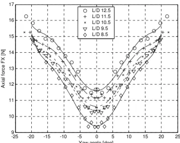
Page 2 of 6 and fins may be required to accommodate the propulsion and manoeuvring characteristics of the longer hulls. Figure 2 shows one of the models suspended from the PMM.
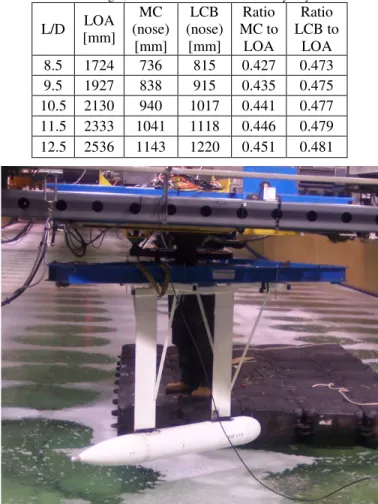
Table 1. Particulars of the five configurations tested; MC is the moment centre at the origin, LCB indicates the centre of buoyancy.
L/D LOA [mm] MC (nose) [mm] LCB (nose) [mm] Ratio MC to LOA Ratio LCB to LOA 8.5 1724 736 815 0.427 0.473 9.5 1927 838 915 0.435 0.475 10.5 2130 940 1017 0.441 0.477 11.5 2333 1041 1118 0.446 0.479 12.5 2536 1143 1220 0.451 0.481
IV. TEST PLAN
The test plan included the following runs for each of the five configurations.
a. straight-ahead resistance runs at various forward speeds - "resistance runs"
b. runs at constant forward speed with fixed yaw (drift)
angles - "static yaw runs"
c. pure sway runs with various combinations of amplitude and period - "pure sway runs"
d. pure yaw runs with various combinations of amplitude and period - "dynamic yaw runs"
e. arc-of-a-circle runs at constant tangential speed for various radii - "circular arc runs"
The test sequence was as follows. A particular configuration was assembled and was retained while the five sets of runs (a) to (e) were performed. Then the model was reconfigured and the same five sets of runs were repeated. In total over 197 runs were performed in a 10-day test period.
The straight-ahead resistance runs used fixed speeds of 1, 2, 3 and 4 m/s. The static yaw runs, the pure sway runs and the dynamic yaw runs were all performed at a single tow speed of 2 m/s. Initially all the circular arcs runs were to be performed at a constant tangential speed but hardware and software limitations prevented this; however certain combinations of tangential speed and arc radius were successfully employed. The set of completed runs is indicated in Table 2.
Table 2. Details of the test plan: number of runs performed.
L/D 8.5 9.5 10.5 11.5 12.5 Total Resistance 4 4 4 4 4 20 Static yaw 13 16 12 12 12 65 Pure sway 9 11 9 11 9 49 Dynamic yaw 11 6 7 5 5 34 Arc-of-a-circle 5 7 7 5 5 29 Total 197 V. DATA ANALYSIS
In the usual notation [2] the three orthogonal forces form a right-hand system with FX directed forward, FY directed to starboard and FZ directed toward the keel; see Fig 8. All the resistance runs were performed for zero drift angle, that is, with each model aligned with the direction of towing. The internal balance uses a single loadcell to measure the axial force FX directly, so FX is a direct measure of the hydrodynamic resistance experienced by the bare (un-appended) hull form. Thus the results can be presented directly in terms of curves of resistance [N] versus tow speed [m/s]. This balance uses two lateral-force loadcells to measure the total lateral force that the fluid exerts on the model. The total lateral force FY is obtained by summing the signals from these two loadcells. The total yaw moment MZ is computed about a vertical axis through a point whose axial location is mid-way between the two lateral-force loadcells which are 902 mm apart; the value of MZ is obtained by subtracting the signals from these two loadcells and multiplying the difference by one half of the distance between these loadcells.
All the static yaw runs were performed using a fixed sequence of yaw (drift) angles from -2 to +20 degrees in steps of two degrees. All runs were performed at a fixed speed of 2 m/s. The first step in the analysis was to plot the measured lateral force FY and yaw moment MZ versus yaw angle. Each curve was then shifted by a slight amount in order to provide
Figure 1. Schematic of the five configurations tested.
Page 3 of 6 zero yaw moment at zero yaw angle; this step accounts for the slight misalignment that occurs during model installation and zeroing of the PMM actuators. Next the data were reflected into the left half-plane. Finally, for each configuration, smooth curves were fitted of the form
y = a*β + b*β3
for the hydrodynamic loads that are odd functions of yaw angle 'β', here FY and MZ. Smooth curves of the form
y = a + b*β2 + c*β4 + d*β6
were fitted for loads that are even functions of yaw angle, here FX.
For the pure sway runs, the raw time-series data were filtered using the filtfilt function in MATLAB since this filter does not introduce any phase shift into the signal. Simple sinusoids were then fitted to the smoothed time-series using a least-squares technique. Time-series plots of the loads and sway velocity were created; these plots were used to extract the time interval by which each load lags the sway velocity.
VI. RESULTS
A. Resistance Runs
Figure 3 shows how the resistance (axial force) varies with tow speed and model length. The experimental data points are included in Figure 3 in order to show that the curves k*V^2 do in fact represent well the trends in the data. From this figure we can conclude that increasing the LDR from 8.5 to 12.5 results in an increase in resistance of 28 percent, at all speeds. Table 3 summarizes the results; R-square is included as a measure of goodness of fit..
Table 3. Curve-fit parameter 'k' for R = k*V2
L/D 8.5 9.5 10.5 11.5 12.5 k 2.11 2.13 2.41 2.55 2.71 R-sq 0.996 0.994 0.994 0.995 0.995
B. Static Yaw Runs
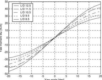
Figures 4, 5 and 6 show the hydrodynamic loads from the static yaw runs. The experimental data points are included in
Fig 4 in order to show that the fitted curves do in fact represent well the trends in the data. In the scale of Figures 5 and 6, it is not possible to discern the different experimental data points so they are omitted for clarity. The graphs for FX and MZ show distinct trends with increasing LDR. For the lateral force FY there appears to be only three curves since the curves for LDR of 9.5 and 10.5 appear to coincide, and, the curves for 11.5 and 12.5 appear to coincide. Figure 4 shows that the effect on FX of increasing the LDR is largest at zero yaw angle and this effect decreases as the yaw angle increases; as noted in Figure 3, increasing the LDR from 8.5 to 12.5 results in an increase in FX of 28 percent at zero yaw angle. For FY and MZ, Figures 5 and 6 respectively show that the effect of increasing the LDR is largest at the largest yaw angles, however it is clear that the slope of each curve (at the origin) increases with increasing LDR.
The results from the static yaw runs are summarized in Table 4. The values given in the row for FX are the minimum values, that is, the resistance at zero yaw angle for a speed of 2 m/s; these values can be used to compute the hydrodynamic coefficient 'Xuu' for each model length [2]. The values given in the row for FY are the slopes of the FY(β) curves at zero yaw angle; these values can be used to compute the hydrodynamic coefficient 'Yvv' for each model length. The values given in the row for MZ are the slopes of the MZ(β) curves at zero yaw angle; these values can be used to compute the hydrodynamic coefficient 'Nvv' for each model length.
Table 4. Some results from the static yaw runs for the five configurations at a forward speed of 2 m/s; minimum drag force at zero yaw angle and slopes for
FY and MZ at zero yaw angle.
L/D 8.5 9.5 10.5 11.5 12.5
Minimum drag force
[N] 9.4 10.3 10.6 11.2 11.6
Slope of lateral force
FY [N/deg] 3.14 3.26 3.46 3.87 3.87 Slope of yaw moment
MZ [N.m/deg] 1.89 2.13 2.41 2.84 3.02 0 0.5 1 1.5 2 2.5 3 3.5 4 0 5 10 15 20 25 30 35 40 45 Tow speed [m/s] D ra g f o rc e [ N ] k12 = 2.71 k11 = 2.55 k10 = 2.41 k9 = 2.13 k8 = 2.11 Values of k for R = k*(V2) L/D 12.5 L/D 11.5 L/D 10.5 L/D 9.5 L/D 8.5
Figure 3. Resistance versus tow force for the five configurations
-25 -20 -15 -10 -5 0 5 10 15 20 25 9 10 11 12 13 14 15 16 17
Yaw angle [deg]
A x ia l fo rc e F X [ N ] L/D 12.5 L/D 11.5 L/D 10.5 L/D 9.5 L/D 8.5
Page 4 of 6 Figure 7 shows the effect of increasing LDR at constant yaw angle for the yaw moment MZ. Six yaw angles were selected in order to portray this effect. Similar effects were observed for FX and FY but the graphs are not included here. From these curves it appears that all three loads FX, FY and MZ increase approximately linearly with LDR. For small yaw angles, the effect of increasing the model LDR from 8.5 to 12.5 is to increase FX by about 21 percent. For large yaw angles, where the effect of increasing the model LDR on FY and MZ is greatest; at a yaw angle of 20° FY and MZ increase by about 20 and 68 percent respectively as the LDR increases from 8.5 to 12.5.
C. Centre of Effort
In the same way that the "aerodynamic centre" for a 2D airfoil section can be found by searching for the axial location of an axis about which the pitching moment is zero, the axial location of a vertical axis about which the measured yaw moment MZ becomes zero can be found. Since the reported values of the measured MZ are about a vertical axis through
the origin (which is mid-way between the two lateral-force loadcells), the measured moment can be transferred to be about a vertical axis (which is forward of the origin 'O') at any other axial location as follows; see Figure 8. The moment transfer expression then becomes
MZ(x) = MZ(O) - FY(O)*x
where 'x' is measured positive forward of the origin, positive FY is to starboard and positive MZ has the nose of the vehicle swinging to starboard. Thus to find the axial location about which the measured yaw moment becomes zero, which we refer to as the centre of effort (COE), we have
x(MZ=0) = x(COE) = MZ(O) / FY(O).
Figure 9 shows how the axial location of the COE (ahead of the origin) varies with static yaw angle and LDR. As with the variation of FX with yaw angle, the largest effect on the COE of increasing the LDR is experienced at zero yaw angle. Near zero yaw angle, as a fraction of the overall length (LOA), the location of the COE moves aftward from about 0.35 of LOA to about 0.31 of LOA, as the LDR increases from 8.5 to 12.5. Since the CB is from 3 to 4.6 percent of LOA aft of the origin, at zero yaw angle the COE is about 0.40 of LOA ahead of the CB when the LDR is 8.5, and, is about 0.34 of LOA ahead of the CB when the LDR is 12.5. Thus the longest model, at zero yaw angle, as a fraction of overall length, has the COE which is closest to its CB.
D. Pure Sway Runs
Figure 10 shows a typical time-series for (i) the measured lateral force FY(t), and for (ii) the measured PMM sway velocity v(t), during a few cycles of steady-state motion, that
8.5 9 9.5 10 10.5 11 11.5 12 12.5 0 5 10 15 20 25 30 35 40 45 50
Hull length-to-diameter ratio
Y a w m o m e n t M Z [ N ] 0 deg 4 deg 8 deg 12 deg 16 deg 20 deg
Figure 7. Yaw moment MZ versus hull length-to-diameter ratio for various yaw angles for a tow speed of 2 m/s.
Figure 8. Diagram for the moment transfer - plan view
x, FX y FY O MZ(O) MZ(COE) = 0 x(COE) -20 -15 -10 -5 0 5 10 15 20 -150 -100 -50 0 50 100 150
Yaw angle [deg]
L a te ra l fo rc e F Y [ N ] L/D 12.5 L/D 11.5 L/D 10.5 L/D 9.5 L/D 8.5
Figure 5. Lateral force FY versus yaw angle for a tow speed of 2 m/s.
-20 -15 -10 -5 0 5 10 15 20 -50 -40 -30 -20 -10 0 10 20 30 40 50
Yaw angle [deg]
Y a w m o m e n t M Z [ N .m ] L/D 12.5 L/D 11.5 L/D 10.5 L/D 9.5 L/D 8.5
Page 5 of 6 is, once the motion has attained the required amplitude. Notice that the lateral force FY lags the sway velocity by about 2.31 seconds or 2.55 radians which corresponds to about 40 percent of one cycle of the motion.
Similar results were obtained for FY(t) for all the pure sway runs, regardless of the amplitude and period of the motion, and, model length. A similar behaviour was observed for the yaw moment MZ(t), that is, that MZ(t) lags the sway velocity v(t). Typical phase lags for FY(t) are shown in Table 5; these values are for one sway manoeuvre with amplitude 0.65 m and period 7.1 sec.
Table 5. Phase lag results for pure sway runs for the five configurations.
L/D Yo [m] To [s] Phi [rad] t(lag)/To
8.5 0.65 7.1 2.607 0.415
9.5 0.65 7.1 2.583 0.411
10.5 0.65 7.1 2.575 0.410
11.5 0.65 7.1 2.560 0.407
12.5 0.65 7.1 2.536 0.404
Phase-plane plots of FY(v) for the five model lengths are shown in Figure 11 and those for MZ(v) in Figure 12. Figures 11 and 12 and Table 5 show that the amount by which FY and MZ lag the sway velocity depends on the model length. These elliptical "trajectories" also show that neither FY nor MZ vary linearly with the sway velocity 'v'.
From the phase-plane plots two observations can be made: a. Higher-order, non-linear terms involving the sway velocity 'v' must be incorporated into the expressions for the hydrodynamic loads (in the equations of motion) in order to simulate correctly the hydrodynamic loads that are exerted on a bare hull during abrupt manoeuvres.
b. The phase lags between the sway velocity v(t) and the hydrodynamic loads FY(t) and MZ(t) depend on the LDR of the bare-hull. This relationship is depicted in Figure 13 for all the pure sway runs. The trends in all cases indicate that these phase lags decrease as the LDR of the hull increases. This
-20 -15 -10 -5 0 5 10 15 20 0.1 0.15 0.2 0.25 0.3 0.35
Yaw angle [deg]
A x ia l lo c a ti o n w h e re Y M i s z e ro , a s a f ra c ti o n o f L O A L/D 8.5 L/D 9.5 L/D 10.5 L/D 11.5 L/D 12.5
Figure 9. Axial location of the centre of effort as a function of yaw angle and length-to-diameter ratio.
65 70 75 80 85 90 -100 -50 0 50 100 Time [sec] L a te ra l fo rc e F Y [ N ] 65 70 75 80 85 90-0.6 -0.3 0 0.3 0.6 S w a y v e lo c it y [ m /s ] FY(t) v(t)
Figure 10. A typical time-series for the lateral force FY(t) and the PMM sway velocity v(t) during a few cycles of steady-state motion.
-0.6 -0.3 0 0.3 0.6 -150 -100 -50 0 50 100 150 Sway velocity [m/s] L a te ra l fo rc e F Y [ N ] L/D 8.5 L/D 9.5 L/D 10.5 L/D 11.5 L/D 12.5
Figure 11. Phase-plane plot of FY(v) for pure sway runs with amplitude 0.5 m and period 5.7 sec for the five configurations.
-0.6 -0.3 0 0.3 0.6 -50 -40 -30 -20 -10 0 10 20 30 40 50 Sway velocity [m/s] Y a w m o m e n t M Z [ N .m ] L/D 8.5 L/D 9.5 L/D 10.5 L/D 11.5 L/D 12.5
Figure 12. Phase-plane plot of MZ(v) for pure sway runs with amplitude 0.5 m and period 5.7 sec for the five configurations.
Page 6 of 6 relationship is not captured in the traditional expressions for the hydrodynamic loads that are exerted on a bare hull as a function of the sway velocity v(t).
Similar results were obtained from the dynamic yaw runs but due to space limitations the results are not shown here; those results will be published in a follow-up paper.
VII. CONCLUSIONS
During these experiments, the axial force FX, the lateral force FY and the yaw moment MZ were measured for a series of five models of the same diameter but of increasing length-to-diameter ratios of 8.5, 9.5, 10.5, 11.5 and 12.5. The increases in overall length were obtained by increasing the length of the constant-diameter mid-body by inserting pairs of equal-length spacers ahead and aft of the mid-body.
1. From the resistance experiments, it was shown that increasing the bare hull length-to-diameter ratio from 8.5 to 12.5 results in an increase in straight-ahead resistance of 28 percent, at all speeds.
2. From the static-yaw experiments, it was shown that: a. The FX(β) relation can be taken to be parabolic only for yaw angles 'β' less than about 7 degrees; above that angle both β4 and β6
terms are required in order to capture the effect of yaw angles up to 20 degrees. For a particular yaw angle, FX increases roughly linearly with an increase in the bare-hull length-to-diameter ratio.
b. The FY(β) and MZ(β) relations can be taken to be linear only for yaw angles 'β' less than about 7 degrees; above that angle a cubic term in 'β' is required in each relation in order to capture the effect of yaw angles up to 20 degrees. For a particular yaw angle, these loads increase roughly linearly with an increase in the bare-hull length-to-diameter ratio. 3. For the static yaw runs, useful values for FX, FY and MZ
are summarized in Table 4.
4. From the phase-plane plots of FY(v) and MZ(v) for the pure-sway runs, it was shown that two effects are present. a. Neither FY(v) nor MZ(v) vary linearly with the sway velocity 'v' during pure-sway runs. Thus higher-order, non-linear terms involving the sway velocity 'v' must be incorporated into the expressions for the hydrodynamic loads (in the equations of motion) in order to simulate correctly the hydrodynamic loads that are exerted on a bare hull during abrupt manoeuvres. Some expressions use terms in |v|v and v3 but further analysis is required to confirm whether or not such terms can model the measured effects adequately.
b. The phase lag between the sway velocity 'v' and the hydrodynamic loads FY(v) and MZ(v) depends on the bare-hull length-to-diameter ratio. The results of these experiments indicate that the phase lag decreases as the length-to-diameter ratio of the hull increases. This phase-lag relationship is not presently captured in the traditional expressions for the hydrodynamic loads that are exerted on a bare hull as a function of the sway velocity 'v'. For high-fidelity simulations of the behaviour of long, slender underwater vehicles, it will be necessary to incorporate such phase-lag relationships into the expressions for the hydrodynamic loads (in the equations of motion) that are exerted on a bare hull during abrupt manoeuvres.
5. For the pure sway runs, typical values for the amount by which the lateral force FY(t) lags the sway velocity v(t) can be found in Table 5, for a representative sway manoeuvre.
ACKNOWLEDGEMENTS
The authors would like to thank all the OCC and IOT staff and students for their assistance with this project. In particular we thank the facilities staff (towing tank, electronics, software engineering) for their enthusiasm and suggestions during the tests; all of that goes a long way to making the test period as productive as possible and ensures that the data are of high quality and value.
REFERENCES
[1] F.Azarsina, C.D.Williams and L.M.Lye, "Resistance and Static Yaw Experiments on the Underwater Vehicle "Phoenix"; Modeling and Analysis, Utilizing Statistical Design of Experiments Methodology", submitted to OCEANS'06 MTS/IEEE-Boston Conference, September 18 to 21, 2006, in press.
[2] J. Feldman, "DTNSRDC Revised Standard Submarine Equations of Motion", DTNSRDC report SPD-0393-09, June 1979.
For presentation at the Oceans'06 MTS/IEEE-Boston Conference, September 18 to 21, 2006
8.5 9.5 10.5 11.5 12.5 0.36 0.37 0.38 0.39 0.40 0.41 0.42 0.43 0.44
Hull length-to-diameter ratio
F Y l a g s s w a y v e lo c it y b y f ra c ti o n o f o n e c y c le Yo = 1.25m, T = 14.3s Yo = 0.90m, T = 9.5s Yo = 0.85m, T = 9.5s Yo = 0.70m, T = 14.3s Yo = 0.65m, T = 7.1s Yo = 0.50m, T = 5.7s Yo = 0.42m, T = 4.8s Yo = 0.36m, T = 4.1s Yo = 0.32m, T = 3.5s
Figure 13. Phase lag between lateral force FY(t) and sway velocity v(t) during all pure sway manoeuvres.