Boundary Element Modeling of Elasticity in
Materials
in
Terms of
Distribution
of
Second
Phase Structures
Yi Cheung Lok
B.Eng
.
Metallurgical Engineering McGill University, 200 1Submitted to the Department of Materials Science and Engineering on
May
18,2006 in partial fulfillment of the requirements for theDegree of Doctor of Philosophy
at the
Massachusetts Institute of Technology June 2006
O 2006 Massachusetts Institute of Technolog. All rights reserved.
MASSACHUSETTS INST~~VTE.~ OF TECHNOLOGY
1 I
JUL
1 9
2006
1 1
...
Signature of Author..
...
+ M ..
.-.
, .-1
~ e ~ m a t e r i a l s Science and EngineeringMay 15,2006
Certified by. .4.
...
.;p-...
--- ....
Adam
C.
Powell NAssistant Professor of Materials Science
and
Engineering Thesis Supervisor# n
/
.
0 . z.-.
.'.-.
Y. . x u . ..
:.
.
:.
.
.Y." .m.%.d.....
Accepted by..
...
Samuel Miller Allen POSCO Professor of Physical Metallurgy Chairman, Department Committee on Graduate Students
Boundary Element Modeling of Elasticity in
Materials in Terms of Distribution of Second Phase
Structures
YI CHEUNG LOK
Submitted to the Department of Materials Science and Engineering on May 18,2006 in partial fulfillment of the requirements for the Degree of Doctor of Science in Material Science and Engineering
ABSTRACT
The Boundary Element Method is used to study the interaction of second phase objects in a material. In particular, this study examines the relationship between stress parameters, such as stress concentration and normal traction, and geometrical parameters such as separation distance and orientation. The use of BEM enables easy manipulation of internal objects and rapid re-calculation in a series of simulations. Additional library functions are added to Julian, a general BEM solver, to expand its functionality to include elasticity calculation, inclusion modeling, and shape optimization with parallel processing. With a few thousand nodes, it is found that computation time scales as
o(N),
where N is the resolution of the mesh in each direction. An accuracy of over 99% is achieved in many benchmarks. A spherical cavity next to an inclusion is found to have higher stress concentration when aligned parallel to the loading direction. Stress analysis on a pair of neighboring cavities shows relatively small (less than 10%) increase in stress concentration beyond a separation of 0.5 diameter. While highest stress is observed when two cavities are aligned perpendicular to loading direction at very close separation, the highest stress configuration deviates from that alignment to almost+I-
30 degrees as separation increases. The radius of interaction is found to be determined by the larger of two second phase objects and is larger for a cavity surrounded by eight cavities in three dimensions. Our result suggests that a 15% weight saving is possible in a closed-cell foam for less than 10% increase in stress concentration due to the presence of immediate neighbors.Thesis Supervisor: Adam C. Powell IV
Acknowledgements
I would like to thank Adam C. Powell IV for being a great advisor. In an environment where the greatness of a faculty is often measured by impersonal statistic, he remains steadfast in his belief that education is first and foremost about the transfer of knowledge from the master to the apprentices. His dedication to undergraduate teaching is a testament to this belief. This dedication is only unmatched by that to his graduate students. The almost 2417 tech support, rapid and responsive email reply, flexible meeting schedule based on our need at the time, and last but not least, the effort to understand our progress and struggles are rare qualities that reflects his beliefs in the passing of wisdom to future generations and in treating others with respect and equality. His respect for his students is demonstrated by his willingness to consider other ideas and to accommodate the vastly different styles and personalities of his students. There will certainly be Julian with elasticity, but it might not have all the bells and whistles if not for the confidence he has in me and the freedom he entrusted upon me. This recognition of the uniqueness in each individual is the first and crucial step in bringing the best out of a person. Lastly, I would like to acknowledge his tireless effort in securing funding for my work. Over the past five years, there have been no less than five different sources of finding and only two TA assignments. Only with those supports shall we have the resources to make Julian worthy of the name it bears.
The following is a short list of family members and friends that I would like to thanks for their support over the years.
Q To my parents for their supports, encouragements and understandings.
*:* To Wendy for her patience, supports, encouragements and unwavering trust that turn
a grueling five-year long distance relationship into a rewarding experience.
*:* To my sister for her supports and her cynical view on the value of a PhD, which I shall prove her wrong.
*:
* To Lorna J. Gibson and Thomas W. Eagar, my committee members, for their
valuable advices on my thesis work as well as on my professional development. *:* To my two female group members, Bo and Wanida, for taking care of all the little
things in our office making it a pleasant working environment. *:
* Last but not least, to all my friends for keeping me distracted and busy for the past 4.5 year. Anything beats working in the office on a Friday night!
Table of Content
1 INTRODUCTION
...
9...
2 METHODOLOGY 13
...
2.1 THE BOUNDARY ELEMENT METHOD @EM) FORMULATION 14
...
2.1.1 Fundamental solution 15
...
2.1.2 Boundary Integral Equation 16
...
2.1.3 Discretization and evaluation of the Boundary Integral Equation 17...
2.2
ORGANIZATION
OF NODES IN JULIAN 18...
2.3 METHOD OF RIGID BODY DISPLACEMENT 19
...
2.4 SOLVING THE BOUNDARY INTEGRAL EQUATION 20
...
2.5 SETS AND RECALCULATION 20
...
2.6 INTERNAL STRESSES AND PRINCIPAL STRESSES 22
...
2.7 OPTIMIZATION AND PARALLEL PROCESSING 23
...
2.8 INCLUSION CALCULATIONS 24
3 RESULTS AND DISCUSSION
...
27...
3.1 BENCHMARKING JULIAN 27
...
3.1.1 Uniaxial tension 28
...
3.1.2 Uniaxial tension with spherical cavity 29
...
3.1.3 Uniaxial tension with two sphercal cavities 32
...
3.1.4 Uniaxial tension with spherical inclusion 35
...
3.1.5 Stress concentration on cavify and inclusion neara free surface
40....
3.1.6 Macroscopic stress and strain in the presence of carity and inclusion 49
...
3.2 CALCULATION TIME 51
...
3.2.1 Recalculation time 51
...
3.2.2 Break down of computation time by major components 53
...
3.3
MAXIMUM
NORMAL TRACTION ON A SPHERICAL INCLUSION 57...
3.4 INTERACTION BETWEEN TWO SECOND PHASE OBJECT 63
...
3.4.1 Interaction between two spherical cavities 63
...
3.4.2 Interaction between an inclusion and a cavify 69
...
3.5 INTERACTIONS BEYOND TWO SECOND PHASE OBJECTS 74
...
3.5.1 Nine cavities in a BCC arrangement 75
...
3.5.2 Nine inclusions in
a BCC arrangement
844 CONCLUSION
...
885 APPENDIX
...
93...
5.1 WEIGHTED RESIDUAL METHOD 93
...
5.2 CALCULAT~ON OF INTERNAL STRESSES AND PRINCIPAL STRESSES 96
5.3 SAMPLE PROGRAM USING JULIAN'S BEM LIBRARY FUNCTION FOR ELASTICITY
...
CALCULATION 101
...
List of Figures
Figure 3.1 - 1 Cylinder in uniaxial tension, color represents maximum principal stress .. . 2 8
Figure 3.1-2 Stress concentration on spherical cavity with 2000 simplex element, color
represents maximum z-stress ... 30
Figure 3.1-3 Stress concentration on two cavities with a/d = 0.3 ... 33
Figure 3.1-4 Stress concentration on two cavities with a/d = 0.9 ... 34
Figure 3.1-5 Spherical inclusion (2000 elements) inside the host material, color represent surface normal traction ... 36
Figure 3.1-6 Noda, N A . and Moriyama Y. (2004) analysis of stress state around a MnS inclusion in a high-strength steel matrix ... 37
Figure 3.1-7 Noda, MA. and Moriyama
Y
(2004) analysis of stress state around an A1203 inclusion in a high-strength steel matrix ... 38Figure 3.1-8 Comparison of maximum interface stress in high-strength steel matrix with an inclusion ... 39
Figure 3.1-9 Comparison of maximum normal traction on the inclusion in a uniaxially loaded high-strength steel matrix ... 39
Figure 3.1 - 10 Maximum principal stress on host material with an inclusion near a free surface . . . 4 1 Figure 3.1-1 1 Reproduction of a figure in Noda, N A . and Moriyama Y. (2004) showing the test setting o f a spherical inclusion in an semi-infinite body under uniaxial load.. . . . 44
Figure 3.1-12 Maximum principal stress on a cylinder with a cylindrical cavity in the center ... .. . . ... . . ... . .. . ... .. . ... . . . . . . . . . . . . . . . . . . . . 5 1 Figure 3.3-1 Maximum principal stress on inclusion with modulus ratio of 0.5, 1 and 2 (from left to right) ... 59
Figure 3.3-2 Normal traction on inclusion with modulus ratio of 0.5, 1 and 2 (from left to right) ... 59
Figure 3.4-1 Principal stress on a single cavity in a far-field uniaxial stress ... 66
Figure 3.4-2 Two spherical cavities at 20 degree showing the overlap region ... ... ... 67
Figure 3.4-3 Principal stress on two orbiting cavities at a separation of 0.1 diameter ... 69
Figure 3.4-4 Principal stress on an inclusion and an orbiting cavity at a separation of 3 cavity diameter.. . . 74
Figure 3.5- 1 Stress concentration on nine cavities in BCC arrangement (snapshots showing the xz-plane) ... 82
Figure 3.5-2 Principal stress on nine cavities in BCC arrangement (snapshots showing the xz-plane) ... 83
Figure 3.5-3 Maximum surface normal traction on nine inclusions in BCC arrangement (snapshots showing the xz-plane) ... 87
List of Graphs
Graph
3.1
- 1 Percent error as a function of defect resolution of a spherical cavi ty...... ...
3
1Graph
3.1-2
Interaction of Second Phase Objects with Free Surface as a Function of Separation...
48
Graph3.2-
1 Recalculation time as a function of the fraction of node recalculated...
53
Graph3.2-2
Calculation time as a function of mesh resolution on a1.4
GHz AMDOpteron processor
.
. .
. . .
.
. .
. .
.
. . .
. . .
.
. . .
. . .
.
. .
.
.
. . .
.
. . .
. .
.
. . .
. .
. . .
. . .
. . . .
.
. .
.
.
.
. .
5
5
Graph3.2-3
Distribution of total calculation time...
56
Graph3.3-1
Maximum Normal Traction and Principal Stressas
a Function of Young'sModulus Ratio
...
58
Graph3.3-2
Regression analysis of the maximum normal traction for modulus ratio c 1...
60
Graph3.3-3
Regression analysis of the maximum normal traction for modulus ratio > 1...
61
Graph3.3-4
Maximum normal tractionas
a function of Poisson's ratio...
62
Graph3.4-1
Maximum stress in loading direction on center cavity as a function oflocation of orbiting cavity for different separation distance in units of
diameter of cavity
...
. .. . . .
..
... . . .. ... .
. . .. . . .
. .
..
. . .
. . .
. . . .
. . . .
. . . .
. .
.
. . . .
.
65
Graph3.4-2
Percent Difference in Stress Concentration on Center Cavity as a Functionof Separation Distance Between Cavities at Different Angles
...
68
Graph3.4-3
Maximum principal stress on cavity as a function of location of orbitingcavity for different separation distance in units of diameter of cavity
..
...
...
70
Graph3.4-4
Stress concentration on cavity as a function of separation at different angles71
Graph
3.5-1
Relative difference in normalized principal stress and stress concentration versus separation between outer and center cavity...
77
Graph3.5-2
Relative difference in principal stress and stress in loading directioncompared to single cavity versus pore density
...
78
Graph
3.5-3
Comparison of stress concentration between the BCC arrangement and thecavity-cavity configuration at different angles
...
79
Graph
3.5-4
Variation in maximum normal traction on center inclusion and comerinclusion in BCC configuration versus separation distance
...
84
Graph3.5-5
Variation in surface normal traction with separation for two inclusionsList
of
Tables
...
Table 3.1.1 Benchmark for uniaxial tensile load on a cube and a cylinder 28
Table 3.1.2 Accuracy of spherical cavity with various different meshes ... 30
...
Table 3.1.3 Stress concentration on two neighboring spherical cavities 33
...
Table 3.1.4 Maximum normal traction on a "rigid" spherical inclusion 35
Table 3.1-5 Comparison of maximum normal tractions on an A1203 inclusion in a high-
...
strength steel matrix 38
Table 3.1-6 Comparison of maximum stress on the matrix interface in the loading
direction with a MnS inclusion in a high-strength steel matrix ... 38 Table 3.1-7 Stress concentration on 1000-element spherical cavity at distance b/d from
free surface ... 43 Table 3.1-8 Stress concentration on 2000-element spherical cavity at distance b/d from
free surface ... 43 Table 3.1-9 Stress concentration on 1350-element elliptical cavity at distance b/d from
free surface ... 43 Table 3.1-10 Maximum interface stress on 2000-elements spherical inclusion at distance
b/d from free surface ... 43 Table 3.1- 1 1 Maximum normal traction on 2000-elements spherical inclusion at distance
...
b/d from free surface 44
...
Chapter 1
Introduction
Stress distribution around cavities and inclusions has been studied by many investigators in the past 80 years. In particular, the stress concentration factor of a feature in a component is an important consideration in mechanical design, which gives the local stress compared to the applied stress. However, it is not a useful measure in fracture mechanics because stress concentration at crack tip is infinite; hence another parameter, the stress intensity factor, is defined for describing stress around crack tip. Although stress concentration factor cannot directly estimate the amount of applied stress required for crack propagation, it can predict the probability of such event at a given location. This is because the amplified external stress in regions of high stress concentration adds to that around any existing flaws.
Without modern computational tools, early investigators often attempted to derive analytical solutions for very specific arrangements of defects, limited by the complexity of the mathematics involved. With the advent of computer and stress analysis software, such as the many commercial Finite Element Method (FEM) packages, the need to derive a general solution for any particular arrangement might now seem superfluous. An engineer can perform a FEM analysis and obtain the stress distribution in a matter of hours if not minutes. Therefore, it is not the focus of this study to determine the stress concentration value for any particular defect arrangement. Instead, the focus of this study
is centered on the relationship between stress concentration and relevant geometrical and
materials parameters.
This type of relationship is most evident in a closed-form analytical solution. For
example, the stress concentration factor of an elliptical notch in an semi-infinite plate is
given by the relatively simple expression, k, = 1
+
2t
- . It is clear from the expression that stress concentration is linearly proportional to the square root of t/r, where t is thedepth of the notch and r is the tip radius. Understanding this relationship, an engineer
knows that if the design calls for a deeper notch, the radius of the notch must also
increase by the same factor to avoid a raise in stress concentration. In addition, because
of the square root relationship, an engineer's decision to vary the t/r ratio could be depend
on its value.
Similarly, a materials engineer on the assembly floor might be performing an x-
ray inspection and notice a cluster of cavities in close proximity. Without the access to or
the time for simulation, the engineer needs to make a quick decision and decide whether
the component should be reworked. He or she will be able to make informed decisions
based on a good understanding of how stress concentration varies with separation.
Unfortunately, closed-form analytical solutions are only available for the simplest of
situations such as a single cavity in an infinite medium. Analytical solutions have been
proposed for more complex problems such as two spherical cavities in an infinite region
[12], but the resulting infinite series solution is far from trivial. Normally, when an
relationships between measurable parameters. It is thus the objective of this study to examine those relationships and ultimately enhance our understanding of the interaction of second phase objects using data produced by numerical simulations. The motivation of this work is captured in words by Peterson [lo] in the preface to his book: ". . . to achieve better balanced designs of structures and machines - conserving material, obtaining cost reduction, and achieving lighter and more efficient apparatus".
As mentioned above, the problem of stress distribution around defects has been studied by many investigators in the past. The body of work on the subject over the past century is too numerous to be listed here. Some of those results will be cited for comparison where appropriate in later chapters. Peterson [lo] has compiled together an extensive reference of work done in this subject area. Of particular mention is the Boundary Element Method (BEM) work of Zhenhan Yao's group at Tsinghua University. They have published a paper on BEM modeling of inclusions in as early as 2002. Their 2003 paper [16] provided insights for the implementation of inclusion calculation in Julian, an open source BEM solver. A 2-D result with 100 inclusions is presented in that paper. In their recent 2004 paper [17], they claimed to have the ability to model as many
as 1600 inclusions in 2-D using the multipole BEM technique proposed by Greengard L.
and Rokhlin V. [5].
The remainder of this thesis consists of two major sections. Chapter Chapter 2 explains the methodologies used in this study. This includes a general overview of the Boundary Element Method as well as some of the more unique features of Julian such as
the concept of sets, recalculation of modified sets, inclusion calculation, and shape optimization using parallel processing. The purpose of the chapter is to explain how Julian is specially designed to efficiently study the interaction of second phase objects in materials. Results of our simulations are presented in Chapter Chapter 3. The first portion of the chapter compares Julian's calculation result with analytical solutions if available or results from other investigators. This is followed by a discussion of computation time, an important consideration in any numerical simulation. It demonstrates Julian's efficiency in performing iterative calculations. The rest of chapter Chapter 3 examines the effect on stress concentration of parameters such as Young's modulus ratio Eind/Ehost, separation
Chapter
2
Methodology
The objective of this study is to investigate the interaction of second phase objects and obtain relationships between relevant measurable parameters. The most popular method for stress analysis in solids is the Finite Element Method (FEM). Some of its popularity can be attributed to its versatility and efficiency. For a large, complex 3-D mesh, FEM is more efficient than BEM in both computation time and memory usage. However, BEM offers one advantage over FEM, which is a simpler meshing
requirement. While FEM requires a volumetric mesh in a
3-D
model, BEM demands onlya surface mesh.
The benefit is hardly noticeable in applications where mesh generation is only done once in the beginning. However, this becomes an attractive feature in situations where the mesh needs to be regenerated many times over the course of a simulation. This is especially true for the modeling of internal features such as cavities and inclusions. For example, to model a second phase object at various locations inside a component using BEM, one needs only translate the defect portion of the mesh. Because the rest of the mesh is not modified in any way, the corresponding matrix can be reused in the new calculation. The details of this process will be explained in Section 2.5. The same applies to rotation, dilation or a combination of such operations on internal features.
Sandgren, E. & Wu, S.J. [12] pointed out in the context of shape optimization using BEM that the minor modification to the mesh in the case of BEM versus complete
mesh regeneration in FEM gives a greater confidence that the changes observed in
measured parameters such as stress concentration are not affected by the difference in
accuracy due to remeshing. In the study of stress concentration and normal traction where
the accuracy for stresses on the surface is crucial, BEM is also believed to produce a
more accurate boundary stress than FEM [8].
2.7 The Boundary Element Method (BEM) formulation
The 2-D elasticity formulation of the boundary element integral method was proposed by Frank Rizzo in a paper published in 1967 [ l l ] . The generalized 3-D
elasticity formulation was published two years later in a paper by Cruse, TA. [2]. The governing elasticity equation used in BEM is the same as the one used in FEM, namely
the Navier-Cauchy equations of equilibrium
A m 2 0 ( x i + ( X + G ) v [ v e s ( z ) ] + 3 = A i)
Equation 2- 1 Navier-Cauchy Equation where G is the shear modulus, D(Z) is the displacement vector, /Z is one of the Lame
U L constants given by X =
[(I
+
v ) (1 - 2v)] ' is a vector representing body forces andE and v are Young's modulus and Poisson's ratio respectively. The BEM formulation for
linear elasticity can be derived using several approaches. Derivation using Betti's
employing the method of weighted residuals is given in Cartwright, D. [I]. An outline of that derivation is given in the Appendix (see Section 5.1).
2.1
.I
Fundamental solutionThe Navier-Cauchy equation (Equation 2-1) can be expressed in component form as Guk,j
( x )
+
(A
+
G) u,,,,
( x )
+
bk( x )
= 0v,
k = 1,2,3). The fundamental solution for this equation was derived in the late 19" century by William Thomson (Lord Kelvin). The solution gives the response in displacement field uj at point q due to a unit point force ejat point p in an infinitely extended three-dimensional elastic solid
Equation 2-2 Fundamental solution to Navier Equation where
Equation 2-3 Kernel function Qj Using the generalized Hooke's Law, one can relate the displacement field to stresses, which can then be expressed in tractions t at point q on a given plane with an outward normal n.
t j ( q ) = q(q9 P ) ~ , ( P )
Equation 2-4 Traction response due to unit point load
-1
[(I - 2 4 (nj=j - nj=j)
+
(3cj=j+
(1 - 20) 60) nmcm]Equation 2-5 Kernel function TI
2.1.2 Boundary Integral Equation
The defining characteristic of BEM is a mesh-free interior. This requires that the entire state of the system be defined using solely values on the boundary. This characteristic is reflected in the weighted residual statement for BEM, derived using the weighted residual method (see Section 5. I),
Equation 2-6 Simplified weighted residual statement where
4
(x,) and tj are displacement and traction respectively;U!,
and5
are the kernel functions as defined in previous section.Notice that apart from the body force term, the displacement at any interior point p within the boundary S, iij (x,) , can now be calculated just by evaluating the surface integrals on the boundary. The body force term is often known a priori and can be evaluated independently. The unknown boundary conditions can be evaluated by letting the interior point p approaches boundary points q. However, this leads to a singularity in the traction kernel function
z'
when x, = xq; as a result, an additional term cg is necessary to account for that singularity and to allow the integral$ 5
(
x ,, x,)
u
(
x q ) dS to be evaluated as theS
Cauchy principal value. The hat above ul and
tJ
will be left out in favor of a simpler notation. The boundary integral equation can then be rewritten asS
Equation 2-7 Boundary integral equation
2.1.3 Discretization and evaluation of the Boundary Integral Equation
The surface integral must be discretized into elements composed of nodes to be modeled numerically using ~ulian'. The discretized version of the boundary integral equations is
Equation 2-8 Discretized boundary integral equation where
Equation 2-9 Gij
e
Equation 2-10 Hii Note the difference in superscripts on
C,
ff
and4,
P. While
4
and P correspond to the nodal value of displacement and traction hence the a superscript,C
andff
are integrals of the kernel functions4
andzl
evaluated over the element & hence the e superscript. The introduction of shape function Nu allows the displacement and traction variables betaken outside of the integral. Julian calculates this integral over the element using the Gauss-Legendre Integration. An example of Gauss-Legendre Integration for the kernel function GIJ is given below.
-I Julian is a set of open source library functions for BEM calculations. It is being developed by Prof.
kl=l k -1
-
2- Weights given to fcn evaluated at each ordinate pointsKernel function. evaluated at n ordinate points for each elemental node x
.
inter- polating to give globafvalueor the element
--
Shape function. Jacobian, scale governs inter- global to intrinsic polation of coordinate nodal valuesThe evaluation of the
4
integral is slightly different from the above formulation (Equation 2-1) in Julian. The unit normal nk is factored out of thez,
function and ismultiplied with the kernel function during integration; i.e.
2.2
Organization of nodes in Julian
The double summation in the discretized boundary integral equation aims to calculate the sum of GutJ and Hguj values over all the nodes on the boundary. This is done
by first calculating a "per element" total by summing over the number of nodes per element M in the inner summation, then the per element total from all the elements
N'
are added together. In other words, the nodes are organized into two levels, the element level and the node level. In Julian, the nodes are organized into four levels. The nodes are first organized in sets and within each set there can be numerous element groups. Each groupis composed of many elements and each element is composed of a certain number of nodes. The organization into sets is a convenient way to group a set of related nodes, such as nodes belonging to a defect or a series of defects. The advantage of grouping into sets
should be more apparent in subsequent discussion on Sets and Recalculation (see Section 2.5). Within each set, the nodes are organized into element groups by the different boundary conditions. On the element group level, Julian follows the discretized boundary integral equation.
2.3
Method of Rigid Body Displacement
The discretized boundary integral equation can be written in matrix equivalents, namely
Equation 2-1 1 Boundary integral equation in matrix notation Notice that the [c] matrix is now part of the [HI matrix. Evaluation of the [c] matrix analytically is rather complex, especially for corner nodes. It should be reminded that the [c] matrix is created to allow the singularity in the diagonals (when
x,
=x,)
of the [HI matrix be evaluated directly. Luckily the diagonals can be evaluated indirectly as is done in Julian, avoiding the singularity, by a technique called rigid body displacement. In this technique, a finite body is subject to a unit rigid body displacement while the surface traction must all be zero. The resulting boundary integral equation is [HI {I) = [GI {0) = (0) , where(0
is a column vector of unit displacement in a particular Cartesian direction. It is therefore obvious that the diagonal value of the[HI
matrix is equal to the negative sum of all the non-diagonal values in that Cartesian direction,N
namely [ H I ; = ( & - I ) ~ [ H ] ; . m=l
2.4
Solving the Boundary Integral Equation
Boundary conditions usually consist of a mixture of traction (Neumann) and displacement (Dirichlet) boundary conditions. It should be noted that for the problem to have a unique solution, exactly half of the boundary conditions must be specified. In that case, each of the { u } and
{t}
vector is composed of both known and unknown values. In order to solve the matrix efficiently using matrix algebra, it is thus necessary to isolate all the unknowns in one vector. In Julian, the equation[HI
{u} =[G]{t}
is transformed into[ A ]
{x}
=[B]
{y} , where theW
vector contains all the known boundary conditions while the {x} vector becomes the unknown vector. Rows are swapped between the { u } and {t}vector to create the
{x}
andCy}
vector; similarly, the corresponding columns should be swapped between the[HJ
and[a
matrix resulting in the [A] and[a
matrix. This information is recorded so that the boundary conditions can be swapped back to their original positions after the calculation. After calculating the matrix multiplication[a
Cy),
Julian solves the unknown vector{x}
by performing the Doolittle decomposition. a version of LU decomposition that has a unit lower triangular matrix, on the[A]
matrix. Partial pivoting is used in the decomposition process to avoid potential instability.2.5
Sets and recalculation
Earlier in the discussion, in Section 2.2, the notion of sets was briefly introduced. It was explained that nodes belonging to similar structural features such as an internal defect are grouped together in a set. The main benefit of this arrangement is to facilitate the recalculation of those nodes belonging to a particular structural feature, for instance to
evaluate the mechanical response of a casting as an internal cavity moves from one location to another. If this were to be done in FEM, it would most likely require a rebuilding of most of the mesh, which means having to recalculate everything from scratch. For BEM, since the internal cavity is not linked to any other portion of the structure by an interior mesh, it is thus possible to move an enclosed section of mesh while keeping others intact. This is not to say that the mechanical response for the intact portion of the structure need not be recalculated; yet the solution time is greatly reduced during recalculation. The two most computation expensive procedures in Julian's BEM calculation are the building of the
[HI
and[GI
matrices as well as the LU decomposition of the [A] matrix. From earlier discussion,fi,
and Gy are given by the following integral(Equation 2-9, Equation 2-10)
G; (xq , xp) =
J
ug
(xq , xp) N, (xq) (x,) r eH; (x, , xp) =
$
q
(x, 9 xp) N, (x,) (x,) ' r eIt should be rather obvious that
fi,
and Gg is not a function of any other variables besidesx, and the ordinate points x, for the Gaussian integration within the element. Therefore the addition of extra boundaries such as an internal cavity to the system results only in an expanded matrix and the existing values within the matrix remains intact. Similarly, modifying the coordinates of existing nodes requires changes in the rows and columns in the
[a
and [GI matrix associated with those modified nodes. Note that the changes do not affect the values offi,
and Gy in sets prior to the set containing the modified nodes. The following drawing illustrates how the entire[a
or[GI
matrix is partitioned into regions after two more sets are added to the original matrix. Usually, set 0 is comprisedof the external boundary of a component and internal objects such as cavities are assigned to the additional sets.
[ i ; i ; i ; i ; i ; i ; i : i : i : i ; i ; i ; i ; j Set 0
I
Set 1Set 2
A LU decomposed [A] matrix can be used repeatedly to solve the
equation [ A ] { x } = [ B ] { y } . However, since LU decomposition uses numbers from previous sets to calculate the current set, changing the values in one set once again requires only subsequent sets be decomposed again.
2.6
Internal stresses and principal stresses
Julian's BEM solver returns the result in the form of displacements and tractions in the Cartesian directions for all boundary nodes. A post-processing procedure calculates the complete stress state as well as the principal stresses, the Tresca and the Von Mises stresses, and the normal traction. The method used in Julian follows closely the steps outlined in Gao,
X
andDavis,
T [4]. An outline of that calculation is given the Appendix2.7
Optimization and parallel processing
The development of optimization in Julian is currently at an initial stage. The algorithm performs an unconstrained optimization of a specific stress component on an internal object by varying its location within a host. The target stress component is sampled at six different locations around the initial position, two in each directions. The slopes of the gradients are calculated and a new location is estimated using Newton's method.
One of the major challenges is to develop an optimization code that is efficient and yet general enough to work with any geometry without a user defined boundary. For example, by using a small step size, the increase in stress on a cavity as it approaches a wall or another internal object acts as a natural boundary. On the other hand, the downside of using small step size is inefficiency and a greater probability of getting caught in a local minimum.
Optimization in Julian is broken down into parent and child processes. A single parent process is responsible for calculating stresses at the actual location of the object, spawning new child processes to calculate stresses at neighboring locations, and integrating results generated by the children. The parent process is also where the optimization algorithm is located. The sampling of the target stress component around the actual location is handled by a network of computers. Each child process is responsible for evaluating the two sample points in one of the three orthogonal directions. Using this configuration, three processors are required for each object to be optimized. In a large
problem, the transfer of the decomposed and swapped
[M
and[q
matrices from parent to child can be a time consuming task if the child process runs on a different machine. As a result, there are only limited benefits in using more processors per object. In addition, one should reconsider the benefit of transferring the matrices if it takes more time than it saves in recalculation.2.8
inclusion calculations
Elasticity calculation of inclusion using BEM in
2-D
has been demonstrated in a paper by Yao, 2. et al. [16]. Julian adopted a similar approach. The stress state around an inclusion is analyzed by considering a hole in the host material that is being filled by a material with different mechanical properties. The cavity in the matrix has its displacement and traction coupled to a similarly sized, shaped and meshed material of different Young's modulus and Poisson's ratio. At the inclusion/matrix interface, the displacements in the inclusion and the matrix are assumed to be equal, and the traction is assumed to be equal and opposite. In terms of linear algebra, recall we have for the host material1
set
Yt1
2]
s e t } =[
~ f i ~ ~ ]
{
'set1}
H ; ; ~ uset, Ggt2 G;F2 tset2where superscript set 1 and 2 denotes the portion of the matrix responsible for the calculation of the host and the cavity. In situations where we only interested in calculating stress around cavity, zero traction = 0 is the prescribed boundary condition. In the case of inclusion calculation, since both traction and displacement are non-zero and are in fact coupled to the inclusion, an extra set of equation is needed to
solve the above system of equations. A similar [&*cl.] { ~ j n ~ l . } = [ G ~ ~ ~ ~ . ] {tinCl.} matrix equation can be constructed for the inclusion. Once again, none of the boundary conditions in the inclusion matrix equation is known a-priori. Isolating tincl., the above expression becomes
Equation 2-1 2 Surface traction on inclusion Since the traction on the cavity is equal but opposite to that on the inclusion, the traction expression to be back substituted into the host material should therefore be
'set 2 = - = -
[
Gincl.1-
'
[
H i n c ~ .]
{
uincl.)
Note that [HI,
[a,
{u} and {t} are replaced by [A], [B], {u} and {t} to be consistent with earlier notation highlighting the fact that the boundary conditions are now swapped into the unknown {x} and known0
.
1
vectors. Since ujnCl = usetz, the displacement on the cavity can be grouped together as47'
4:t2
4Yt2
Yset 1[ G ~ ~
4;t2]
{
Zl
}
=[
B ~ F ~';it2]
[-
[GjnClj-l [HjnclI{
uset21
1
Equation 2-13 Modified boundary integral equation for inclusion calculation Julian follows this approach but instead of truncating the [B] and {y} matrices, it keeps the two matrices intact because ysetz has zero values by default for cavity. Upon calculating usetz, traction on the inclusion can be calculated using Equation 2-1 2.
In the calculation for the [Hj and
[4
matrices of the inclusion, note that since the kernel functionsul
(Equation 2-3) and (Equation 2-5) are functions ofr,
separation between field point and source point, the actual location of the inclusion in the parent becomes unimportant. However, extra care must be taken to ensure the inclusion has the same size as the cavity for r is directly related to separation between node points. It should also be obvious that since the result of the inclusion calculation is back substituted into that of the host material, the inclusion and the cavity in the host must have the same mesh. The only difference is the orientation of the surface normal, where the cavity has inward surface normal and the inclusion has outward surface normal.Chapter 3
Results and discussion
This chapter presents some of the simulation results. Various benchmark tests are conducted to demonstrate Julian's capabilities and limits as well as the quality of its result. These benchmark results are covered in Section 3.1. Section 3.2 shows the result of a series of timed runs. It demonstrates the efficiency of using matrix sets and
BEM
in iterative type calculation. The relationship between the Ehdcl/Em,m, ratio and themaximum normal traction is presented in Section 3.3. Section 3.4 examines the interactions between two spherical cavities and that between a spherical inclusion and cavity respectively. A case study of a non-random distribution of nine cavities and nine inclusions are analyzed in Section 3.5. The nine cavities and inclusions are positioned in a BCC arrangement. Important parameters such as stress concentration and normal traction are evaluated as a function of the separation between them.
3.7
Benchmarking Julian
A series of tests are conducted to validate the accuracy of Julian in elasticity calculation and in particular, materials with a cavity and an inclusion. As mentioned in previous chapter, Julian is capable of computing the complete stress state on all external and internal surfaces.
3.1
.I
Uniaxial tensionUniaxial tension tests are performed on a 20 unit x 20 unit x20 unit cube and a cylinder with a radius of 5 units and a length of 10 units. The objectives of these two uniaxial tension tests are: first, to demonstrate Julian's accuracy in estimating stress and strain under uniaxial load on two simple geometries and second, to estimate the inherent error
in the mesh of these two geometries which will be used in most of subsequent tests. The Young's modulus used in the simulation is 200GPa and the Poisson ratio used is 0.3 and 0 for the cube and the cylinder respectively.
Table 3.1-1 Benchmark for uniaxial tensile load on a cube and a cylinder
Figure 3.1-1 Cylinder in uniaxial tension, color represents maximum principal stress
% Error 0.02% 1.29% Simulation Stress (Pa) 1000 1700 20258700 Applied Displacement 0.00 1 0.001 Mesh Geometry Cube Cylinder Theoretical Stress (Pa) 10000000 20000000 Number of Elements 432 420
The simulation stress given in the table above is an average value of all elements on the surface where the displacement is applied. As the result shows, the simulated value is in good agreement with theoretical predictions, with negligible error in the cube case and an error of slightly above 1% in the cylinder case.
3.1.2 Uniaxial tension with spherical cavity
The following results compare the value calculated by Julian to the theoretical value for stress concentration on a spherical cavity when a rectangular bar containing that cavity is subjected to a uniformly applied tensile stress. When the loading is uniaxial tension in the z-direction, the theoretical maximum stress on the spherical cavity is outlined in
Timoshenko S. P. and Goodier J. N [15] as
where ( o ~ ) ~ , is the maximum stress in the z-direction, v is the Poisson's ratio, and S is the magnitude of the applied stress. The stress concentration factor k, can be calculated from the above equation
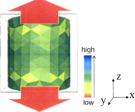
Equation 3-1 Stress concentration factor on a spherical cavity in an i&nite body The dimension of the block is 20x20~20 and the radius of the spherical cavity is 0.5 (see Figure 3.1-2). Aside from the resolution of the cavity, all simulation parameters are identical in all of the tests. The block has a Young's modulus of 200GPa and a Poisson's Ratio of 0.3. The results are summarized in the following table.
Table 3.1-2 Accuracy of spherical cavity with various different meshes
Figure 3.1-2 Stress concentration on spherical cavity with 2000 simplex element, color represents maximum z-stress
high
I
-1
# of Elements 1 00 500 1000 2000 100 450 Theoretical Stress Concentration 2.05 2.05 2.05 2.05 2.05 2.05 % Error 8.78% 2.43% 0.94% 0.55% 3.28% 0.51 % Element Type Linear Linear Linear Linear Parabolic Parabolic Stress Concentration 1.87 2 .OO 2.03 2.03 1.98 2.04Graph 3.1-1 Percent error as a function of defect resolution of a spherical cavity
500 1000 1500 2000
Number of linear simplex element in spherical cavity
In general, the simulation result tends to underestimate the actual stress concentration, a result of the mesh's imperfect representation of a sphere. It is very important to keep that in mind when using Julian to perform stress analysis since underestimation of that nature can lead to overly optimistic conclusions. It is obvious from Graph 3.1-1 that as the number of elements on the spherical cavity increases the accuracy is improved as well. Notice that the curves in Graph 3.1-1 are highly non-linear and appear to flatten out above 1000 elements. Since the solution time of BEM goes as the 6 power of the resolution of a mesh, the additional computation cost clearly outweighs the little benefit in improved accuracy by going over 1000 elements for a spherical cavity. Therefore, the mesh with 1000 simplex elements is chosen to be used unless otherwise specified, in all
our tests because it provides a good compromise between accuracy and computation time.
Two types of element are used in these tests, namely simplex and parabolic. The simplex element used here is a linear triangular element with three nodes, one at each of the corners. The parabolic element being used is similar to the simplex element, but instead of having straight lines connecting the three corners a parabolic curve is used. As a result, a parabolic element has three more nodes in-between the corners hence a total of six nodes per element. Therefore as one might expect, a parabolic element is better suited for meshing a curved surface such as a sphere. This is shown clearly in the result (see Table 3.1-2) where a spherical mesh using 450 parabolic elements achieves roughly the same accuracy of about 0.5% with less than a quarter of the number of elements needed by a mesh with simplex elements (2000 elements). However the saving in elements required does not translate into any noticeable gain in computation time when using a parabolic mesh that has fewer elements for a given accuracy level. This is probably due to the higher node counts in each parabolic element compared to a simplex element.
3.1.3 Uniaxial tension with two spherical cavities
Noda, MA. and Moriyama Y. [9] has calculated stress concentration on two spherical cavities in close proximity to each other using the body force method with singular integral equations. Similar simulations are conducted using Julian and the results are compared with Noda's calculation. The material used in the simulation has a Young's modulus of 200GPa and a Poisson's ratio of 0.3. Once again the two cavities are housed
inside a 20x20~20 cube uniaxially loaded in the z-direction. The radius of the spherical cavity is 0.5. In all of the tests, the wall of the cavity and the wall of the cube have a clearance of at least seven diameters to ensure minimal interactions. The following table summarizes the result.
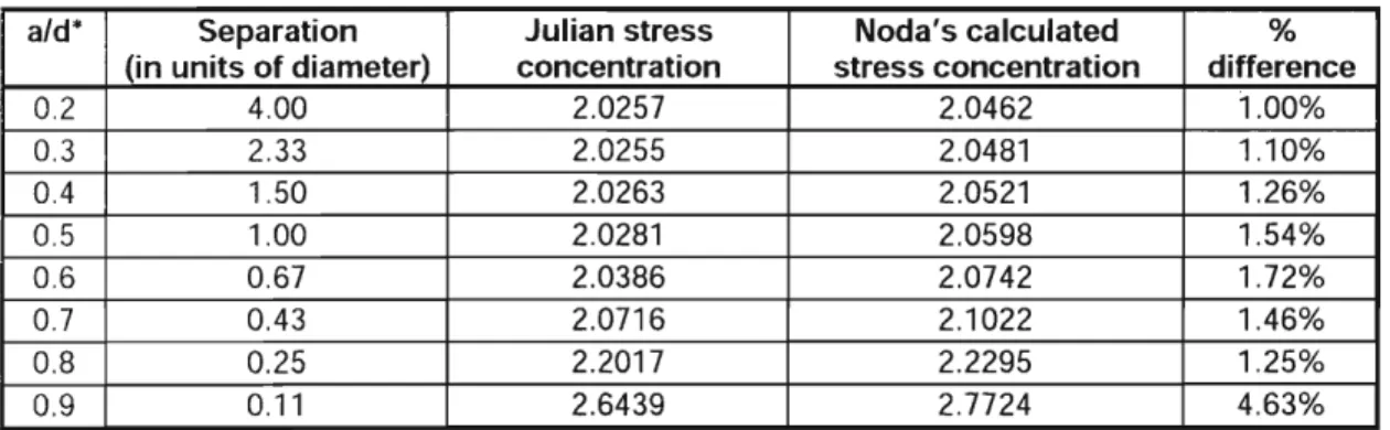
Table 3.1-3 Stress concentration on two neighboring spherical cavities
I
a/daI
SeparationI
Julian stressI
Noda's calculatedI
%I
*a is the radius of a cavity and 2d is the center-to-center separation between the cavities (see Figure 3.1-3) Figure 3.1-3 Stress concentration on two cavities with a/d = 0.3
0.2
(in units of diameter) 4.00 concentration 2.0257 stress concentration 2.0462 difference i
.oo%
Figure 3.1-4 Stress concentration on two cavities with a/d = 0.9
hiqh
.
,I m
low
To be consistent with Noda's notation, the simulations are run at various a/d values, where a is the radius for a spherical cavity and 2d is the center to center separation between the two cavities (see Figure 3.1-3). The second column gives the wall-to-wall
separation between the two spheres in units of diameter. The difference between Julian's result and that of Noda varies between 1-2%. Given that the spherical mesh used as cavity has an inherent error of 0.94%' the simulation result seems to be in good
agreement with Noda's calculation. The two results begin to diverge when a/d equals 0.9 (Figure 3.1-4), which is equivalent to a wall-to-wall separation of 11% the diameter of the cavity likely because of insufficient mesh resolution. At the opposite end of the a/d
range, at a separation of 4 times the diameter (a/d = 0.2), the stress concentration on the
3.1.4 Uniaxial tension with spherical inclusion
The analytical solution for stress field around a rigid spherical inclusion, i.e. = oo , has been derived by
Goodier,
J N [5]. The expression for the maximum EmatrIxadhesion stress at the pole position is given by
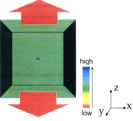
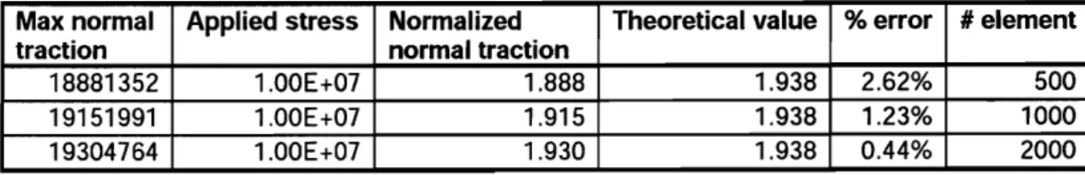
Equation 3-2 Maximum adhesion stress on a rigid spherical inclusion in an idnite body For v = 0.3, the maximum traction on a rigid spherical inclusion given by the above equation is 1.938. A perfectly rigid inclusion is not a realistic condition in numerical modeling; therefore the condition is approximated by having an inclusion that is 1000 times more rigid than the matrix. The simulation is conducted in a similar fashion to previous benchmark tests. An inclusion with radius of 0.5 is located in the center of a 20x20~20 cube loaded uniaxially (see Figure 3.1-5). The host material has a Young's modulus of 200GPa and a Poisson's ratio of 0.3; the inclusion has a Young's modulus of 200TPa and a Poisson's ratio of 0.3. Two simulations are performed under the same conditions using spherical meshes with different number of elements for the inclusion. The result is summarized in the following table.
Table 3.1-4 Maximum normal traction on a "rigid" spherical inclusion
# element 500 1000 2000 % error 2.62% 1.23% 0.44% Theoretical value 1.938 1.938 1.938 Max normal traction 18881 352 191 51 991 19304764 Applied stress 1.00E+07 1.00E+07 1.00E+07 Normalized normal traction 1.888 1.91 5 1.930
Figure 3.1-5 Spherical inclusion (2000 elements) inside the host material,
color represent surface normal traction
m
high
low
As in the cavity case, the simulation underestimates the maximum normal traction. However in this case, part of that underestimation can be attributed to the approximation
of a perfectly rigid inclusion. The result shows a slightly larger error in the 1000-element mesh when it is being used as an inclusion as opposed to as a cavity. On the other hand, it is quite surprising that the 2000-element mesh does a little better in the inclusion test than in the cavity test. Overall, despite having to approximate a rigid inclusion, Julian's result matches well with theoretical values to within 3% even with the relatively coarse 500- element mesh. The relationship between the Ejncl,/Ematriu ratio and the maximum normal traction will be discussed in Section 3.3.
Since Goodier's work in 1933, other researchers have developed ways to calculate stress states around inclusions for any &nd./Ematrix ratio. Using the same method as in the
two spherical cavities calculation, Noda, NA. and Moriyama
Y
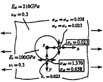
[9] analyzed the stress state around a spherical inclusion in a uniaxially loaded infinite body. Two different materials for inclusion in a high-strength steel matrix were evaluated. The first type is a MnS inclusion with roughly half the Young's modulus of high-strength steel; whereas the second one is an Alz03 inclusion that has about twice the Young's modulus of the matrix. The result of that analysis from their 2004 paper is reproduced here in the following two figures.Figure 3.1-6 Noda, h? A. and Moriyama K (2004) analysis of stress state around a MnS inclusion in a high- strength steel matrix
Figure 3.1-7 Noda, N.A. and Moziyama K ((2004) analysis of stress state around an A1203 inclusion in a high-strength steel matrix
A similar analysis was conducted using Julian. An inclusion with radius of 0.5 is located
in the center of a 20x20~20 cube loaded uniaxially with Young's modulus of 210GPa and
a Poisson's ratio of 0.3. In the MnS case, the inclusion has a Young's modulus of lOOGPa and a Poisson's ratio of 0.3; whereas, in the Al2O3 test, the inclusion has a Young's modulus of 400GPa and a Poisson's ratio of 0.25. Julian's results are compared with Noda's calculation in the following tables.
Table 3.1-5 Comparison of maximum normal tractions on an A1203 inclusion in a high-strength steel matrix
Table 3.1-6 Comparison of maximum stress on the matrix interface in the loading direction with a MnS inclusion in a high-strength steel matrix
Max. normal traction 13357939 13439849 Applied stress 1.05E+07 1.05E+07 Max. stress in loading direction 14344794 14367625 Normalized traction 1.272 1.280 Applied stress 1.05E+07 1.05E+07 Noda's result 1.284 1.284 Stress concentration 1.366 1.368 %difference 0.94% 0.33% Noda's result 1.370 1.370 # of elements 1000 2000 %difference 0.29% 0.1 3% # of elements 1000 2000
Figure 3.1-8 Comparison of maximum interface stress in high-strength steel matrix with an inclusion
Figure 3.1-9 Comparison of maximum normal traction on the inclusion in a uniaxially loaded high-
strength steel matrix
Once again, simulation result gives a similar stress to Noda's calculation with a
difference of less than one percent in both cases. And once again, the simulation result
appears to underestimate the actual maximum normal traction. Figure 3.1-6 and Figure
3.1-7 gives a qualitative comparison on stress distribution between inclusions with
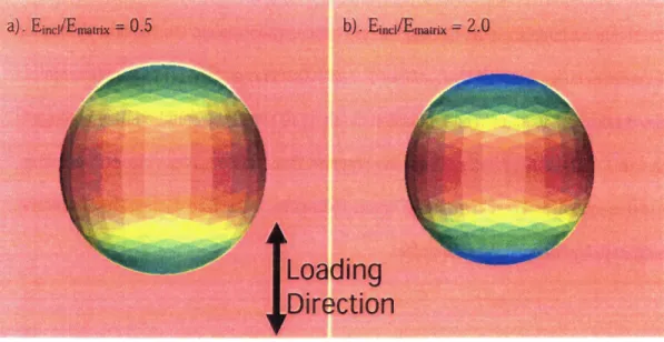
matrix, as shown in Figure 3.1-8a, the highest interface stress on the matrix is located around the equator of the sphere, similar to that of a spherical cavity as shown in Figure 3.1-2. Conversely, when the inclusion has higher Young's modulus than the matrix, as shown in Figure 3.1-8b, the equator area of the matrix has the lowest interface stress. Hence materials with spherical inclusions with lower Young's modulus than the matrix should have the same concern as materials with cavities, namely crack initiation due to stress concentration on the matrix interface. Qualitative comparison of normal traction between the two different inclusions (Figure 3.1-9) shows that while both inclusions have the largest normal traction at the poles, the one with
EiRCIIEmaCrix
> 1 has much higher traction at the poles. This indicates that inclusions having a higher Young's modulus than the matrix are more likely to have crack initiation at the poles through debonding of the matrUinclusion interface than through stress concentration around the equator. This is in fact experimentally observed byLanWbrd J and Kusenberger EN.
[7] in the initiation of fatigue crack in 4340 steel. The inclusions in the 4340 steel they studied likely belonged to the Mn0-Si02-A1203 family. They also reported that while it is not clear if debonding is a prerequisite for crack initiation, crack formation at surface inclusions is always accompanied by debonding at the poles.3.1.5 Stress concentration on cavity and inclusion near a free surface The interaction of second phase structures with a free surface is an important consideration for fatigue and especially in bending and rotation bending applications where maximum stress is found at the surface. The results of our simulation are
for the host material in this test. In previous tests, since the cavity or inclusion is very far
away from the edges, it is possible to use a relatively coarse mesh for the host material
with minimal effect on the result. In the current test on the other hand, a much finer mesh
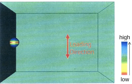
is required for the host because of its interaction with the second phase object. The mesh created for this test is rectangular and measuresl0x7x7. For a spherical object with unit
diameter, a 7 x 7 ~ 1 0 mesh gives a minimum separation of 3 diameters in all other
directions. The figure below shows the rectangular mesh with an inclusion near the
surface.
Figure 3.1-10 Maximum principal stress on host material with an inclusion near a free surface
high
The left side of the rectangle, being closer to the inclusion has a much finer mesh size than the rest of the rectangle. The number of elements on the left wall is 1500 compared to an average of 150 elements on other walls. Even with the relatively high element count
about 0.26, equivalent to a quarter the size of the second phase object. As shall be seen in the following tables, this could possibly account for part of the difference between Julian's simulation result and calculation by
Noda,
MA.and Moriyma
Y. [9] andTable 3.1-7 Stress concentration on 1000-element spherical cavity at distance bid from free surface
I
bld Separation Max. Stress Noda's % Tsuchida's %1
stress conc. result difference result difference0.9 0.056 7705001 3 2.699 3.173 14.94% 3.270 17.46%
Table 3.1-8 Stress concentration on 2000-element spherical cavity at distance bld from free surface
bld Separation Max. Stress Noda's % Tsuchida's %
stress conc. result difference result difference
0.9 0.056 83564756 2.927 3.173 7.76% 3.270 10.49% 0.8 0.1 25 72251 031 2.531 2.759 8.28% 2.760 8.31 % 0.7 0.21 4 66505053 2.329 2.506 7.05% 2.506 7.05% 0.6 0.333 63409871 2.221 2.332 4.76% 2.332 4.76% 0.4 0.750 59374908 2.080 2.145 3.05% 2.1 45 3.05% 0.2 2.000 57646303 2.019 2.092 3.49% 2.092 3.49% - - -(Emat&=
200GPa.
o m a m = 0.25)Table 3.1-9 Stress concentration on 1350-element elliptical cavity at distance bid from free surface
bld Separation Max. Stress Noda's % Tsuchida's %
stress conc. result difference result difference
0.9 0.056 76951 054 2.694 3.104 13.21 %
0.8 0.1 25 731 81 037 2.562 2.829 9.44% 2.829 9.44%
0.6 0.333 72475625 2.537 2.617 3.04% 2.61 5 2.97%
0.4 0.750 72207074 2.528 2.552 0.94% 2.553 0.98%
0.2 2.000 72109260 2.525 2.538 0.53% 2.539 0.57%
Table 3.1-10 Maximum interface stress on 2000-elements spherical inclusion at distance bid from free surface
bld Separation Max interface Applied Stress Noda's % difference stress stress conc. result
0.9 0.056 45236563 3.00E+07 1.508 1.431 5.40% 0.8 0.1 25 42851 656 3.00E+07 1.429 1.503 4.94% 0.5 0.500 41 438377 3.00E+07 1.382 1.431 3.45% 0.4 0.750 41 21 251 3 3.00E+07 1.374 1 -41 8 3.10% 0.3 1.167 41 081 268 3.00E+07 1.370 1.41 2 3.00% 0.1 4.500 40984686 3.00E+07 1.366 1.408 2.95%
Table 3.1-1 1 Maximum normal traction on 2000-elements spherical inclusion at distance bld from free surface
bld Separation Max normal Applied Normalized Noda's % difference traction stress traction result
0.9 0.056 38242572 3.00E+07 1.275 1.210 5.38% 0.8 0.1 25 38292773 3.00E+07 1.277 1.21 6 4.99% 0.5 0.500 383801 42 3.00E+07 1.280 1.21 6 5.23% 0.4 0.750 38401 993 3.00E+07 1.280 1.216 5.29% 0.3 1 . I 6 7 38420457 3.00E+07 1.281 1.21 7 5.26% 0.1 4.500 383991 20 3.00E+07 1.280 1.21 7 5.20%
Figure 3.1-11 Reproduction of a figure in Noda, NA. and Moriyama Y. (2004) showing the test setting of a spherical inclusion in an semi-infinite body under uniaxial load
The distance of the cavity or inclusion from the free surface is given by the ratio bld,
where b is the radius of the sphere (b=0.5) and d is the distance from the center of sphere
to the free surface. "Separation" in the second column presents that same distance in units
of cavity or inclusion diameter. The difference between Julian's simulation result and
discussed above, this larger difference can possibly be attributed to a coarsely meshed wall. Using a high element count mesh for the cavity appears to reduce the difference as
Table 3.1-7 and Table 3.1-8. The gain in accuracy with higher element mesh seems to be more pronounced as the cavity gets closer to the free surface. Therefore one way to improve accuracy in these tests is to increase the element density on the wall but in a way that preserves computational efficiency. Creating a mesh that gradually increases the density of elements towards the center of the wall is a possible solution to this challenge.
It has been mentioned before that Julian tends to underestimate stress concentrations and tractions. However in the case of an A1203 inclusion, Julian appears to consistently overestimate the maximum normal traction by about 5% as compared to Noda's calculation. It is unclear whether Julian actually overestimates in this case because when compared to the analysis in Figure 3.1-7, Julian still reports a slightly underestimated value. By comparing the inclusion results here with the ones in the infinite body case (see Figure 3.1-6 and Figure 3.1-7)' it appears that Noda's calculation does not converge to the infinite body value even with a relatively large wall-to-wall separation of 4.5 between the inclusion and the wall. On the other hand, Julian's result converges nicely to that of the infinite body case at small b/d values (see Table 3.1-5 and Table 3.1-6). In fact, a similar trend is noticed in the spherical cavity test as well (see
Table 3.1-7 and Table 3.1-8). Using Equation 3- 1, the stress concentration on a spherical cavity in an infinite medium with Poisson's ratio of 0.25 is calculated to be 2.022. Julian seems to converge to this infinite body value faster than both Noda's and Tsuchida's calculation.
Graph 3.1-2 shows stress concentration and normalized traction as a function of the wall-to-wall separation between the cavity and the free surface. It is clear from the graph that the maximum normal traction on an inclusion with a E ratio (EjnCI/EmaYd
above 1 behaves very differently from the other curves. Maximum traction seems to be not at all sensitive to its location relative to the wall. In fact, the normal traction fluctuates by only about 0.4% throughout the range of bld values from 0.1 to 0.9. While stress concentration increases as a second phase object approaches the wall, the maximum normal traction on an inclusion with E ratio above 1 actually decreases slightly. This tendency is also noticed in Noda's calculation.
Geometry also affects the shape of the curve in the stress vs. separation graph. According to Graph 3.1-2, an elliptical cavity converges much more rapidly to the infinite body value than a spherical one. In addition, despite generally having a higher stress concentration, an elliptical cavity appears to do better than a spherical cavity, in terms of lesser stress concentration, when it is very close to a wall. However, since we have not considered the minor axis of an ellipsoid in the definition of separation, it is possible that the previous observation becomes invalid as the definition changed. Graph 3.1-2 also shows that if a material has porosity and weaker inclusions (i.e. E ratio less