Bayesian nonparametric approaches for reinforcement learning in partially observable domains

Bayesian Nonparametric Approaches for

Reinforcement Learning in Partially Observable

Domains

by

Finale Doshi-Velez

Submitted to the Department of Electrical Engineering and Computer

Science

in partial fulfillment of the requirements for the degree of

Doctor of Philosophy

at the

MASSACHUSETTS INSTITUTE OF TECHNOLOGY

ARCHNES

Qf TECHNOLOGY

LIBRARIES

June 2012

@

Massachusetts Institute of Technology 2012. All rights reserved.

1

Author ...

Department of Electrical Engineering and Computer Science

April 27, 2012

Certified by...

Nicholas Roy

Associate Professor

Thesis Supervisor

()

Accepted by

-

w

_,,

Leslie Kolodziejski

Bayesian Nonparametric Approaches for Reinforcement

Learning in Partially Observable Domains

by

Finale Doshi-Velez

Submitted to the Department of Electrical Engineering and Computer Science

on April 27, 2012, in partial fulfillment of the

requirements for the degree of Doctor of Philosophy

Abstract

Making intelligent decisions from incomplete information is critical in many applica-tions: for example, medical decisions must often be made based on a few vital signs, without full knowledge of a patient's condition, and speech-based interfaces must in-fer a user's needs from noisy microphone inputs. What makes these tasks hard is that we do not even have a natural representation with which to model the task; we must learn about the task's properties while simultaneously performing the task. Learning a representation for a task also involves a trade-off between modeling the data that we have seen previously and being able to make predictions about new data streams. In this thesis, we explore one approach for learning representations of stochastic systems using Bayesian nonparametric statistics. Bayesian nonparametric methods allow the sophistication of a representation to scale gracefully with the complexity in the data. We show how the representations learned using Bayesian nonparamet-ric methods result in better performance and interesting learned structure in three contexts related to reinforcement learning in partially-observable domains: learning partially observable Markov Decision processes, taking advantage of expert demon-strations, and learning complex hidden structures such as dynamic Bayesian networks. In each of these contexts, Bayesian nonparametric approach provide advantages in prediction quality and often computation time.

Thesis Supervisor: Nicholas Roy Title: Associate Professor

Dedication

Acknowledgments

As an undergraduate in 16.410, Principles of Autonomy and Decision-Making, I was present when Nick gave a guest lecture on particle filters-one of his first lectures as a new professor at MIT. I already thought that Al was cool and probability was awesome, but this? Al and probability? I was hooked. Over the years, I'm very grateful to have had an advisor who not only collaborated on my research but helped me discover what research was, with whom I could both agree and disagree, and who encouraged me to follow my passions for even when they took me abroad to study Bayesian nonparametric statistics at the University of Cambridge. I hope that I can emulate his dedication to both his research and his lab in my future career.

I also thank my committee: Zoubin, Leslie, Tomas, and Josh not only personally

provided insightful suggestions for my research, but by welcoming me into each of their groups, they provided opportunities for me to understand these multifaceted problems in a way that would not have been possible otherwise. I am also grateful to all the wonderful people in those groups-RRG, MLG, LIS, CoCoSci-who joined me in innovative research discussions and collaborations and perhaps even more innovative ways to not take work too seriously.

And last but not least: these years would have been extremely dreary without my wonderful family and friends. I owe much to my walking buddies, pub and coffeehouse

discussion friends, pathshala peoples, artists and martial artists, partners in silliness and stories-the many, many wonderful people who made me look forward to each day. I owe much to my family, especially my parents, who never failed to ring no matter how often I forgot to call, and my brother, who never failed to provide both distractions and Costco runs... and finally, I owe much to my husband Javi, my anchor, who never failed to show me where the silver lining was, when I couldn't find

Contents

1 Introduction 11

1.1 Fram ework . . . . 14

1.2 Contributions of this Research . . . . 23

1.3 Document Roadmap . . . . 25

2 Background 27 2.1 Reinforcement Learning . . . . 27

2.1.1 The Partially Observable Markov Decision Process . . . . 29

2.1.2 Bayesian Reinforcement Learning . . . . 31

2.2 Bayesian Nonparametric Statistics: Models and Inference . . . . 33

2.2.1 Hierarchical Dirichlet Process Hidden Markov Model ... 34

2.2.2 Inference . . . . 37

3 Related Work 40 3.1 Defining State . . . . 40

3.2 States from Features of Histories . . . . 41

3.2.1 States as Windows of History . . . . 42

3.2.2 States as History Subsequences: Finite Automata . . . . 43

3.2.3 Predictive State Representations . . . . 45

3.3 States using Hidden Variables . . . . 46

3.3.1 Representation . . . . 48

4 The Infinite Partially Observable Markov Decision Process

4.1 M odel . . . .. . . . . 4.2 Methods ... ...

4.2.1 Belief Monitoring...

4.2.2 Action Selection . . . . 4.3 Infinite Deterministic Markov Models . .

4.3.1 M odel . . . . 4.3.2 Methods . . . .

4.4 Experiments . . . . 4.4.1 Illustrations . . . . 4.4.2 Results on Standard Problems . . 4.4.3 Other action-selection approaches 4.5 Discussion . . . . 5 Nonparametric Policy 5.1 Model . . . .. .. 5.2 Methods . . . .

.

6.3.3 Application: Weather Modeling . . . . 132

6.3.4 Application: Discovery of Neural Information Flow Networks . 133 6.4 Discussion . . . . 136

7 Conclusions and Future Work 139 7.1 When is this useful? . . . . 140

7.2 Directions for Future Work . . . . 142

7.2.1 Choosing a Sufficient Statistic . . . . 143

7.2.2 Fitting and Preventing Overfitting . . . . 144

7.2.3 Algorithms for Implementation . . . . 146

List of Figures

1-1 General Reinforcement Learning Framework . . . . 1-2 Graphical Model for the MDP . . . .

1-3 Graphical Model for the POMDP . . . .

1-4 Graphical model of the Bayesian RL framework. The model m is con-sidered a hidden variable along with the state s. Usually we assume that the world dynamics are stationary, that is mt = mt+i. . . . . 1-5 Graphical Model for the parameters of the HDP-HMM. . . . .

2-1 2-2 2-3 2-4 4-1 4-2 4-3 4-4 4-5 4-6 4-7 4-8 4-9 4-10 14 15 16 19 23

General Reinforcement Learning Framework . . . . 28

Graphical Model for the POMDP . . . . 29

Graphical Model for the HMM . . . . 35

Graphical Model for the HDP-HMM . . . . 37

Graphical Model for the infinite POMDP. . . . . 58

PDFA graphical model . . . . 67

Asymmetric iDMM Graphical Model . . . . 70

Symmetric iDMM Graphical Model . . . . 72

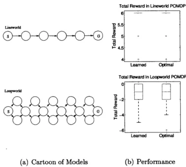
Lineworld and Loopworld Performance . . . . 75

Evolution of Visited State Space Size . . . . 76

Evolution of reward from tiger-3 . . . . 76

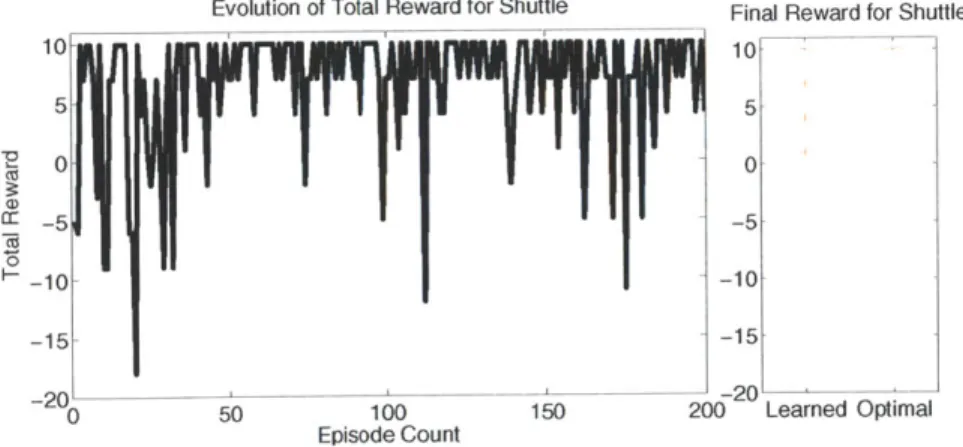
Evolution of Reward in a Single Trial (Shuttle) . . . . 79

Learning Rates over Many Trials (Gridworld) . . . . 80

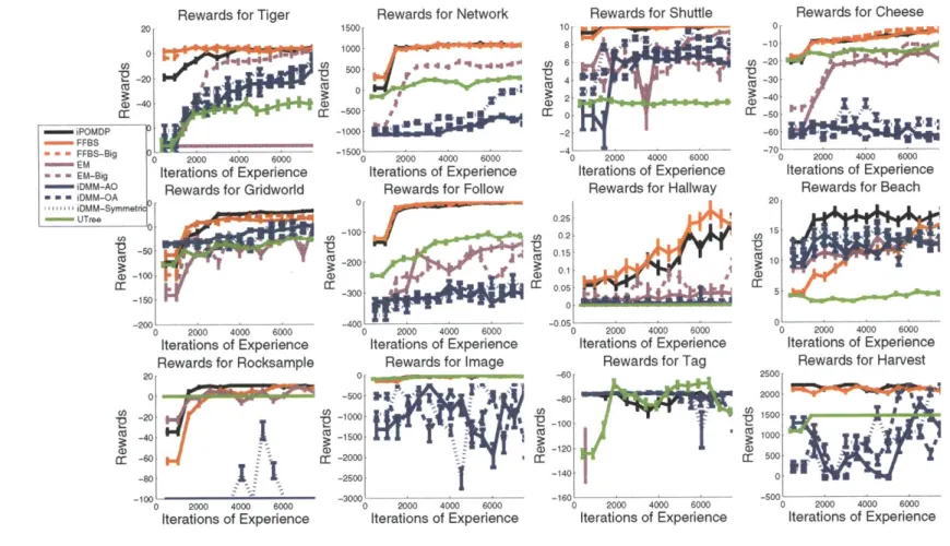
iPOMDP Performance on Benchmark Problems . . . . 81

4-12 4-13 4-14 5-1 5-2 5-3 5-4 5-5 6-1 6-2 6-3 6-4 6-5 6-6 6-7 6-8 6-9 6-10 6-11 83 86 87

iPOMDP State Count on Benchmark Problems . . .

Action Selection Comparison on Tiger . . . .

Action Selection Comparison on Gridworld . . . .

Graphical Model of the Policy Prior Approach . . . .

Graphical Model for the Finite State Controller. . . .

Demonstrations of Policy Priors: Gridworld . . . . . Demonstrations of Policy Priors on Snake . . . .

Policy Priors on Benchmark Problems . . . . Graphical Model of a Dynamic Bayesian Network . . Graphical Model for the iDBN . . . . Growth in hidden nodes for the iDBN, varying aDBN

Toy DBN structure . . . . Finite Model Comparison with Toy DBN . . . . Factors Discovered in the Toy DBN . . . .

Graphical Model of an Infinite Factorial HMM . . .

iDBN Results on Small Weather Dataset . . . . iDBN Structure on Large Weather Dataset . . . .

iDBN Performance on Large Weather Dataset . . . .

iDBN on Zebra-finch Data . . . .

. . . . 93 . . . . 101 . . . . 106 . . . . 107 . . . . 108 115 . 118 120 127 128 129 131 132 134 134 135

List of Tables

4.1 Summary of iPOMDP Benchmarks ... 78

5.1 Policy Priors on Benchmark Problems .... ... 110

6.1 Description of Synthetic Datasets for the iDBN . . . . 130

Chapter 1

Introduction

Imagine exploring a new city for the first time. Busy intersections, quiet plazas, beckoning cafes-there are countless places to see and countless connections between them. Trying to memorize everything from the start is a daunting task, especially when it is unclear what "everything" means: Do we mean every location? Every connecting road? Is it worth remembering where each piece of litter was? Which cor-ners have which street performers? Some kinds of knowledge, such as traffic patterns, cannot be learned immediately: multiple visits to the same intersection are needed to separate pattern from coincidence. When faced with such a challenge, most people will build their model of the city gradually: we may start off by memorizing the few key intersections encountered on our daily commute, and, after some time, we may start to pay attention to finer details such as alternate routes or weekly variations in traffic. Most people will also focus on models that make good predictions: a model that recalls where a particular piece of litter was spotted is less useful for future excursions than a model that learns how late the buses tend to run.

Many sequential decision-making problems exhibit a similar structure in which predictive information is gradually learned from data. Medical decisions must be made based on a limited number of tests and a limited knowledge of the patient's physiology. Still, doctors can often do quite well by starting with a few key principles and refining their knowledge about the patient will react over time. Recommender systems must suggest items that users may wish to buy from a limited purchasing

history. Still, these systems can also do well by starting with notions of items that are generally popular and refining their knowledge about user's preferences over time. Game-playing agents must adjust the difficulty of a player's experience based on a limited number of games. As with the previous examples, these agents can still do well

by trying some basic strategies first and refining their knowledge about the specific

player's strategy over time.

All of the problems above are examples of reinforcement learning in partially

ob-servable domains: reinforcement learning studies how agents can learn to accomplish tasks by collecting experience, and partially observable domains are those in which the agent's entire history of interactions with the environment-whether it is an en-tire clinical record or purchasing history-may be relevant to making future decisions. Reinforcement learning in partially-observable settings is particularly challenging be-cause the history is such a high-dimensional object, and most reinforcement learning approaches rely on different methods to compact histories into lower dimensional knowledge representation. However, the choice of what knowledge representation to use is not always obvious: for example, can all the relevant information in a patient's clinical record be summarized by a set of conditions? How their organs are function-ing at a molecular level? Their genetic sequence? There are often many ways which we can choose to model the data, and each approach will have different gaps and uncertainties.

The work in this thesis addresses this fundamental question in partially observ-able reinforcement learning. Specifically, we demonstrate how Bayesian nonparamet-ric statistics allows agents to incrementally learn about aspects of their environments that have predictive value. The Bayesian aspect of these methods provide ways for the agent to explicitly track its uncertainty and thus focus its knowledge-refinement process toward aspects that are less certain. Bayesian nonparametric methods have the added advantage of increasing the size of the agent's model only as needed to explain the agent's observations. For example, variables corresponding to key condi-tions that affect patient outcomes would be learned before inferring variants of these. Information about a patient's physiology at a molecular level may never be inferred if

simpler structures are sufficient for predicting clinical outcomes. Using Bayesian non-parametric statistics in the learning process results in both reduced computational requirements, as the agents start out with small models and expand them only as need, as well as reduced sample requirements, as agents are able to start performing well early-on by picking up the major trends in the data.

By automatically adjusting the sophistication of the model with the complexity

of the data, Bayesian nonparametric methods provide an approach for learning a representation for a system that is the "right size" for the data. The learned mod-els also have the capacity to incorporate new, unexpected events that may not be present in an initial training set. Of course, not all applications need such flexible or general methods to learn representations. For example, in many robotics and other engineering applications, the representation of the system is known by design, and sensors can be individually calibrated to fit necessary parameters. When designing controllers for dynamical systems, long sequences of data from the relevant operat-ing regimes may be available to perform a more traditional system identification. Bayesian nonparametric methods are best-suited for problems where the choice of the knowledge representation is non-obvious-for example, how to characterize a pa-tient's health or a player's strategy-and it is important to be able to adjust the size of the representation based on sparse data.

The core contributions of this thesis, summarized in section 1.2, are three models for applying Bayesian nonparametric methods to reinforcement learning in partially observable domains. The first, the infinite partially observable Markov decision pro-cess (iPOMDP), posits that the world consists of an infinite number of latent states, and instantiates states as they are needed to explain the agents' observations. The chapter on nonparametric policy priors extends the iPOMDP by considering how to combine expert input with the iPOMDP models learned from the agent's experi-ence. Finally, the infinite dynamic Bayesian network (iDBN) extends the iPOMDP

by considering situations where the latent state of the iPOMDP might be made up

action

observation

reward

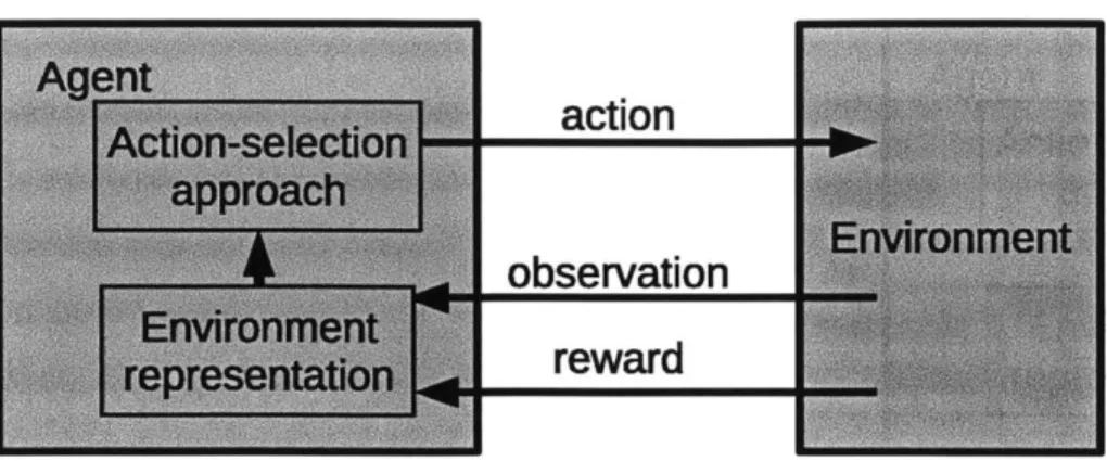
Figure 1-1: General reinforcement learning framework. At each time-step, the agent interacts with the environment with an action and receives an observation and reward.

1.1

Framework

We begin by formalizing the problem of reinforcement learning in partially observable domains. The most general version of the reinforcement learning problem [Sutton and Barto, 1998], summarized in figure 1-1, involves a sequence of exchanges between the agent (left) and the environment (right). At each time step, the agent interacts with the environment through an action a. The environment sends back an observation

o and an immediate reward r. The agent's goal is to maximize the discounted sum

of its expected rewards E[Z± -ytrt], where rt is the reward that the agent receives at time t, and -y

c

rewards.

As a simple example, consider a robot trying to navigate to a goal location. The actions a might correspond to a vector of motor commands, the observations

o might be data from the robot's laser scanner, and the immediate reward r might

indicate whether the robot has reached its destination. Even from this relatively simple scenario, we can see that every element of the agent's interaction history

h = {ao, oo, ro, ..., at, ot, rt} may provide clues as to where the robot is and how it

might try and reach the goal. For example, all corners of a room might produce the same observation o from the laser scanner, but with the entire history of actions and observations h, the agent might be able to disambiguate its position.

Figure 1-2: Graphical Model for the MDP. The shaded nodes s represent the state of the world, which are observed by the agent. The shaded squares a represent the agent's actions, and the shaded nodes r represent the agent's rewards.

Fully Observable Environments A special case of the reinforcement learning framework is one in which the observation o captures all of the information needed to make predictions from the history h. For example, suppose that the robot from the previous scenario had access to an oracle that always provided the robot with its current location. Given its current location, the robot would not require any additional information about its previous locations or previous actions to predict the effect of its next motor command. When the current observation ot captures all of the information needed to predict the future, the environment is described as fully

observable.

One very general way of modeling fully observable environments is with a Markov decision process (MDP, figure 1-2). In this formulation, the environment is modeled as consisting of a set of observed states. At each time step, the agent takes an action a which causes the environment to transition from its current state s to a new state s' based on a transition probability T(s's, a). It also receives a reward R(s, a). The values of the parameters of the transition distributions T and the reward function R are initially unknown. As in the general reinforcement learning framework, the agent's goal is still to maximize the sum of its discounted expected rewards E[L', yt_{rt]. While} there are many ways to model environments, a key property of the MDP formulation is that the dynamics of the system are Markov in the state s-that is, given the

current state st at time t, we do not require any information about the previous states so..st1 to predict the state st+1 at time t

+

Partially Observable Environments Environments in which the dynamics are

not Markov in the current observation ot are called partially observable. A very general way of describing partially observable environments is to assume that the environment is Markov with respect to some now unobserved state s which emits the noisy or partial observation o. For example, even with noisy sensors, the robot's dynamics are still Markov with respect to the robot's position-the only difference is that the robot's position is no longer directly observed. A partially observable Markov

decision process (POMDP, figure 1-3) m is defined by the tuple {S, A, 0, T, Q, R, -Y}

[Sondik, 1971]. S, A, and 0 are sets of states, actions, and observations (all discrete for the purpose of this work). As in the MDP, the transition function T(s'|s, a) gives the probability of transitioning to state s' after performing action a in state s, and the reward function R(s, a) gives the reward for each state-action pair. The observation function Q(ols, a) gives the probability of seeing observation o after taking action a in state s.

St-1

Figure 1-3: Graphical Model for the POMDP. The white nodes s represent the now

hidden state of the world, and the shaded squares a represent the agent's actions.

Action Selection The rule that governs how the agent selects its actions is called a policy -x. When the environment is fully-observable, the current state st encodes everything about the past needed to predict the future; thus, we know that the optimal policy lies in the set of functions ir(s, a) = p(als), which gives the probability

of performing action a in state s. When the environment is partially-observable, all elements of the history ht = {a1, oi, r1, ... , at, ot, rt} might be required to make

predictions about the future. Thus, the optimal policy now lies in the set of functions

r(h, a) = p(alh), which gives the probability of performing action a in state s.

Action-Selection with a Known Model: Planning Before describing how an agent

might select its actions in the reinforcement learning setting, we consider a simpler setting in which the parameters of the POMDP model m = {S, A, 0, T, Q, R, -y} are

given (known as planning). Let the belief bt(s) be the conditional distribution p(st

I

over the current state st given the history ht. If the parameters of the transition and observation functions T and Q are known, it is possible to compute the current belief bt(s) given the previous belief b_1 (s), the current action at, and the current

observation ot:

be(s) = Q(otls, at) E T(sIs', at)bt.1(s'(1.1)

S'ES Pr(otlbt_1, at)

where Pr(olb, a) = Ewes Q(ols', a) ZSEs T(s'ls, a)b(s). Unlike the most recent ob-servation ot, the belief bt(s) captures all the information in the history ht needed to make predictions about the agent's future [Sondik, 1971]. In this sense, we can think of a partially observable environment as a fully observable environment in this high-dimensional, continuous space of beliefs. It follows that the optimal policy for the POMDP must then lie in the space of functions ir(b(s), a) = p(alb(s)), and a

number of algorithms have been developed for finding near-optimal polices for this representation [Bellman, 1957, Littman et al., 1995, Pineau et al., 2003, Spaan and

Vlassis, 2005, Smith and Simmons, 2004, Shani et al., 2007, Kurniawati et al., 2008].

Action-Selection with an Unknown Model: Learning Action-selection is much more

challenging in the more general setting in which the parameters of the model m are not known (and thus update rules like equation 1.1 cannot be used to summarize

the history). Whether the environment is fully observable or partially observable, reinforcement learning-as opposed to planning-involves learning from data, and histories are inherently noisy. Thus, many repetitions of similar situations may be needed to characterize patterns. Second, it is difficult to assign credit for a reward: a high reward rt at time t may be the result of the action at or some action farther back in the past. Finally, without knowing the model m, the agent must balance time spent learning the dynamics (exploration) and maximizing reward (exploitation).

These factors are particularly challenging in the partially observable setting where the optimal policy 7r(alht) is a function of the entire history ht. Because the history

ht contains many more parameters than a single state st, the policy ir(alht) will

require many more samples to learn. Similarly, without more knowledge about the environment, we are forced to start learning a very general reward function R(rjh) rather than having a simpler functional form R(rls). Finally, exploration is more difficult when we have to consider visiting histories h rather than states s. At the same time, these factors also make partially-observable reinforcement learning more general than settings in which the domain is fully-observed or fully-specified: we can operate directly in the space of histories and never think about hidden states or beliefs over hidden states.

Approaches to tackling the partially-observable reinforcement learning problem-that is, learning policies based on histories of experience-vary widely. On one end of the spectrum are methods that never directly model the hidden state and instead choose new actions from the history of past actions and observations. Most of these approaches try to group together histories that require similar actions-for example,

U-Tree [McCallum, 1993] builds a suffix tree on the history, AIXI [Hutter, 2004]

extracts features from the history, and predictive state representations [Singh and James, 2004] learn short-term predictions for a set of test histories. Under relatively mild conditions on the underlying POMDP, history-based approaches can learn near-optimal policies in polynomial time [Even-Dar et al., 2005]. However, even if the sample complexity is polynomial, these algorithms typically require large amounts of experience to convert histories into useful policies. For example, even newer AIXI

implementations, such as that of Veness et al. [2009], require on the order of 104

interactions to learn a very simple POMDP (tiger [Littman et al., 1995]), whereas a model-based Bayesian method such as BA-POMDP [Ross et al., 2008a] requires on the order of 102 interactions for the same problem.

On the other end of the spectrum are Bayesian methods which explicitly consider beliefs not only over potential hidden states but also over possible models [Poupart and Vlassis, 2008, Jaulmes et al., 2005, Ross et al., 2008a, Strens, 2000, Dearden et al.,

1999, Ross et al., 2008b, Doshi et al., 2008, Duff, 2002]. These approaches note that

reinforcement learning problem can be thought of as a planning problem in which both the agent's current state st and the world model m are hidden. Bayesian methods start out with a prior distribution over models p(m) and then track the joint distribution

bt(s, m) = pt(s, m) over the current state and the world model m. As with a standard

POMDP, the joint belief bt(s, m) is a sufficient statistic for the history: it encodes everything about the past needed to make future predictions. Thus, the optimal reinforcement learning policy lies in the set of functions r(b(s, m), a) which requires solving a larger "model-uncertainty" POMDP (see graphical model in figure 1-4).

(a) Graphical model for the Bayesian (b) Expansion of the graphical model showing a single

RL framework, showing both the model time-slice in the model-uncertainty POMDP; gray and

and the current state as hidden nodes black arrows are equivalent (colored only for clarity).

Figure 1-4: Graphical model of the Bayesian RL framework. The model m is con-sidered a hidden variable along with the state s. Usually we assume that the world dynamics are stationary, that is mt = men.

The Bayesian reinforcement learning setting also offers an elegant formulation for incorporating expert knowledge: the starting belief bo(s, m) can encode one's prior be-liefs over what models m are likely. In general, Bayesian methods need fewer samples of experience (that is, fewer histories) to learn good policies. However, actually doing computations on the belief b(s, m)-such as applying equation 1.1-can be challeng-ing because the model m itself consists of the many parameters contained in TQ,and

R. Different Bayesian reinforcement learning methods present different

approxima-tions of standard POMDP planning techniques for this more complex space where we maintain distributions over both possible current states and possible models. The cost of the associated computations-having to reason about all the unknown parameters in have typically restricted these methods to small problems. Unlike model-free or history-based approaches, another difficulty with these approaches is that the structure of the hidden part of the underlying model, for example, the number of states or sets of factors, must now be specified.

Despite the variety of approaches and continued interest in partially observable reinforcement learning [Hutter et al., 2009], several factors have limited their success. First, much recent work-especially the Bayesian literature-has focused on inferring the dynamics of the true underlying system, rather than predicting how the system will respond to various inputs. While sometimes a reasonable goal, explicitly trying to infer the true system can make the learning problem unnecessarily challenging, especially when accurate predictions are all that are required for decision-making. In these cases, reasoning about extra model parameters is wasted computational effort. Current inference techniques also tend to converge to sub-optimal solutions. Finally, expert information is often incorporated in ways that impose rigid constraints on the model, rather than more targeted use of the agent's own experience.

Bayesian Nonparametric Model Learning This thesis examines how Bayesian nonparametric techniques can address many of the challenges we outlined for partially-observable reinforcement learning. A Bayesian nonparametric model defines a distri-bution over an infinite-dimensional parameter space [Orbanz and Teh, 2010]. For

example, in this thesis, we consider an extension of the POMDP in which the model

m has an infinite number of hidden states s, and thus an infinite number of

pa-rameters are needed to describe the transitions T(s'Is, a), observations Q(ols, a), and rewards R(s, a). Like more traditional Bayesian approaches to reinforcement learn-ing, we define an initial prior p(m) over models m and update this prior belief as the agent gathers experience; as before, our use of Bayesian nonparametric methods for reinforcement learning involves casting the partially-observable reinforcement learn-ing problem as solvlearn-ing the model-uncertainty POMDP in which the belief bt(s, m) is the proxy for the state. In doing so, we inherit many of the benefits of Bayesian approaches to reinforcement learning, including a clear optimization criterion and relatively low sample complexities for learning reasonable policies.

However, unlike more traditional Bayesian reinforcement learning approaches, which try to recover a model of the environment [Ross et al., 2008a, Jaulmes et al.,

2005, Poupart and Vlassis, 2008, Dearden et al., 1999, Duff, 2002, MacKay, 1997], our

emphasis is simply to be able to make good predictions. Drawing on concepts from

Stolcke and Omohundro [1993], Shalizi and Shalizi [2004], and Drescher [1991], using

Bayesian nonparametric methods allow us to think of hidden states not as physical aspects of the environment, but as "way-points" that are needed to make the under-lying system Markovian. Using an approach that assumes that the world contains an infinite number of underlying states ensures that we will always have enough way-points to explain our observations. However, the prior p(m) ensures that states are instantiated only if the current set of instantiated states do not explain the data well. Models instantiated in this incremental fashion often have fewer instantiated parame-ters than the "true" model, making them easier to learn and solve. Finally, the same Bayesian nonparametric methods used to keep distributions over models-that is, how the world works-can be used to keep distributions over well-performing policies

r(h, a)-that is, how the agents should behave.

In the context of modeling dynamical systems, one of the core Bayesian nonpara-metric models used in this work is the infinite Hidden Markov Model (HDP-HMM)

[Beal et al., 2001, Teh et al., 2006],1 A hidden Markov Model (HMM) is essentially a POMDP without the decision-making component: it does not have actions or re-wards, but it still posits that the environment consists of a set of hidden states s that transition according to some transition function T(s'|s) and emit observations according to some observation function Q(ols). The HDP-HMM places a distribution p(m) over HMM tuples m =

{S,

1. Draw the mean transition distribution

T

2. Draw observation distributions

Q(-Is)

3. Draw transition distributions T(.Is) - DP(a, T) for each state s.

where Stick() represents a stick-breaking procedure based on the Dirichlet process (DP) [Ferguson, 1973, Teh, 2010], A is the DP concentration parameter, and H is a prior over observation distributions. For example, if the observations are discrete, then H could be a Dirichlet distribution from which multinomials over the observa-tions are drawn.

This sampling procedure produces HMM models m that have an infinite number

of states but whose histories ht = {so, o0, ... , st, Ot} typically visit only log(t) states.

The first step, drawing

T,

Tk to each state k such that the sum of the popularities is one: E'

T

Dirichlet process provides a bias toward having a few popular states (states k such that Tk > 1 and and very many unpopular states (states k such that Tk < )

By using these popularities

T

'The iHMM models in Beal et al. [2001] and Teh et al. [2006] are formally equivalent [Gael and Ghahramani, 2010].

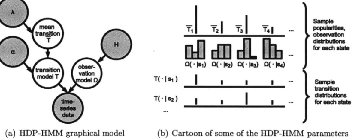
for a robot, a new set of preferences for a recommender system, a new type of condition for a patient. Figure 1-5 shows the graphical model of the parameters of the

HDP-HMM. _

11

Ti

_f

...

I

(a) HDP-HMM graphical model (b) Cartoon of some of the HDP-HMM parameters

Figure 1-5: Graphical Model for the parameters of the HDP-HMM.

Our work follows a variety of works in which Bayesian nonparametric models have been used to estimate models of dynamical systems. Many of these [Fox et al.,

2010a, 2008, Stepleton et al., 2009, Johnson and Willsky, 2010] are variants of the

HDP-HMM. Other approaches [Stolcke and Omohundro, 1993, Shalizi and Shalizi,

2004], while they not explicitly define Bayesian nonparametric models, have a similar flavor to Bayesian nonparametric models in that they automatically infer the size and structure of the underlying model. However, only in rare cases have these models been used for controlling as well as learning systems, and previous work that has used Bayesian nonparametric methods for reinforcement learning [Engel et al., 2005, Deisenroth et al., 2009] has focused largely on continuous domains.

1.2

Contributions of this Research

The core contribution of this thesis is showing how Bayesian nonparametric methods provide a different way about thinking about state in reinforcement learning; indeed, Bayesian nonparametric methods are a natural fit for sequential decision-making prob-lems in which parts of the world can only be learned about once experienced. More

specifically, we present three Bayesian nonparametric models and empirically demon-strate their value for reinforcement learning in partially observable domains.

Infinite POMDPs. Our first model is the infinite POMDP (chapter 4). Building on the HDP-HMM [Beal et al., 2001, Teh et al., 2006], the infinite POMDP posits

that the (now controlled) world consists of an infinite number of states. As with the HDP-HMM, the states in an infinite POMDP are no longer identifiable; they do not necessarily correspond to the "true" underlying states of the world. Instead, the concept of a state is a way-point that is useful for making future predictions, something that makes the underlying system more Markovian. We show that learning the state gradually allows us to learn enough to capture the key dynamics of the system, resulting in learning that both requires fewer samples and is computationally more efficient than learning the full "true" model. The next two contributions extend this basic work in two orthogonal directions.

Nonparametric Policy Priors. In chapter 4, the infinite POMDP model is learned only from the agent's own experience. An agent's actions do not provide information about the world; they are simply its policy. However, in some settings, it may be possible to get demonstration trajectories from an expert. As with the agent's data, the expert histories can be used to learn more about the world dynamics T, Q, and

R. However, they provide an additional source of information: the expert's actions

are presumably near-optimal. Combining this information with self-exploration is tricky because self-exploration provides direct information about the model, while demonstrations provide direct information about the optimal policy. In chapter 5, we provide a principled way to combine agent experience with expert demonstrations through a model prior that jointly prefers models with fewer states and simpler poli-cies. As expected, combining expert demonstrations with self-exploration results in faster learning for performance.

Infinite Dynamic Bayesian Networks. The infinite POMDP describes the

make sense to think of the hidden state as consisting of several hidden factors: a robot may have unknown position and velocity; each of a patient's organ systems may be in a different state of health. In chapter 6, we introduce a very flexible prior over factored hidden state spaces, the infinite Dynamic Bayesian Network (iDBN). This prior allows for an infinite number of hidden factors, each of which can take on an arbitrary number of discrete values and have arbitrary inter-node connections. We do not demonstrate the iDBN on a sequential decision-making task, but we do show that it finds interesting, predictive structures compared to other DBN-learning approaches.

1.3

Document Roadmap

This document contains three major sections. First, chapter 2 expands the formalisms introduced in section 1.1, providing the key technical background to read this thesis as a stand-alone text. Chapter 2 also provides pointers to additional papers and tutorials in these fields.

Second, chapters 3 and 7 places the work in the context of other work in rein-forcement learning and different types of application domains. Chapter 3 describes related work in partially observable reinforcement learning, focusing on the different notions of state used by different methods. We also describe how the notion of state in Bayesian nonparametric methods relates to these other approaches. Chapter 7 sum-marizes the empirical results of this thesis, relating these results to what we might expect from a Bayesian nonparametric framework.

Finally, chapters 4, 5, and 6 contain our technical contributions. Many of the contributions in these chapters are already summarized in earlier work [Doshi-Velez, 2009, Doshi-Velez et al., 2010, 2011]. However, chapter 4 in particular has been greatly expanded: not only have we included a thorough evaluation of the iPOMDP in many more domains, we also show the effect of several action-selection strategies on the agent's overall performance. We also provide comparisons be-tween the iPOMDP and a new history-based Bayesian nonparametric model based

on probabilistic-deterministic infinite automata.

More generally, this thesis presents the technical chapters in a more unified man-ner, with some expanded results, the key additions to this work over the more con-densed conference articles are expanded sections on inference and discussion. A spe-cial effort has been made to include details and tricks needed to make these models "behave" and to also include where these techniques fail. To this end, each of the three main chapters of the thesis are presented in an identical four-part structure: models, methods, results, and discussion. The models section of each chapter de-scribes the generative process that defines the prior for each model, making explicit key assumptions and discussing how these assumptions manifest themselves in prac-tice. The methods section of each chapter describes the inference techniques needed to

derive a posterior over models given data, with a focus on including inference details often glossed over in shorter documents. The results section contains an empirical validation of the approach on various benchmark problems, followed by a discussion on when these techniques work best.

Chapter 2

Background

The work in this thesis combines two areas of machine learning: Bayesian nonpara-metric statistics and partially-observable reinforcement learning. In this chapter, we provide a brief overview of these areas, as well as pointers to further information. Models for specific applications, such as finite state machines or dynamic Bayesian networks, are described in the chapters in which they appear.

2.1

Reinforcement Learning

The field of reinforcement learning (RL) is characterized by sequential decision-making problems in which the agent's goal is to maximize long-term reward in unknown environments. Specifically, reinforcement learning involves a sequence of exchanges between the agent and the environment. At each time step, the agent interacts with the environment through an action a. The environment sends back an observation o and an immediate reward r (figure 2-1). The agent's goal is to maxi-mize the discounted sum of its expected rewards E[EZ -ytrt], where rt is the reward that the agent receives at time t, and y E [0, 1) trades off between the importance of current rewards and future rewards (see Sutton and Barto [1998] for a much more complete introduction).

Three elements differentiate reinforcement learning from related problems in con-trol and optimization. First, we assume that the agent must interact with the

envi-action

observation

reward

Figure 2-1: General reinforcement learning framework. At each time-step, the agent interacts with the environment with an action and receives an observation and reward. The observation and reward are used to update the agent's representation of the environment and then to select the next action.

ronment over time: all reinforcement learning problems have an element of sequential decision-making. Second, the agent learns through only an immediate reward signal: through trial, error, and inference, the agent must distinguish which actions were responsible for its rewards. Finally, the learning process is sample-based: the agent does not start out with a complete model of the environment and then makes sequen-tial decisions; any and all aspects of the environment must be learned through the agent's experience of experience.

As with most reinforcement learning problems, the partially observable reinforce-ment learning problem can be divided into two parts [Hutter et al., 2009]: choosing a representation for the environment and deciding how to act given that representation. We emphasize that the representation is internal to the agent: it is how the agent chooses to encode its knowledge about its environment, not the environment itself. In general, the representation will consist of two parts: a part that summarizes the current history ht and a part that encodes general (usually static) information about the environment. For example, the simple robot from chapter 1 might be simultane-ously keeping a distribution over its current location-which summarizes its history ht-while building a (static) map of its environment. Both of these parts are needed to choose actions.

2.1.1

The Partially Observable Markov Decision Process

In this section, we provide a description of one popular representation, the partially-observable Markov decision process [Sondik, 1971, Kaelbling et al., 1995]. (Other representations are summarized in chapter 3.) A POMDP m is specified by the tuple

{S,A,O,TQ,R,y},

At each time-step, the transition function T(s'|s, a) gives the probability of transi-tioning to state s' after taking action a in state s (figure 2-2). The agent then receives an immediate reward R(s, a) for taking action a in state s. What makes the domain partially-observable is that the agent does not also receive the state s. Instead, it only receives an observation ot which is emitted from the state st with probability Q(ols, a). For example, the observation ot might be a laser scan from the robot's true position st. Unlike the current state st, the current observation ot is not sufficient for summarizing the agent's position, and the best action to take at time t may require

information from the agent's entire history ht = {a1, oi, r1, ..., at, ot, rt} of previous

actions, observations, and rewards.

Figure 2-2: Graphical Model for the POMDP. The white nodes s represent the hidden state of the world, and the blue squares a represent the agent's actions. The blue nodes o and r represent the observations and rewards.

As we noted in section 1.1, while POMDPs are not Markovian in the current observation ot, the current distribution over possible states, called the belief bt(s), does capture all the information in the history ht needed to predict future events. In discrete state spaces, the belief at time t

+

Vt j () =Q o I, a E T(s Is', a) bt (s')(21

bg"1(s) =

~

Po

a),(21

s'ES

where Pr(ol b, a) =

E,,Es

Q(ols',

Because the POMDP dynamics are Markovian in the space of beliefs bt(s), the optimal policy is contained in the set of functions ir(b(s), a) = p(alb(s)) that give the probability of taking action a in belief b. Let VW (b) be the expected long-term reward associated with starting in belief b and then following a policy 7r. The value of V(b) can be computed using the Bellman equations [Bellman, 1957]:

V"(b) =

Z 7r(b, a)(R(b, a)

y E

a OEO

where we use the notational shorthand r(b, a) = ,7r(s, a)b(s), and R(b, a) =

E,

Solving equation 2.2 gives us the value V" of a specific policy r. For a belief b, optimal policy r*, that is, the policy that achieves the highest long-term rewards, can be found by first solving for the value of the optimal policy V'* (b):

V*(b) = maxQ*(b, a), (2.3)

aEA

Q*(b,

a)

=

R(b, a) + -y

Pr(ob, a)V*(ba"O),

(2.4)

oEO

optimally. The optimal policy is then

r*(b) = arg max Q*(b, a). (2.5)

The exact solution to equations 2.4 and 2.5 is only tractable for tiny problems, but many approximation methods [Pineau et al., 2003, Spaan and Vlassis, 2005, Smith and Simmons, 2004, Shani et al., 2007, Kurniawati et al., 2008] have been developed to solve POMDPs offline. For even larger problems, forward search techniques can be used to find solutions online [Ross et al., 2008c].

As with all planning and reinforcement learning techniques, an agent using a POMDP as its knowledge representation alternates between two phases when inter-acting with its environment. Upon receiving an observation, the agent updates its belief over states bt(s) given the previous belief bt_1, the current action at, and the current observation ot using equation 2.1. This representation update is known as be-lief monitoring or estimation. Second, in the action selection phase, the agent selects its next action given its current belief be(s) and equations 2.4 and 2.5. While differ-ent approximations may be used for each of these phases, the phases themselves-incorporating new information (belief monitoring) and then choosing a new action (action selection)-are common to all approaches for acting in POMDPs.

2.1.2

Bayesian Reinforcement Learning

In the reinforcement learning setting, of course, the agent does not have access to the parameters of the model T, Q, and R; the model m must be learned from the agent's interactions with the world. In the Bayesian reinforcement learning setting, the agent starts out with a prior distribution p(m) over possible models. Given a dataset D of histories h, the agent can compute a posterior over possible models p(mfD) oc P(Djm)P(m). The model prior p(m) can encode both vague notions, such as "favor simpler models," as well as strong structural assumptions, such as topological constraints among states.

equivalent-to the initial belief bo(s) placed over agent states in section 2.1.1. As discussed in Duff [2002], if we think of the prior as an initial belief over models, we can cast the problem of acting in an environment without a known model as a "model-uncertainty" POMDP in which both the model m and the state of the world

s are hidden from the agent. We can factor the joint belief b(s, m) as

b(s, m) = b(slm)b(m). (2.6)

Conditioned on data D from the agent's histories h, we get

b(s,mjD) = b(slm,D)b(mID). (2.7)

The first term b(slm, D) can be computed using the belief update in equation 2.1. The second term b(mID) is simply the posterior over models p(m|D). Describing the reinforcement learning problem as just a very large POMDP implies that now we can use equations 2.4 and 2.5 to determine an optimal policy to maximize expected discounted rewards, even if the dynamics are not initially known.

Of course, having a decision-theoretic formulation of the Bayes-optimal policy

does not imply that solving for the policy is computationally tractable. Methods for approximating the optimal policy include sampling a single model m from the posterior belief bt (m|D) and following that model's optimal policy p* (b, aIm) for a fixed period of time [Strens, 2000]; sampling multiple models and choosing actions based on a vote or stochastic forward search [Jaulmes et al., 2005, Doshi et al.,

2008, Doshi-Velez, 2009, Ross et al., 2008a]; and trying to approximate the value

function for the full model-uncertainty POMDP analytically [Poupart and Vlassis,

2008]. Other approaches [Wang et al., 2005, Kolter and Ng, 2009, Asmuth et al., 2009] try to balance the off-line computation of a good policy (the computational

2.2

Bayesian Nonparametric Statistics: Models and

Inference

In statistics, a model is a probability distribution p(xlj), where x is some set of data and 9 is some set of parameters. The core concept of a Bayesian nonparametric model involves the combination of two ideas: Bayesian models and nonparametric models (see Orbanz and Teh [20101 for a much more detailed overview). A Bayesian model is one in which the parameters of the distribution 9 are themselves random variables with some prior distribution p(9). We can think of the prior p(O) as the distribution over the values that we believe that the parameters 9 might take before we have seen any data. The posterior distribution p(9|x) captures our uncertainty over the values that the parameters 9 might take after seeing the data x. Nonparametric models are models for which the parameter space 9 is infinite-dimensional. Thus, a Bayesian nonparametric model is some probability distribution p(xl9) in which 0 is an infinite-dimensional random variable.

There are two ways in which the prior p(O) can be specified. Explicit

represen-tations provide a procedure for first sampling the parameters 0 - p(9) and then the

data x - p(xl9). Having explicit procedures for sampling the parameters and the data

ensures that our prior p(O) is in fact a probability distribution and that a finite sam-ple of data can be explained by a finite number of parameters. In contrast, implicit representations describe a procedure for generating the data without explicitly sam-pling the parameters 9 first (beneficial because the number of parameters is infinite!). When the prior p(O) is never used explicitly, statistical results such as de Finetti's theorem or the Kolmogorov Extension theorem must be applied to ensure that the procedure used to generate the data implies a valid distribution p(9). The properties of models are often clearer when the generative process is explicit; inference is often simpler with implicit representations.

Inference, or computing the posterior p(O|x), requires special care when the pa-rameter vector 0 is infinite-dimensional. The Bayes equation p(Olx) oc p(xI9)p(9) may not technically exist because the family of all possible posteriors do not dominate,

or overwhelm, the prior. However, conjugacy can allow the posterior p(9|x) to be computed given the data x and the prior p(O). A properly defined Bayesian nonpara-metric model has the following properties: First, even though the parameter vector

O is infinite-dimensional, we require that a finite sample of data x = {x1 ) -.., X, } can

be modeled with only a finite number of those dimensions. Second, asymptotic con-sistency requires that the effect of the prior p(O) disappears with sufficient data (or, alternatively, given infinite data, the parameters will converge to their true values with probability one). A third desirable, but not required, property for these models is exchangeability, which states that the ordering of the data points does not matter when evaluating their probability.

In the remainder of this section, we describe one particular Bayesian nonparamet-ric model, the hierarchical Dinonparamet-richlet process hidden Markov model (HDP-HMM), that we use extensively in this work. We also provide and overview of several inference techniques that can be used to sample from the posterior over parameters p(0|x), which will be necessary for representing the belief over models b(m).

2.2.1

Hierarchical Dirichlet Process Hidden Markov Model

A standard hidden Markov Model (HMM) [Rabiner, 1989] is a model for time-series

data which consists of the tuple m = {S, 0, T, Q}. The set S is the set of world-states,

and the set 0 is the set of observations accessible to the agent. At each time-step, the current state st emits an observation ot drawn from a distribution Q(-|s) and transitions to a new state st+1 drawn from a distribution T(-Is) (figure 2-3). One can think of the HMM as the part of the POMDP that describes how world-states change without the components relevant for decision-making (actions and rewards).

Bayesian approaches to learning HMMs involve putting priors over the transition distributions T and the observation distributions Q. When the set of states S and the set of observations 0 are discrete and finite, the multinomial distributions are the most general choice for the transition distribution T(-Is) and the observation distributions f2(-ls). As conjugate distributions to the multinomial, Dirichlet distributions are thus a natural choice of priors p(T(-Is)) and p(Q(-|s)).

Figure 2-3: Graphical Model for the HMM. The blue observation nodes o are the variables that are observed at each time-step {...t - 1, t, t

+

represent the hidden state of world.

The infinite Hidden Markov Model, also known as the hierarchical Dirichlet pro-cess Hidden Markov Model (HDP-HMM) [Beal et al., 2001, Teh et al., 2006] places a prior over worlds whose state spaces S are discrete but countably infinite. In the HDP-HMM, the transition distributions T are still multinomials, but over an infinite number of states s. Thus, the natural conjugate prior for a particular transition dis-tribution p(T(-Is)) is now a Dirichlet process [Ferguson, 1973, Teh, 2010] rather than a Dirichlet distribution. Using a hierarchical Dirichlet process as a prior for the set of transition distributions T ensures that all the distributions T(.s) are over the same state space S. It also encodes the prior belief that there are a few popular states to which all states transition.

A formal overview of the HDP-HMM first requires a summary of the Dirichlet

process. Recall that a multinomial distribution d with K elements can be encoded

by a set of pairs {(Xk, 0)} for k = 1...K, where 3k is the probability of sampling the element Xk. (Note that

Z

#K

the three colors red, yellow, and blue could be written as

{

( blue , .6 )

}.

#k)}

Xk.

The following explicit representation provides the generative procedure to draw a multinomial distribution d = {(Xk, kI)} from a Dirichlet process prior DP(A, H):

1. Draw the samples Xk ~ H for k = 1...oo. The samples Xk define where the