Publisher’s version / Version de l'éditeur:
Vous avez des questions? Nous pouvons vous aider. Pour communiquer directement avec un auteur, consultez la
première page de la revue dans laquelle son article a été publié afin de trouver ses coordonnées. Si vous n’arrivez pas à les repérer, communiquez avec nous à [email protected].
Questions? Contact the NRC Publications Archive team at
[email protected]. If you wish to email the authors directly, please see the first page of the publication for their contact information.
https://publications-cnrc.canada.ca/fra/droits
L’accès à ce site Web et l’utilisation de son contenu sont assujettis aux conditions présentées dans le site LISEZ CES CONDITIONS ATTENTIVEMENT AVANT D’UTILISER CE SITE WEB.
Seventh SIAM International Conference on Data Mining (SDM 2007)
[Proceedings], 2007
READ THESE TERMS AND CONDITIONS CAREFULLY BEFORE USING THIS WEBSITE. https://nrc-publications.canada.ca/eng/copyright
NRC Publications Archive Record / Notice des Archives des publications du CNRC :
https://nrc-publications.canada.ca/eng/view/object/?id=94871dbd-2488-45c8-8818-2079f15ad927 https://publications-cnrc.canada.ca/fra/voir/objet/?id=94871dbd-2488-45c8-8818-2079f15ad927
NRC Publications Archive
Archives des publications du CNRC
This publication could be one of several versions: author’s original, accepted manuscript or the publisher’s version. / La version de cette publication peut être l’une des suivantes : la version prépublication de l’auteur, la version acceptée du manuscrit ou la version de l’éditeur.
Access and use of this website and the material on it are subject to the Terms and Conditions set forth at
Fast & confident probabilistic categorisation
Fast & Confident Probabilistic
Categorisation*
Goutte, C.
2007
* published at the Text Mining Workshop. 2007. NRC 49286.
Copyright 2007 by
National Research Council of Canada
Permission is granted to quote short excerpts and to reproduce figures and tables from this report, provided that the source of such material is fully acknowledged.
Fast & Confident Probabilistic Categorisation
Cyril GoutteInteractive Language Technology
National Reasearch Council Canada, Institute for Information Technology 101 rue St-Jean-Bosco, Gatineau, QC K1A 0R6, Canada
February 15, 2007
Abstract
We describe NRC’s submission to the Anomaly Detection/Text Mining competition organised at the Text Mining Workshop 2007. This submis-sion relies on a straightforward implementation of the probabilistic categoriser described in [4]. This categoriser is adapted to handle multiple labelling and a piecewise-linear confidence esti-mation layer is added to provide an estimate of the labelling confidence. This technique achieves a score of 1.689 on the test data.
1
Overview
This paper describes NRC’s submission to the Anomaly Detection/Text Mining competition organised at the Text Mining Workshop 2007 (http://www.cs.utk.edu/tmw07/). This submis-sion relies on an implementation of the proba-bilistic categoriser described in [4], without us-ing any hierarchical structure. As a consequence, training is extremely fast and requires a sin-gle pass over the data to compute the summary statistics used to estimate the parameters of the model. Prediction requires the use of an itera-tive maximum likelihood technique (Expectation Maximisation, or EM, [2]) to compute the pos-terior probability that each document belongs to each category.
In the following section, we describe the prob-abilistic model, the training phase and the al-gorithm used to provide predictions. We also address the problem of providing multiple la-bels per documents, as opposed to assigning each
document to single category. We also discuss the issue of providing a confidence measure for the predictions and describe the additional layer we used to do that.
Section 3 describes the experimental results obtained on the competition data. We provide a brief overview of the data and we present results obtained both on the training data (estimating the generalisation error) and on the test data (the actual prediction error).
2
The probabilistic model
Let us first introduce some formal notation. In a text categorisation problem, such as proposed in the Anomaly Detection/Text Mining competi-tion, we are provided with a set of M documents dand associated labels ℓ ∈ {1, . . . C} where C is the number of categories. These form the train-ing set D = {(di, ℓi)}i=1...M. Note that, for now,
we will assume that there is only one label per document. We will address the multi-label sit-uation later in section 2.3. The text categorisa-tion task is the following: given a new document
e
d6∈ D, find the most appropriate label ℓ. Theree are mainly two flavours of inference for solving this problem [14]. Inductive inference will esti-mate a model fbusing the training data D, then assign deto label fb(d). Transductive inferencee will estimate the label ℓe directly without esti-mating a general model.
We will see that our probabilistic model shares similarities with both. We estimate some model parameters, as described in section 2.1, but we do not use the model directly to provide the la-1
bel of new documents. Rather, prediction is done by estimating the labelling probabilities by max-imising the likelihood on the new document us-ing an EM-type algorithm, as described in sec-tion 2.2.
Let us now assume that each document d is composed of a number of words w from a vocab-ulary V. We use the bag-of-word assumption. This means that the actual order of words is dis-carded and we only use the frequency n(w, d) of each word w in each document d. The cat-egoriser presented in [4] is a model of the
co-occurrences (w, d). The probability of a
co-occurrence, P (w, d) is a mixture of C multino-mial components, assuming one component per category: P(w, d) = C X c=1 P(c)P (d|c)P (w|c) (1) = P (d) C X c=1 P(c|d)P (w|c)
This is in fact the model used in
Probabilis-tic Latent SemanProbabilis-tic Analysis [8], but used in a
supervised learning setting. The key modelling aspect is that documents and words are condi-tionally independent, which means that within each component, all documents use the same vo-cabulary in the same way. Parameters P (w|c) are the profiles of each category, and parameters P(c|d) are the profiles of each document. We will now show how these parameters are estimated from the training data.
2.1 Training
The (log-)likelihood of the model with a set of parameters θ = {P (d); P (c|d); P (w|c)} is: L(θ) = log P (D|θ) = X d X w∈V n(w, d) log P (w, d) (2)
assuming independently identically distributed (iid) data.
Parameter estimation is carried out by max-imising the likelihood. Assuming that there is a one-to-one mapping between categories and com-ponents in the model, we have, for each training
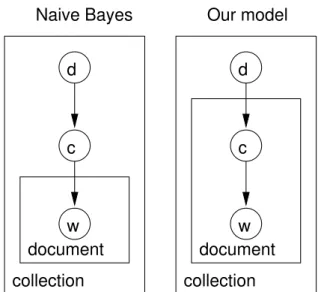
d c w document document w c d Our model Naive Bayes collection collection
Figure 1: Graphical models for Na¨ıve Bayes (left) and for the probabilistic model used here (right).
document P (c = ℓi|di) = 1 and P (c 6= ℓi|di) = 0,
for all i. This greatly simplifies the likelihood, which may now be maximised analytically. Let us introduce |d| =Pwn(w, d) the length of
doc-ument d, |c| =Pd∈c|d| the total size of category
c(using the shorthand notation d ∈ c to mean all documents di such that ℓi = c), and N =Pd|d|
the number of words in the collection. The Max-imum Likelihood (ML) estimates are:
b P(w|c) = 1 |c| X d∈c n(w, d) and Pb(d) = |d| N (3)
Note that in fact only the category profiles b
P(w|c) matter. As shown below, the document probabilityPb(d) is not used for categorising new documents (as it is irrelevant, for a given d).
The ML estimates in eq. 3 are essentially iden-tical to those of the Na¨ıve Bayes categoriser [10]. The underlying probabilistic models, however, are definitely different, as illustrated on figure 1 and shown in the next section. One key dif-ference is that the probabilistic model in eq. 1 is much less sensitive to smoothing than Na¨ıve Bayes.
It should be noted that the ML estimates rely on simple corpus statistics and can be computed in a single pass over the training data. This con-trasts with many training algorithm that rely on
iterative optimisation methods. It means that training our model is extremely efficient.
2.2 Prediction
Note that eq. 1 is a generative model of co-occurrences of words and documents within a
given collection {d1. . . dn} with a set vocabulary
V. It is not a generative model of new docu-ments, contrary to, for example, Na¨ıve Bayes. This means that we can not directly calculate the posterior probability P (d|c) for a new docu-e ment.
We obtain predictions by folding in the new document in the collection. As document de is folded in, the following parameters are added to the model: P (d) and P (c|e d), ∀c. The latter aree precisely the probabilities we are interested in for predicting the category labels. As before, we use a Maximum Likelihood approach, maximis-ing the likelihood for the new document:
e L =X w n(w,d) log P (e d)e X c P(c|d)P (w|c)e (4)
with respect to the unknown parameters P (c|d).e The likelihood may be maximised using a vari-ant of the Expectation Maximisation (EM, [2]) algorithm. It is similar to the EM used for es-timating the PLSA model (see [8, 4]), with the constraint that the category profiles P (w|c) are kept fixed. The iterative update is given by:
P(c|d) ← P (c|e d)e X w n(w,d)e |d|e P(w|c) P cP(c|d)P (w|c)e (5)
The likelihood (4) is guaranteed to be strictly increasing with every EM step, therefore equa-tion 5 converges to a (local) minimum. In the general case of unsupervised learning, the use of deterministic annealing [13] during parame-ter estimation helps reduce sensitivity to initial conditions and improves convergence (cf. [8, 4]). Note however that as we only need to optimise over a small set of parameters, such annealing schemes are typically not necessary at the pre-diction stage. Upon convergence, the posterior probability estimate for P (c|d) may be used as ae basis for assigning the final category label(s) to documentd.e
The way the prediction is obtained sheds some light on the difference between our method and a Na¨ıve Bayes categoriser. In Na¨ıve Bayes, a category is associated to a whole document, and all words from this document must then be gen-erated from this category. The occurrence of a word with a low probability in the category profile will therefore impose an overwhelming penalty to the category posterior P (c|d). By contrast, the model we use here assigns a cate-gory c to each co-occurrence (w, d), which means that each word may be sampled from a different category profile. This difference manifests itself in the re-estimation formula for P (c|d), eq. 5,e which combines the various word probabilities as a sum. As a consequence, a very low proba-bility word will have little influence on the pos-terior category probability and will not impose an overwhelming penalty.
This key difference also makes our model mush less sensitive to probability smoothing than Na¨ıve Bayes. This means that we do not need to set extra parameters for the smoothing process. In fact, up to that point, we do not need to set any extra hyper-parameter for the training or the prediction phase.
As an aside, it is interesting to relate our method to the two paradigms of inductive and
transductive learning [14]. The training phase
seems typically inductive: we optimise a cost function (the likelihood) to obtain one optimal model. Note however that this is mostly a model of the training data, and it does not provide di-rect labelling for any document outside the train-ing set. At the prediction stage, we perform an-other optimisation, this time over the labelling of the test document. This is in fact quite similar to transductive learning. In this way , it appears that our probabilistic model shares similarities with both learning paradigms.
We will now address two important issues of the Anomaly Detection/Text Mining competi-tion that require some extensions to the basic model that we have presented. Multi-label cat-egorisation is addressed in section 2.3 and the estimation of a prediction confidence is covered in section 2.4.
2.3 Multi-class, multi-label categori-sation
So far, the model we have presented is strictly a multi-class, single-label categorisation model. It can handle more than 2 classes (C > 2) but the random variable c indexing the categories takes a single value in a discrete set of C possible cat-egories.
The Anomaly Detection/Text Mining compe-tition is a multi-class, multi-label categorisation problem: each document may belong to multi-ple categories. In fact, although most documents have only one or two labels, one document, num-ber 4898, has 10 labels (out of 22), and 5 docu-ments have exactly 9 labels.
One principled way to extend our model to handle multiple labels per document is to con-sider all observed combinations of categories and use these combinations as single “labels”, as de-scribed eg in [6] (see also [11]). On the competi-tion data, however, there are 1151 different label combinations with at least one associated docu-ment. This makes this approach hardly practi-cal. An additional issue is that considering label combinations independently, one may miss some dependencies between single categories. That is, one can expect that combinations (C4, C5, C10) and (C4, C5, C11) may be somewhat dependent as they share two out of three category labels. This is not modelled by the basic “all model combinations” approach. Although dependen-cies may be introduced as described for example in [6], this adds another layer of complexity to the system. In our case, the number of depen-dencies to consider between the 1151 observed label combinations is overwhelming.
Another approach is to reduce the multiple labelling problem to a number of binary cate-gorisation problems. With 22 possible labels, we would therefore train 22 binary categorisers and use them to take 22 independent labelling deci-sions. This is an appealing and usually successful approach, especially with powerful binary cate-gorisers such as Support Vector Machines [1, 9]. However, it still mostly ignores dependencies be-tween the individual labels (for example the fact that labels C4 and C5 are often observed
to-gether) and it multiplies the training effort by the number of labels (22 in our case).
Our approach is actually somewhat less princi-pled than the alternatives mentioned above, but a lot more straightforward. We rely on a simple threshold a ∈ [0; 1] and assign any new document
e
dto all categories c such that P (c|d) ≥ a. In ad-e dition, as all documents in the training set have at least one label, we make sure thatdealways get assigned the label with the highest P (c|d), evene is this maximum is below the threshold. This threshold is combined with the calculation of the confidence level as explained in the next section.
2.4 Confidence estimation
Another important issue in the Anomaly Detec-tion/Text Mining competition is that labelling has to be provided with an associated confidence level.
The task of estimating the proper probability of correctness for the output of a categoriser is sometimes called calibration [15]. The confidence level is then the probability that a given labelling will indeed be correct, ie labels with a confidence of 0.8 will be correct 80% of the time. Unfortu-nately, there does not seem to be any guarantee that the cost function used for the competition will be optimised by a “well calibrated” confi-dence. In fact there is a natural tension between calibration and performance. Some perfectly cal-ibrated categorisers can show poor performance; Conversely, some excellent categorisers (for ex-ample Support Vector Machines) may be poorly or not calibrated.
Accordingly, instead of seeking to calibrate the categoriser, we use the provided score function, Checker.jar, to optimise a function that outputs the confidence level, given the probability output by the categoriser. In fields like speech recogni-tion, and more generally in Natural Language Processing, confidence estimation is often done by adding an additional Machine Learning layer to the model [3, 5], using the output of the model and possibly additional, external features mea-suring the level of difficulty of the task. We adopt a similar approach, but using a much sim-pler model.
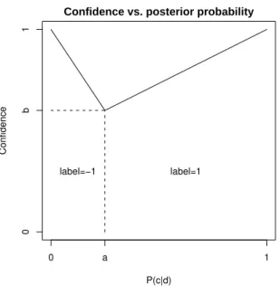
Confidence vs. posterior probability P(c|d) Confidence 0 a 1 0 b 1 label=1 label=−1
Figure 2: The piecewise linear function used to transform the posterior probability into a confi-dence level.
The confidence layer transforms the condi-tional probability output by the model, P (c|d),e into a proper confidence measure by using a piecewise linear function with two parameters (figure 2). One parameter is the probability threshold a, which determines whether a label is selected or not; the second is a baseline confi-dence level b, which determines what conficonfi-dence we give a document that is around the thresh-old. The motivation for the piecewise-linear shape is that it seems reasonable that the confi-dence is a monotonous function of the probabil-ity, ie if two documents de1 and de2 are such that a < P(c|de1) < P (c|de2), then it makes sense to give de2 a higher confidence to have label c than
e
d1. Using linear segments is a parsimonious way to implement this assumption.
Let us note that the entire model, including the confidence layer, relies on two learning pa-rameters, a and b. These parameters may be optimised by maximising the score obtained on a prediction set or a cross-validation estimator, as explained below.
3
Experimental results
We will now describe some of our experiments in more details and give some experimental re-sults, both for the estimated prediction perfor-mance, using only the training data provided for the competition, and for the test performance using the test labels provided after the results were announced.
3.1 Data
The available training data consists of 21519 re-ports categorised in up to 22 categories. Some limited pre-processing was performed by the or-ganisers on the reports, eg tokenisation, stem-ming, acronym expansion and removal of places and numbers. This pre-processing makes it non-trivial for participants to leverage their own in-house linguistic pre-processing. On the other hand, it places contestants on a level-playing field, which put the emphasis on differences in the actual categorisation method, as opposed to differences in pre-processing.1
The only additional pre-processing we per-formed on the data was stop-word removal, us-ing a list of 319 common words. Similar lists are available many places on the internet.
After stop-word removal, documents were in-dexed in a bag-of-word format by recording the frequency of each word in each document.
In order to obtain an estimator of the pre-diction error, we organised the data in a 10-fold cross-validation manner. We randomly re-ordered the data and formed 10 splits: 9 con-taining 2152 documents, and one with 2151 doc-ument. We then trained a categoriser using each subset of 9 splits as training material, as de-scribed in section 2.1, and produced predictions on the remaining split, as described in 2.2. As a result, we obtain 21519 predictions on which we will optimise parameters a and b.
1In our experience, differences in pre-processing
typ-ically yield larger performance gaps than differences in categorisation method.
3.2 Results
The competition was judged using a specific cost function combining prediction performance and confidence reliability. For each category c, we compute the area under the ROC curve, Ac, for
the categoriser. Ac lies between 0 and 1, and
is usually above 0.5. In addition, for each cate-gory c, denote tic∈ {−1, +1} the target label for
document di, yic ∈ {−1, +1} the predicted label
and qic the associated confidence. The final cost function is: Q= 1 C C X c=1 (2Ac− 1) + 1 M M X i=1 qicticyic (6)
Given predicted labels and associated confi-dence, the reference sript Checker.jar provided by the organisers computes this final score. A perfect prediction with 100% confidence yields a final score of 2, while a random assignment would give a final score around 0.
Using the script Checker.jar, on the cross-validated predictions, we optimise a and b us-ing alternatus-ing optimisations along both param-eters. The optimal values are a = 0.24 and b= 0.93, indicating that documents are labelled with all categories that have a posterior proba-bility higher than 0.24, and the minimum confi-dence is 0.93. This is somewhat surprising as it seems like a very high baseline confidence. This suggests that there may be a lot to gain from us-ing a confidence layer that is somewhat more dis-cerning. Using this setting, the cross-validated cost is about 1.691. With the same settings, the final cost on the 7,077 test documents is 1.689, showing an excellent agreement with the cross-validation estimate.
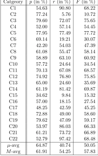
We also measured the performance using some more intuitive metrics. For example, the over-all mislabelling error rate is 7.22%. In addi-tion, table 1 summarises the performance in terms of the standard metrics of precision,
re-call and F-score.2 Over the 22 categories, the
2Precision estimates the probability that a label pro-vided by the model is correct, while recall estimates the probability that a reference label is indeed returned by the model [7]. F-score is the harmonic average of preci-sion and recall.
Catgeory p (in %) r (in %) F (in %)
C1 54.63 90.80 68.22 C2 77.24 5.76 10.72 C3 79.60 72.07 75.65 C4 52.00 57.14 54.45 C5 77.95 77.49 77.72 C6 69.14 19.21 30.07 C7 42.20 54.03 47.39 C8 61.08 55.47 58.14 C9 58.89 63.10 60.92 C10 57.72 24.64 34.54 C11 70.13 67.08 68.57 C12 74.92 76.80 75.85 C13 65.00 24.60 35.69 C14 61.19 81.42 69.87 C15 34.62 9.84 15.32 C16 57.00 18.15 27.54 C17 48.25 42.59 45.25 C18 72.88 49.00 58.60 C19 79.62 47.09 59.17 C20 53.97 86.03 66.33 C21 61.21 73.72 66.89 C22 52.79 97.42 68.48 µ-avg 64.87 40.74 50.05 M-avg 61.91 54.25 57.83 Table 1: Performance of the probabilistic model: precision, recall and F -score for each of the 22 categories, as well as the micro- and macro- av-erages.
micro-averaged precision and recall are 64.9% and 40.7%, respectively, indicating that aroud 40% of reference labels are found by the model, and about 65% of the labels provided by the system were correct. It appears that precision and recall are balanced on most categories, but a few categories (C2, C15, C16, C6) have ter-rible recall. This suggests that having different threshold for different categories may be a way to improve performance.
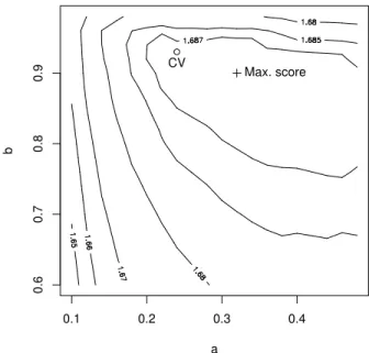
In order to illustrate the sensitivity of the performance to the setting of the two hyper-parameters a and b, we plot the final cost ob-tained for various combinations of a and b, as shown in figure 3. The optimal setting (cross) is in fact quite close to the cross-validation
es-a b 0.1 0.2 0.3 0.4 0.6 0.7 0.8 0.9 Max. score CV
Figure 3: Score for various combinations of a and b. The best (maximum) test score is in-dicated as a cross, the optimum estimated by cross-validation (CV) is a = 0.24 and b = 0.93, indicated by a circle.
timate (circle). In addition, it seems that the performance of the system is not very sensitive to the precise values of a and b. Over the range plotted in figure 3, the maximal score (cross) is 1.6894, less than 0.05% above the CV-optimised value, and the lowest score (bottom left) is 1.645, 2.5% below. This means that any setting of a and b in that range would have been within 2.5% of the optimum.
4
Summary
We have presented the probabilistic model that we used in NRC’s submission to the Anomaly Detection/Text Mining competition at the Text Mining Workshop 2007. This probabilistic model may be estimated from pre-processed, in-dexed and labelled documents with no additional learning parameters, and in a single pass over the data. This makes it extremely fast to train. On the competition data, in particular, the training phase takes only a few seconds. Obtaining pre-dictions for new test documents requires a bit
more calculations but is still quite fast.
The only training parameters we used are re-quired for tuning the decision layer, which selects the multiple labels associated to each documents, and estimates the confidence in the labelling. In the method that we implemented for the compe-tition, these parameters are the labelling thresh-old, and the confidence baseline. They are es-timated by maximising the cross-validated cost function.
Performance on the test set yields a final score of 1.6886, which is very close to the cross-validation estimate. This suggests that despite its apparent simplicity, the probabilistic model provides a very efficient categorisation. This is actually corroborated by extensive evidence on multiple real-life use cases.
The simplicity of the implemented method, and in particular the somewhat rudimentary confidence layer, suggests that there may be am-ple room for improving the performance. One obvious issue is that the ad-hoc layer used for labelling and estimating the confidence may be greatly improved by using a more principled ap-proach. One possibility would be to train multi-ple categorisers, both binary and multi-category, and use the ouptut of these categorisers as input to a more complex model combining this infor-mation into a proper decision associated with a better confidence level. This may be done for example using a simple logistic regression. Note that one issue here is that the final score used for the competition, eq. 6, combines a performance-oriented measure (area under the ROC curve) and a confidence-oriented measure. As a conse-quence, and as discussed above, there is no guar-antee that a well-calibrated classifier will in fact optimise this score. Also, this suggests that there may be a way to invoke multiobjective optimisa-tion in order to further improve the performance. Among other interesting topics, let us men-tion the sensitivity of the method to various ex-perimental conditions. In particular, although we have argued that our probabilistic model is not very sensitive to smoothing, it may very well be that a properly chosen smoothing, or simi-larly, a smart feature selection process, may fur-ther improve the performance. In the context 7
of multi-label categorisation, let us also mention the possibility to exploit dependencies between the classes, for example using an extension of the method described in [12].
References
[1] Cancedda, N., Goutte, C., Renders, J.-M., Cesa-Bianchi, N., Conconi, A., Li, Y., Shawe-Taylor, J., Vinokourov, A., Graepel, T. and Gentile, C. (2002). Kernel Methods for Doc-ument Filtering. The Eleventh Text REtrieval
Conference (TREC 2002), National Institute
of Standards and Technology (NIST).
[2] Dempster, A. P., Laird, N. M., and Rubin, D. B. (1977). Maximum likelihood from in-complete data via the EM algorithm.
Jour-nal of the Royal Statistical Society, Series B,
39(1):1–38.
[3] Gandrabur, S., Foster, G., Lapalme, G. (2006). Confidence Estimation for NLP Ap-plications. ACM Transactions on Speech and
Language Processing, 3(3): 1–29.
[4] Gaussier, E., Goutte, C., Popat, K., and Chen, F. (2002). A hierarchical model for clus-tering and categorising documents.
Proceed-ings of the 24th BCS-IRSG Colloquium on IR Research (ECIR’02), pp. 229–247. Springer.
[5] Gillick, L., Ito, Y. and Young, J. (1997). A Probabilistic Approach to Confidence Estima-tion and EvaluaEstima-tion. ICASSP ’97:
Proceed-ings of the 1997 IEEE International Confer-ence on Acoustics, Speech, and Signal Process-ing (ICASSP ’97)-Volume 2, pp. 879–882.
[6] Goutte, C. and Gaussier, E. (2004). Method for multi-class, multi-label categorization us-ing probabilistic hierarchical modelus-ing. US Patent 7,139,754 (granted Nov. 21, 2006).
[7] Goutte, C. and Gaussier, E. (2005). A Probabilistic Interpretation of Precision, Re-call and F-Score, with Implication for Evalua-tion. Advances in Information Retrieval, 27th
European Conference on IR Research (ECIR 2005), pp. 345-359. Springer.
[8] Hofmann, T. (1999). Probabilistic latent se-mantic analysis. Uncertainty in Artificial
In-telligence (UAI’99), pp. 289–296.
[9] Joachims, T. (1998). Text Categorization with Suport Vector Machines: Learning with Many Relevant Features. ECML ’98:
Proceed-ings of the 10th European Conference on Ma-chine Learning, pp. 137–142.
[10] McCallum, A. and Nigam, K. (1998). A Comparison of Event Models for Naive Bayes Text Classification. AAAI/ICML-98
Work-shop on Learning for Text Categorization, pp.
41–48.
[11] McCallum, A. (1999). Multi-Label Text Classification with a Mixture Model Trained by EM. AAAI’99 Workshop on Text
Learn-ing.
[12] Renders, J.-M., Gaussier, E., Goutte, C., Pacull, F. and Csurka, G. (2006). Catego-rization in multiple category systems.
Ma-chine Learning, Proceedings of the Twenty-Third International Conference (ICML 2006),
pp. 745–752.
[13] Rose, K., Gurewwitz, E., and Fox, G. (1990). A deterministic annealing approach to clustering. Pattern Recogn. Letters, 11(9):589– 594.
[14] Vapnik, V. N. (1998). Statistical Learning
Theory. Wiley.
[15] Zadrozny, B. and Elkan, C. (2001). Obtain-ing calibrated probability estimates from deci-sion trees and naive Bayesian classifiers.
Pro-ceedings of the Eighteenth International Con-ference on Machine Learning (ICML’01).