Loading due to interaction of waves with colinear and oblique currents

Publisher’s version / Version de l'éditeur: Ocean Engineering, 81, pp. 1-11, 2014-03-05

READ THESE TERMS AND CONDITIONS CAREFULLY BEFORE USING THIS WEBSITE. https://nrc-publications.canada.ca/eng/copyright

Vous avez des questions? Nous pouvons vous aider. Pour communiquer directement avec un auteur, consultez la première page de la revue dans laquelle son article a été publié afin de trouver ses coordonnées. Si vous n’arrivez pas à les repérer, communiquez avec nous à PublicationsArchive-ArchivesPublications@nrc-cnrc.gc.ca.

Questions? Contact the NRC Publications Archive team at

PublicationsArchive-ArchivesPublications@nrc-cnrc.gc.ca. If you wish to email the authors directly, please see the first page of the publication for their contact information.

NRC Publications Archive

Archives des publications du CNRC

This publication could be one of several versions: author’s original, accepted manuscript or the publisher’s version. / La version de cette publication peut être l’une des suivantes : la version prépublication de l’auteur, la version acceptée du manuscrit ou la version de l’éditeur.

For the publisher’s version, please access the DOI link below./ Pour consulter la version de l’éditeur, utilisez le lien DOI ci-dessous.

https://doi.org/10.1016/j.oceaneng.2014.02.005

Access and use of this website and the material on it are subject to the Terms and Conditions set forth at Loading due to interaction of waves with colinear and oblique currents

Zaman, M. Hasanat; Baddour, Emile

https://publications-cnrc.canada.ca/fra/droits

L’accès à ce site Web et l’utilisation de son contenu sont assujettis aux conditions présentées dans le site LISEZ CES CONDITIONS ATTENTIVEMENT AVANT D’UTILISER CE SITE WEB.

NRC Publications Record / Notice d'Archives des publications de CNRC: https://nrc-publications.canada.ca/eng/view/object/?id=6983cda3-0601-4456-a145-4e26917faa74 https://publications-cnrc.canada.ca/fra/voir/objet/?id=6983cda3-0601-4456-a145-4e26917faa74

LOADING DUE TO INTERACTION OF WAVES WITH COLINEAR AND OBLIQUE CURRENTS

M. Hasanat Zaman and Emile Baddour

National Research Council Canada Arctic Ave., PO Box 12093 St. John’s, NL, A1B 3T5, Canada

E-mail: Hasanat.Zaman@nrc-cnrc.gc.ca

Abstract

A study on the loading of an oblique surface wave and a surface current field on a fixed vertical slender cylinder in a 3D flow frame is illustrated in the present paper. The three dimensional expressions describing the characteristics of the combined wave-current field in terms of mass, momentum and energy flux conservation equations are formulated. The parameters before the interaction of the oblique wave-free uniform current and current-free wave are used to formulate the kinematics of the flow field. These expressions are also employed to formulate and calculate the loads imparted by the wave-current combined flow on a bottom mounted slender vertical cylinder. In the present study two different situations are assumed where current is uniform over depth and also acting over a layer of fluid that extends from the free surface to a specified finite depth. In this paper we extend the approach considered in Zaman and Baddour (2004) for the wave-current analysis. Morison et al (1950) equation is deployed for the load computations in all cases. The above models are utilized to compute the loads and moments on a slender cylinder for a wave with varying range of incidence current field.

Keywords: 3D wave-current field, superposition model, wave-current loading, moment

1. Introduction

Water motion in the sea is a mixture of wave and current of different forms. The coexistence of waves and currents, their interaction and consequently their loadings on any ocean structure are very important issues for ocean engineers and related scientists to study the stability of the ocean structures. In order to estimate the performance of any ocean structure it is very important for the designer to account for the loading effects resulting from the interaction of a combined wave-current field with any ocean structure.

Longuet-Higgins and Stewart (1960 and 1961), Whitham (1962) derived theoretical expressions for the changes in sea level and other linear and nonlinear characteristics of 2D wave trains by considering momentum flux. Kemp and Simons (1982 and 1983) described the wave-current interactions for following and reverse current. Zaman and Togashi (1996) described their experimental results for interaction of monochromatic wave with favorable and adverse currents over a parabolic bottom structure. Zaman et al (2008) compared their theoretical and experimental results for interacted wave-current field over a parabolic bottom structure. Zaman and Baddour (2010) described the interaction of the wave with collinear current. Hedges and Lee (1991) showed that an equivalent uniform current could replace a depth varying current.

In the present model formulation it is assumed that the flow fields are irrotational and inviscid. This allows the estimation of the flow characteristics needed in a Morison et al equation context. Velocity potentials are adopted to express the oblique flow fields in 3D

for: (i) a wave field in the absence of current; (ii) a current field in the absence of wave and (iii) the wave-current combined field after the interaction of both a current-free wave and a wave-free current. These three distinct flow fields are first introduced for collinear flows in Baddour and Song (1990a and 1990b) and extended in 3D in Zaman and Baddour (2003). Zaman and Baddour (2004) showed a comparison of the obtained results due to the present model to those obtained using three other numerical models being used in the offshore industry. These results are shown for a wide range of the normalized current parameters.

For the computation of the parameters of the wave-current field, we have developed three-dimensional expressions describing the characteristics of the combined flow in terms of mass, momentum and energy transport conservation equations and the given before-interaction parameters of a wave-free uniform current and current-free wave. These equations are efficient in describing the combined wave-current field parameters. The relations obtained in satisfying the conservation of mass, momentum, energy flux and a dispersion relation generate a system of nonlinear equations that are solved to evaluate the sought-for wave-current flow parameters, namely, the free surface wave height, wavelength, current-like term, mean water depth and combined wave-current field direction for a non-collinear case after the interaction. In other words due to the presence of the current the location of the mean water level as well as other parameters of the combined wave-current field will change after the interaction such that to satisfy the conservation equation mentioned above. The concept was generalized for oblique waves in Zaman and Baddour (2002). The obtained model also encompasses the 2D case and is applicable to a current-free or a wave-free flow with appropriate boundary conditions.

In the present computation, we first calculate different parameters of the interacted wave-current field and then use those parameters to calculate the loads imparted by the fluid on a bottom mounted slender vertical cylinder representing a typical element of an offshore structure. For surface currents we also compute moments for current along with loads about the bottom of the cylinder. In this paper the comparisons of computed loads on a slender cylinder by combined wave-current flow field and by superposing wave and current field is shown and discussed. The load computation uses Morison et al (1950) equation with appropriate drag and mass coefficients given by Iwagaki et al (1983). See also for example Chakrabarti (1987) and Sarpkaya and Isaacson (1981).

2. Properties of the 3D Wave-Current Field

2.1 Theory

We assume that a current-free monochromatic plane surface wave of wavelength Lo

(=2ko), wave height Ho (=2ao) and period T propagates over a water body of depth do in

the direction given by Nw and that independently there exists a horizontal uniform wave-free current Uo over the same water depth do in the direction Nc

 .

When these two plane fields meet, see Fig. 1, a plane of combined wave-current field develops in the direction N, with a new set of unknown parameters namely, wavelength L

(=2k), wave height H (=2a), current parameter U and depth d. These unknown parameters together with direction N are required to be computed from a system of

conservation equations described in the next sections. We first formulate the potential of a wave-current field in a direction N.

Fig. 1 shows the plan view of the computational domain with O the origin of the 3D inertial frame. The x and y axes subtend the horizontal plane, and z the vertical axis is perpendicular at O to both x and y, and points towards the reader. The unit vectors Nc, Nw

and N denote the directions of the wave-free current, current-free wave and wave-current plane fields, respectively. The unit vector S is normal to N.

Fig.1 Wave-free current, current-free wave and wave-current fields relative directions Assuming inviscid and incompressible fluid flows we posit that the result of the interaction between a current-free wave with a wave-free current exists and is here called a wave-current flow field in the N direction. A velocity potential describes this field is given by the following expression to second order in the surface undulation amplitude:



 



        cosh ( )sin( ) sinh ) , , , ( 1 U k k d z k x t kd k a x U t z y x        





cosh2 ( )sin2( ) ( ) coth 4 1 2 sinh 1 2 3 3 1 2 a k kd U k k d z k x t O k a a kd k            _{ }     _ (1) where U U(Ux,Uy) 

 is the current parameter and k k(kx_,ky) 

 is the wave number whose related vector is normal to the surface undulation front in the wave-current field and lies in the horizontal x-y plane,  is the angular frequency, a the amplitude of the surface undulation in the wave-current field, C the celerity, d the mean water depth, t the time,

) , (x y

x the horizontal position vector of a point in the field and z is the vertical axis measured vertically upward from the still water level. The first and second order surface elevation amplitudes are given by a₁ and a₂, respectively. See for example Dean and Dalrymple (1992) for the first order 2D collinear case, and Baddour and Song (1990b) for the second and higher order collinear case.

The relation of the wave number and the angular frequency of the combined wave-current field is given by the following Doppler relation:

r

k

U 

   (2)

where the relative angular frequency in the above equation is described by the following equation: i j c  w_ Wave-current field z  x y N S w N Wave field Current field O c N k

kd gk

r  tanh

 (3)

The dispersion relation for the combined wave-current field is hence:



 Uk



 gktanhkd (4)

The instantaneous free surface elevation  is to first order in amplitude a expressed as: ) ( ) cos(k x t O a2 a         (5) 2.2 Fluid kinematics

The particle velocity components in the x, y and z direction in the combined wave-current field (equations 6 to 8), wave-current-free wave field (equations 9 to 11) and wave-free current field (equations 12 to 14) are obtained as:

) cos( ) ( cosh sinh 1 _{k d z k x t} k k kd a U u r x x wc x   _{  }     ) ( 2 cosh coth 2 1 2 sinh 2 2 1 2 a k kd k d z a k k kd x r      _   ) ( ) ( 2 cos kx t O k3a3     (6) ) cos( ) ( cosh sinh 1 t x k z d k k k kd a U u y r y wc y          ) ( 2 cosh coth 2 1 2 sinh 2 2 1 2 a k kd k d z a k k kd y r         ) ( ) ( 2 cos kx t O k3a3     (7) ) sin( ) ( sinh sinh 1 t x k z d k kd a uzwc r         ) ( 2 sinh coth 2 1 2 sinh 2 ₂ 1 2 a k kd k d z a kd r         ) ( ) ( 2 sin kx t O k3a3     (8) ) cos( ) ( cosh sinh 1 _{k d z k x t} k k kd a uw r x x         ) ( 2 cosh coth 2 1 2 sinh 2 2 1 2 a k kd k d z a k k kd x r         ) ( ) ( 2 cos kx t O k3a3     (9) ) cos( ) ( cosh sinh 1 _{k d z k x t} k k kd a uw r y y         ) ( 2 cosh coth 2 1 2 sinh 2 2 1 2 a k kd k d z a k k kd y r        

) ( ) ( 2 cos kx t O k3a3     (10) ) sin( ) ( sinh sinh 1 t x k z d k kd a u_zw  r   ) ( 2 sinh coth 2 1 2 sinh 2 2 1 2 a k kd k d z a kd r         ) ( ) ( 2 sin kx t O k3a3     (11) x c x U u  (12) y c y U u  (13) 0  c z u (14)

where superscripts w, c and wc in the above equations, stand for the quantities in the pre-interaction current-free wave field, wave-free current field and in the post-pre-interaction wave-current field, respectively.

The corresponding acceleration components in the x, y and z directions in the combined wave-current field (equations 15 to 17), current-free wave field (equations 18 to 20) and wave-free current field (equations 21 to 23) are evaluated as:

) sin( ) ( cosh sinh 1 t x k z d k k k kd a awc r x x          ) ( 2 cosh coth 2 1 2 sinh 4 ₂ 1 2 a k kd k d z a k k kd x r          ) ( ) ( 2 sin kxt O k3a3 (15) ) sin( ) ( cosh sinh 1 t x k z d k k k kd a awc_y  r y   ) ( 2 cosh coth 2 1 2 sinh 4 2 1 2 a k kd k d z a k k kd y r _         ) ( ) ( 2 sin kxt O k3a3 (16) ) cos( ) ( sinh sinh 1 t x k z d k kd a awc r z           ) ( 2 sinh coth 2 1 2 sinh 4 2 1 2 a k kd k d z a kd r _         ) ( ) ( 2 cos kxt O k3a3 (17) ) sin( ) ( cosh sinh 1 _{k d z k x t} k k kd a aw r r x x         

) ( 2 cosh coth 2 1 2 sinh 4 ₂ 1 2 a k kd k d z a k k kd x r r          ) ( ) ( 2 sin kxt O k3a3 (18) ) sin( ) ( cosh sinh 1 _{k d z k x t} k k kd a aw r r y y          ) ( 2 cosh coth 2 1 2 sinh 4 ₂ 1 2 a k kd k d z a k k kd y r r          ) ( ) ( 2 sin kxt O k3a3 (19) ) cos( ) ( sinh sinh 1 _{k d z k x t} kd a a_zw  rr   ) ( 2 sinh coth 2 1 2 sinh 4 2 1 2 a k kd k d z a kd r r          ) ( ) ( 2 cos kxt O k3a3 (20) 0  c x a (21) 0  c y a (22) 0  c z a (23)

The pressure distribution in the wave-current field to second order is obtained from the dynamic free surface boundary condition as:





cos( ) cosh ) ( cosh 1 ) ( 2 cosh 2 sinh 2 2 t x k kd z d k ga z d k kd k ga gz P        kd k ga kd z d k kd k ga 2 sinh 2 sinh ) ( 2 cosh 2 sinh 2 3 2 2 2          (24)

2.3 Derivation of mass, momentum and energy flux equation

We can obtain the mass flux of the combined wave-current field along the zN

vertical plane through the following relation up to second order in amplitude a (for details

see Zaman and Baddour, 2010):





    d dz Q d x y wc

 

    2 0 2 1 (25) ) ( coth 2 3 3 2 a k O kd k k U C k a U d Qwc _        _         _  (26)

The corresponding momentum flux of the combined wave-current field along the same

N

z  plane is given as follows:



 



    d dz t z y x t z y x t z y x P M d x y wc

 

      2 0 2 2_{( , , , ) ( , , , )} ) , , , ( 2 1 (27) ) ( 2 1 2 1 2 2 sinh 2 2 1 2 1 3 3 2 2 2 _{O k a} gd U gd k U kd kd ga M r wc _                     _           (28)

In a similar fashion the net energy flux of the combined wave-current field in the direction of flow in the zN plane is expressed as:





gz dzd j x y P E d x y z j wc j : , 2 2 1 2 0 2 2 2 _{ }              _{   } 

 

       (29) k k k k U C kd kd ga a kd gk U d U a U g E r wc                            _   2 sinh 2 1 4 2 sinh 2 2 2 2 2 2    ) ( ) ( 2 4 3 3 2 2 a k O U k k U U ga r      _{ }         (30) where k kN and U U N.

2.4 Conservation equation and numerical method

The following two sets of conservation equations for mass, momentum and energy flux in the N and S directions, respectively obtained when the time averages of the flux parameters of the current-free wave field, wave-free current field and wave-current field are considered: N N Q N N Q N N Qw w  c c   wc   (31) N N M N N M N N Mw w  c c    wc   (32) N N E N N E N N Ew w  c c  wc   (33) 0    S Q N S N Qw w  c c  (34) 0    S M N S N Mw w  c c  (35) 0    S E N S N Ew w  c c  (36)

The directional vectors are denoted by the following expression:

j i Nwcosw sinw  (37) j i Nc cosc sinc  (38) j i N cos sin  (39) j i Ssin cos  (40)

and w

N and c

N are the given wave and current directions; N is the final direction of the combined wave-current field and S is the direction normal to N. w and c are the given current-free wave direction and wave-free current direction prior to interaction and  is the final direction of the combined wave-current field after interaction with the x-horizontal axis.

The vector relationships mentioned in the equations (37) to (40) are invoked and properly used in the derivation of the conservation of mass, momentum and energy equations in the respective sections.

2.5 Variables declaration

The known and unknown parameters used in this formulation are normalized and defined in the following way:

Normalized known parameters:

2 2 o o d a A ; o o C U B ; o o d L D ;  (not normalized) (41)

Normalized unknown parameters:

o d d W  ; o C U X  ; o L L Y2  ; 2 2 o d a Z  ; tan (42) 2.6 Dispersion relation

The normalized dispersion relation (equation 4) for the combined wave-current field can be rewritten in the following form:



tanh(2 / 2)coth(2 / )



1/2 0 2 _{  } D DY W Y X Y   (43) 2.7 Conservation of mass

The mean rate of transfer of mass across a vertical plane due to the current-free wave field, wave-free current field and combined wave-current field can be written from equation (26) in the following forms:

w o o o o o w w w _{Q N} a _{C k d k N} Q  coth( )  2 2    (44) c o o c c c _{Q N d U N} Q     (45) N k k k U C kd a N dU N Q Qwc wc                    coth( ) 2 2   (46)

Inserting equations (44) to (46) into equation (31) and after normalization the following equation would be obtained to express the conservation of mass in the N

direction:

DWX DB

D

Acoth(2/ )cos(w) cos(c ) 



coth(2 / )coth(2 / )



2 0 1 2 _  W DY D Y Z _{ }  (47)

From equation (34) the conservation of mass equation in the S



direction could be obtained in the following way:

coth(2 / )sin( w ) sin( c ) 0

A D DB

        (48)

2.8 Conservation of momentum

The mean rate of transfer of momentum due to the current-free wave field, wave-free current field and combined wave-current field can be written using equation (28) in the following way: w o o o o o o w w _{gd N} d k d k ga N M                    2 2 2 1 ) 2 sinh( 2 2 1 2 1_{ } (49) c o o c c_{N d U N} M    2  (50) N gd U gd k U kd kd ga N M r wc                                        2 2 2 ₁ 2 2 1 2 ) 2 sinh( 2 2 1 2 1 _   (51)

Substituting equations (49) to (51) into equation (32) and after normalization the conservation of the momentum equation in the N direction would be obtained as follows:

) cos( ) / 2 tanh( ) cos( ) / 2 cosh( ) / 2 sinh( / 2 2 1 1 2          _{  }               w D_{B D} c D D D A            ) / 2 cosh( ) / 2 sinh( / 2 2 1 2 2 2 2 DY W DY W DY W Z W   



tanh(2 / )coth(2 / )



tanh(2 / ) 0

2 2  2   D W DY DW X D Y XZ _    (52)

From equation (35) the normalized conservation of momentum equation in the S

direction could be obtained in the following form:

1 2 / 1 sin( ) 2 sinh(2 / ) cosh(2 / ) w D A D D  _{ }                0 ) sin( ) / 2 tanh( 2 _{ }      B D c D (53) 2.9 Conservation of energy

The mean rate of transfer of energy due to the current-free wave field, wave-free current field and combined wave-current field can be written using equation (30):

w o o o o o o ro o w w N k k d k d k C ga N E            ) 2 sinh( 2 1 4 2  (54) c o c c_N d U _UN E    2 2   (55) N k k k k U C kd kd ga N a kd gk U d U N a U g N Ewc _r                           _                   ) 2 sinh( 2 1 4 ) 2 sinh( 2 2 2 2 2 2    N U k k U U ga r           _{ }  2 2 ( ) 2 4  (56)

Introducing equations (54) to (56) into equation (33) and after normalization the conservation of the energy equation in the N direction would be obtained as:

3

2 /

1 cos( ) tanh(2 / ) cos( ) 2

sinh(2 / ) cos(2 / ) w c D D A D B ZX D D  _{    }               X DY W DY W D Y D Z X D DW           ) / 2 cosh( ) / 2 sinh( ) / 2 tanh( 1 2 ) / 2 tanh( 2 2 2 2 2 2      





                   Y W DY D X DY W DY W DY W Z 2 1 2 2 2 2 ) / 2 coth( ) / 2 tanh( ) / 2 cosh( ) / 2 sinh( / 2 1     



tanh(2 / )coth(2 / )



0 3 2 1 2 2   D W DY Y Z X _{ } (57)

Finally, from equation (36) the normalized conservation of energy equation in the S

direction could be obtained in the following form:

3

2 /

1 sin( ) tanh(2 / )sin( ) 0

sinh(2 / ) cos(2 / ) w c D DB A D D D  _{    }               (58)

2.10 Forms of Morison’s equations

The forms of Morison’s equations (Morison et al, 1950) used in the load computations are given by the following expressions (Chakrabarti, 2005):

Dt u D A C F_{I M M}    (59) u u A C F_D  _{D D} (60) where 2 4 D AM   ,AD ₂ D 

 ; CM and CDare inertia and drag coefficients,  the fluid

density and D is the diameter of the cylinder. D Dttu xv yw z is the time derivative, where ux, uy and uz are the particle velocity components of u



in the x, y and

The coefficients CM and CD are obtained for a specific Keulegan-Carpenter number

(KC) from the curve proposed by Iwagaki et al (1983). The total load F_t is then obtained from the summation of the inertia and the drag forces as:

D I

t F F

F     (61)

where F_I is the force due to inertia and FD



is the force due to drag.

The KC number (Keulegan-Carpenter parameter) that is a measure of the importance of drag force effect is defined by the following equations:

D T u KC max /   (62)

where T is the wave period and umax



is the maximum particle velocity in the x, y and z directions, respectively.

3. Numerical simulation

3.1 Computational procedure

Equations (43), (47), (52) and (57) and, equations (48), (53) and (58) are the required two sets of equations for the evaluations of the properties of the combined wave-current field that results when a current-free wave and a wave-free current interact in a 3D flow field.

At the beginning of the computation the direction of the combined wave-current field is necessary. An iterative solution of any one of the three equations (48), (53) or (58) will give the direction of the combined wave-current field after the interaction. Once the direction of the combined flow is estimated then the system of the nonlinear equations (43), (47), (52) and (57) can be solved iteratively for the required variables W, X, Y and Z. When the variables are known then the computations of the unknown combined wave-current field parameters, a, k, d and U are carried out.

A Newton iterative method has been utilized in this study. For a given wave with parameters ao, ko, do and current velocity Uo, the computation of the parameters a, k, d and U of the combined wave-current field are carried out from the above equations with a

suitable initial guess of the unknowns necessary for iteration to start. If it is assumed that 0

   

_{w c} then the above 3D numerical model becomes a 2D wave-current model discussed in Zaman and Baddour (2006) and Zaman et al (2008).

3.2 Computational environment

Maple-XII is a symbolic programming language using Windows environment. It is used for implementing Newton’s algorithm for the numerical solution of the conservation equations together with the dispersion relation. Maple is a system for mathematical computations that can handle symbolic, numeric and graphical procedures in a simplified way. Maple is easily adaptable for those who have experience in other programming computer languages. An important property of Maple is that all the algebraic routine operations in the system are implemented using high-level user language. The basic system, or kernel, is sufficiently compact and efficient to be practical for use in a shared environment or on a personal computer with as little as 2MB of RAM. One of the advantages of Maple is that the user can see an equation in its expanded mathematical format on the monitor while it is taking part in the computations.

4. Implementation of 2D and 3D models for uniform current extended

from free surface to bottom

Two different numerical models have been used in this study where 2D and 3D Models are our proposed model and, S2D and S3D are superposition models. In 2D and 3D Models, the total load is calculated from the kinematics of the combined wave-current field. In this case equations (6) to (8), equations (15) to (17) and equations (43), (47), (52) and (57) will predict the wave-current parameters and equation (61) would produce the total load exerted on the cylinder by the combined wave-current field.

S2D and S3D are superposition models where the individual components of the loads on the cylinder, due to a current-free wave and a wave-free current, are separately evaluated and a summation of both loads is then made. Equations (9) to (11), equations (18) to (20) and equations (43), (47), (52) and (57) would be used to compute the kinematics of the current-free wave field and then equations (61) is deployed for the computation of the load exerted by the current-free wave. Again when the kinematics of the current field are known from equations (12) to (14), equations (21) to (23) and equations (43), (47), (52) and (57) then equations (61) will give the load due to the wave-free current field. An appropriate summation is then made to obtain the total load.

Table 1. Description of computational method Models Kinematics Load computed 2D Model

3D Model

for combined wave and current field

for combined wave and current field

S2D Model S3D Model

for current-free wave field for wave-free current field

for current-free wave field + for wave-free current field

4.1 Case study: Comparisons of loads by 2D and 3D models with corresponding S2D and S3D models

As an example, the established models have been applied for the computation of loads for a collinear or 2D case and for an oblique or 3D case. For both examples, it is assumed that a monochromatic current-free surface wave interacts with a normalized wave-free uniform current Uo/Co varying over the range of an opposite current to a range of following

currents. The wave and current parameters used in this study are shown in Table 2. Subscript 0 denotes a value of a parameter before interaction. The diameter of the cylinder is 35cm in all computations.

Table 2. Computational parameters

Parameters 2D Model 3D Model

Uo/Co (Maximum opposing) -0.20 -0.20

Uo/Co (Maximum following) 0.572 1.359

Ho/Lo 0.01 0.01

do/Lo 2.0 2.0

Wave incident direction 0 o 10o

In this comparison Table-2 is used for the computational parameters. In the table Ho and Lo are the current-free wave height and wavelength, respectively.

4.1.1 Load computation by the 2D and S2D models

Figs. 2 and 3 show simple comparison of the wave heights and wavelengths, respectively obtained by the 2D Model, experiments by Zaman and Togashi (1996) and experiments by Thomas (1981). However, in Fig. 3 the experimental data of wavelengths by Zaman and Togashi is not available. In this case the predicted and observed wave height

H is normalized by the current-free wave height, Ho and the predicted and observed

wavelength L is normalized by the current-free wavelength Lo. A good match of the model

results with experiments is observed.

Fig. 2 Comparison of the wave heights obtained from the 2D numerical model with experiments

Fig. 3 Comparison of the wavelengths obtained from the 2D numerical model with experiments 3.0 2.5 2.0 1.5 1.0 0.5 0.0 H / H o 0.6 0.5 0.4 0.3 0.2 0.1 0.0 -0.1 -0.2 U o /Co 2D Model

Experiment by Zaman and Togashi (1996) Experiment by Thomas (1981) 3.0 2.5 2.0 1.5 1.0 0.5 0.0 L / L o 0.6 0.5 0.4 0.3 0.2 0.1 0.0 -0.1 -0.2 U o /Co 2D Model Experiment by Thomas (1981)

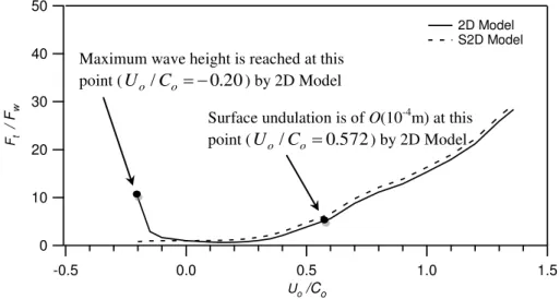
Descriptions of maximum and minimum loads obtained by the above two models for 2D collinear, non-oblique case are given in Fig. 4 and Fig. 5, respectively. In the 2D case we have found that the monochromatic wave height is of O(10-4m) in 2D Model when normalized current parameter reaches the value Uo/Co = 0.572 for the case of a wave with a

following current. For the case when wave and current are in the opposite direction the maximum wave height is reached at Uo/Co = -0.20. Maximum wave height is reached due

to wave blocking. At this point wave steepness exceeds the allowable breaking value (~0.14) and the numerical model is stopped.

50 40 30 20 10 0 Ft / F w 1.5 1.0 0.5 0.0 -0.5 U_o /C_o 2D Model S2D Model

Fig. 4 Normalized maximum exerted loads computed by 2D Model and S2D Model

50 40 30 20 10 0 -10 -20 Ft / F w 1.5 1.0 0.5 0.0 -0.5 U_o /C_o 2D Model S2D Model

Fig. 5 Normalized minimum exerted loads computed by 2D Model and S2D Model. These limits are shown in Fig. 4 and in Fig. 5 by a black-circle. The analyses and comparisons of loads for 2D non-oblique case are made at these two points, that is, when

Uo/Co = 0.572 and Uo/Co = -0.20. In the figures and tables Ft stands for the total load due to

combined wave-current field or due to wave-free current field and Fw describes the load

due to current-free wave field. In Figs. 4 and 5, it may be observed that when waves and

Surface undulation is of O(10-4m) at this point (Uo/Co 0.572) by 2D Model

Surface undulation is of O(10-4m) at this point (U_o/C_o 0.572) by 2D Model Maximum wave height is reached at this point (Uo/Co 0.20) by 2D Model

Maximum wave height is reached at this point (Uo/Co0.20) by 2D Model

currents are in the same direction, that is, Uo/Co is positive, then for the given, before

interaction wave and current conditions, the maximum load obtained at Uo/Co = 0.572 by

the S2D Model is 17.79% [%={2D Model – S2D Model}/ 2D Model*100] larger than that obtained by 2D Model.

Again for the minimum load shown in Fig. 5, S2D Model yields 17.82% smaller load than 2D Model. The above results are summarized in Table 3. A plus sign or a minus sign in the bracket after the percentage value means whether the respective model returns a greater or a smaller load compare to 2D Model.

Table 3. Loads for 2D case: wave with following current

Uo/Co Ft/Fw * % 2D Model 0.572 5.614554 S2D Model 0.572 6.613573 17.79 (+) Uo/Co Ft/Fw ** % 2D Model 0.572 5.614183 S2D Model 0.572 4.613573 17.82 (-)

*Normalized maximum load, **Normalized minimum load

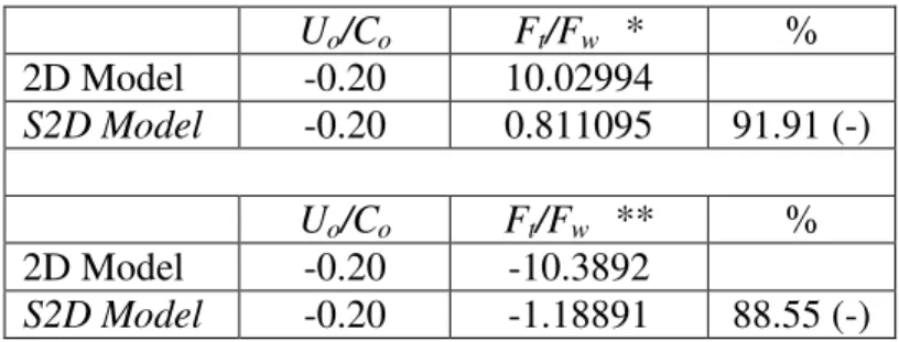
On the other hand when wave and current are in opposite directions the maximum load obtained at Uo/Co = -0.20 by S2D Model is 91.91% smaller than the load obtained by

2D Model. Again for the minimum load, S2D Model yields 88.55% smaller load than 2D Model. Table 4 captures the above findings.

Table 4. Loads for 2D case: wave with opposing current

Uo/Co Ft/Fw * % 2D Model -0.20 10.02994 S2D Model -0.20 0.811095 91.91 (-) Uo/Co Ft/Fw ** % 2D Model -0.20 -10.3892 S2D Model -0.20 -1.18891 88.55 (-)

The possibility of such behavior is that in S2D Model, the wave heights and the wavelengths are not affected by the interaction since wave and current kinematics are computed separately using before interaction parameters. That is no action of wave on current and vice versa is accounted for. On the other hand, in 2D Model, the kinematics is computed from the combined wave-current field where the interaction of wave and current is taken into account. This produces a significant change in wave heights and wavelengths. It is evident that a following current reduces the wave heights and increases the wavelengths. A substantial increase in wave heights and decrease in wavelengths are observed in the waveform for the case of an opposite current. So for the case of a wave interacting with a reverse current, the increase in the wave heights is considered to be responsible for the rapid increase of the loads in a combined wave-current field.

It is important to mention here that when wave and current are in the same direction the wave height reduces with current and disappears when the current is strong enough to eliminate the wave amplitude from the combined wave-current field. In the absence of wave the model is still capable to compute the loading imparted by the wave-free current field. The continuation of the solid line (for 2D Model) in the figures after the black-circle, describes the loading due to wave-free current field in this case.

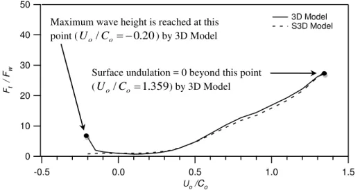
4.1.2 Load computation by the 3D and S3D models

For the oblique interaction cases the above mentioned wave and current conditions are used (as shown in Table 2) and in addition, it is assumed that the wave enters the computational domain at an oblique angle of 10o degree, while the current is at an angle of 15o with the positive direction of the x-axis.

50 40 30 20 10 0 Ft / F w 1.5 1.0 0.5 0.0 -0.5 U_o /C_o 3D Model S3D Model

Fig.6 Normalized maximum exerted loads computed by 3D Model and S3D Model

50 40 30 20 10 0 -10 -20 Ft / F w 1.5 1.0 0.5 0.0 -0.5 U_o /C_o 3D Model S3D Model

Fig. 7 Normalized minimum exerted loads computed by 3D Model and S3D Model Figs. 6 and 7 demonstrate the comparison between the maximum and minimum loads obtained by the above two models in the oblique 3D field. In the 3D oblique case, the

Surface undulation = 0 beyond this point (Uo/Co1.359) by 3D Model

Maximum wave height is reached at this point (U_o/C_o 0.20) by 3D Model Surface undulation = 0 beyond this point

(Uo/Co 1.359) by 3D Model

Maximum wave height is reached at this point (Uo/Co 0.20) by 3D Model

analyses and comparisons of loads are also made at two points, at Uo/Co = 1.359 when

surface undulation is of O(10-4m) for a wave with a following current and at Uo/Co = -0.20

when the wave is in opposite direction of the current. In Figs. 6 and 7, it may be perceived that when waves and currents are in the same direction, that is, Uo/Co is positive, then for

the given wave and current parameters the maximum load obtained at Uo/Co = 1.359 by

S3D Model is 0.70% [%={3D Model - S3D Model}/3D Model*100] smaller than that obtained by 3D Model. Again for minimum load, S3D Model yields 0.96% larger load than 3D Model. Table 5 summarizes the above results.

Table 5. Loads for 3D case: wave with following current

Uo/Co Ft/Fw * % 3D Model 1.359 26.28006 S3D Model 1.359 26.08588 0.700 (-) Uo/Co Ft/Fw ** % 3D Model 1.359 23.85693 S3D Model 1.359 24.08588 0.960 (+)

On the other hand, when wave and current are in opposite directions the maximum load obtained at Uo/Co = -0.20 by S3D Model is 86.86% smaller load than 3D Model.

Again for minimum load, S3D Model yields 82.0% smaller load than 3D Model. These results are summarized in Table 6. For the 3D oblique case we have not proceeded after

Uo/Co = 1.359 since wave height at this current becomes negligible.

Table 6. Loads for 3D case: wave with opposing current

Uo/Co Ft/Fw * % 3D Model -0.20 6.219178 S3D Model -0.20 0.816624 86.86 (-) Uo/Co Ft/Fw ** % 3D Model -0.20 -6.57534 S3D Model -0.20 -1.18338 82.00 (-)

5. Implementation of the 2D and 3D model for layered surface current

In this study it is assumed that current is uniform and acting over a layer of fluid that extends from the free surface to a specified finite depth. The definition sketch of the domain is shown in Fig. 8. In this computation, we calculate the loads imparted by the fluid on a bottom mounted slender vertical cylinder representing a typical element of an offshore structure. The load computation uses Morison’s equation with appropriate drag and mass coefficients. See for example Chakrabarti (1987, 2005) and Sarpkaya and Isaacson (1981).

Fig. 8 Schematic view of 2D wave-free current and current-free wave field before and after interaction.

5.1 Moment due to combined wave-current field on the slender cylinder about the bottom

Moment is computed for the interaction of waves with uniform currents of different layers acting down from the free surface, see Fig. 8.

The following equation is utilized in this case to compute the moment on the cylinder:



      d t t F d z dz M  ( ) (63) where Ft 

 is the load/unit length of the cylinder and Mt is the total moment due to the load

about the bottom of the cylinder, positive in the clockwise direction.

5.2 Computational procedure

In the present computations, the total loads are calculated from the effects of the combined wave-current field. The first step is to use equations (6) to (23) and equations (43), (47), (52) and (57) to predict the current parameters that define the wave-current field. The second step in the computation is then to use equations (61) to produce the total load exerted on the cylinder by the combined wave-current field obtained in the first step. The third and the final step is to use equation (63) (see also Table 10) to compute the moment about the bottom of the cylinder

5.3 Case study: Computations of loads and moments by 2D and 3D models

5.3.1 Load and moment computation by the 2D model for layered surface currents

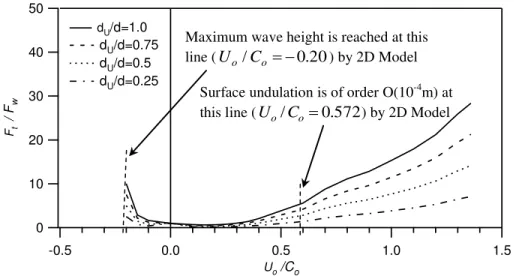
As an example, the established model has been applied for the computation of loads for a collinear or 2D case and for an oblique or 3D case. For both examples, it is assumed that a monochromatic current-free surface wave interacts with a normalized wave-free uniform current Uo/Co varying over the range of an opposite current to a range of following

currents. It is also assumed that the surface current is uniform and acting over a layer of fluid that extends from the free surface to a specified finite depth. The extent of this layered-current is defined by the ratio of the layered-current depth, dU to the mean water

depth, d and may be described by the ratio dU/d, see Fig. 8. The wave and current

all computations. Here the total loads and moments are calculated from the effects of the combined wave-current field as proposed above.

Table 7. Computational parameters

Parameters 2D Model 3D Model

Uo/Co (Maximum opposing) -0.20 -0.20 Uo/Co (Maximum following) 0.572 1.359 Ho/Lo 0.01 0.01 do/Lo 2.0 2.0 dU/d (Maximum) 1.0 1.0 dU/d (Minimum) 0.25 0.25

Wave incident direction 0 o 10o

Current incident direction 0 o 15o

Descriptions of maximum and minimum loads obtained by the above model for 2D collinear, non-oblique case are given in Fig. 9 and Fig. 10, respectively. In the 2D case we have found that the monochromatic wave that we have used in our computation, becomes

O(10-4m) (w.r.t. incident wave) when normalized current parameter reaches the value

Uo/Co = 0.572 for the case of a wave with a following current.

50 40 30 20 10 0 Ft / F w 1.5 1.0 0.5 0.0 -0.5 U_o /C_o d_U/d=1.0 d_U/d=0.75 d_U/d=0.5 d_U/d=0.25

Fig. 9 Normalized maximum exerted loads computed by the 2D Model for different layered currents.

For the case when wave and current are in opposite directions the maximum wave height is reached at Uo/Co = -0.2. Maximum wave height is reached due to wave blocking.

At this point wave steepness exceeds the allowable breaking value (~0.14) and the numerical model is stopped. These limits are shown in Fig. 9 and in Fig. 10 by a vertical dotted line. The analyses and comparisons of loads for 2D non-oblique case are again made at these two points, that is, when Uo/Co = 0.572 and Uo/Co = -0.20.

On the other hand when wave and current are in opposite directions the maximum and minimum loads obtained at Uo/Co = -0.20. Table 8 shows the results of the loads and

moments when the layered current is extended from the free surface to the bottom of the domain. The moment arm (M ) in this case isd 2.

Surface undulation is of order O(10-4m) at this line (Uo/Co0.572) by 2D Model

Maximum wave height is reached at this line (Uo/Co0.20) by 2D Model

50 40 30 20 10 0 -10 -20 Ft / F w 1.5 1.0 0.5 0.0 -0.5 U_o /C_o d_U/d=1.0 d_U/d=0.75 d_U/d=0.5 d_U/d=0.25

Fig. 10 Normalized minimum exerted loads computed by the 2D Model for different layered currents.

Table 8. Loads for 2D case: wave with following current Load Uo/Co Ft/Fw Mt/Mw

Maximum 0.572 5.614554 -5.62134 Minimum 0.572 5.614183 -5.62134 Loads for 2D case: wave with opposing current Maximum -0.20 10.02994 -10.012 Minimum -0.20 -10.3892 10.407

In the figures Mt stands for the total moment due to combined wave-current field or due

to wave-free current field. Mw describe the absolute moment due to the current-free wave

field.

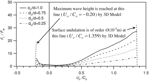
5.3.2 Load and moment computation by the 3D model for layered surface currents

For the oblique interaction cases the above mentioned wave and current conditions are used (as shown in Table 1) and in addition, it is assumed that the wave enters the computational domain at an oblique angle of 10o, while the current is at an angle of 15o with the positive direction of the x-axis. Figs. 11 and 12 demonstrate the comparison between the maximum and minimum loads and moments obtained by the above 3D model for different surface layered current depth. In the 3D oblique case, the analyses of loads and moments are also made at two points, at Uo/Co = 1.359 when surface undulation is of O(10-4m) due to a wave with a following current and at Uo/Co = -0.20 when the wave is in

opposite direction of the current shown by vertical dotted line in Fig. 11 and 12.

Surface undulation is of order O(10-4m) at this line (U_o/C_o0.572) by 2D Model Maximum wave height is reached at this line (U_o/C_o0.20) by 2D Model

50 40 30 20 10 0 Ft / F w 1.5 1.0 0.5 0.0 -0.5 U_o /C_o d_U/d=1.0 d_U/d=0.75 d_U/d=0.5 d_U/d=0.25

Fig. 11 Normalized maximum exerted loads computed by the 3D Model for different layered currents. 50 40 30 20 10 0 -10 -20 Ft / F w 1.5 1.0 0.5 0.0 -0.5 U o /Co dU/d=1.0 d_U/d=0.75 d_U/d=0.5 d_U/d=0.25

Fig. 12 Normalized minimum exerted loads computed by the 3D Model for different layered currents.

In the absence of wave(s) the model still compute the loading imparted by the wave-free current field shown in the figures after the vertical dotted line.

Table 9. Loads for 3D case: wave with following current Load Uo/Co Ft/Fw Mt/Mw

Maximum 1.359 26.28006 -27.4581 Minimum 1.359 23.85693 -27.4581 Loads for 3D case: wave with opposing current Maximum -0.20 6.21917 -6.29528 Minimum -0.20 -6.57534 6.65449

Surface undulation is of order O(10-4m) at this line (Uo/Co 1.359) by 3D Model

Maximum wave height is reached at this line (Uo/Co0.20) by 3D Model

Surface undulation is of order O(10-4m) at this line (U_o/C_o1.359) by 3D Model

Maximum wave height is reached at this line (Uo/Co0.20) by 3D Model

On the other hand, when wave and current are in opposite directions the maximum and minimum loads and moments are obtained at Uo/Co = -0.20. For the 3D oblique case we

have not proceeded after Uo/Co = 1.359 since wave height at this current becomes O(10

-4

m). Table 9 represents the maximum and minimum loads and moments for Uo/Co = 1.359

and Uo/Co = -0.20. In this case also, Table 9 shows the results of the loads and moments

when the layered current is extended from the free surface to the bottom of the domain. Again the moment arm (Ma) isd 2.

5.3.3 Moment computation by 2D model for layered surface currents

Figs. 13 and 14, respectively show the maximum and minimum moment for 2D flow fields computed by equation (63) for the cases when waves coexist with a surface current that is uniform and acting over a layer of fluid that extends from the free surface to a specified finite depth. The total moment due to combined wave and layered current field

t

M is normalized by the moment due to wave onlyM_w. The moment arms (M_a)for various wave and layered currents are computed by equation (63) shown in Table 10.

Table 10 Moment arms (Ma) to depth

o o C U M_a /d ) 0 . 1 / (d_U d d M_a / ) 75 . 0 / (d_U d d M_a / ) 50 . 0 / (dU d d M_a / ) 25 . 0 / (d_U d -0.2 0.496772 0.621 0.745158 0.869352 -0.15 0.498201 0.622 0.747301 0.871852 -0.1 0.499203 0.624 0.748804 0.873605 0 0.5 0.5 0.5 0.5 0.1 0.5 0.624 0.75 0.875 0.15 0.5 0.625 0.75 0.875 0.2 0.5 0.625 0.75 0.875 0.25 0.5 0.625 0.75 0.875 0.3 0.5 0.625 0.75 0.875 0.35 0.5 0.625 0.75 0.875 0.4 0.5 0.625 0.75 0.875 0.5 0.5 0.625 0.75 0.875 0.6 0.5 0.625 0.75 0.875 0.7 0.5 0.625 0.75 0.875 0.8 0.5 0.625 0.75 0.875 0.9 0.5 0.625 0.75 0.875 1 0.5 0.625 0.75 0.875 1.1 0.5 0.625 0.75 0.875 1.2 0.5 0.625 0.75 0.875 1.3 0.5 0.625 0.75 0.875 1.359 0.5 0.625 0.75 0.875

50 40 30 20 10 0 M t /M w 1.5 1.0 0.5 0.0 -0.5 U_o /C_o d_U/d=1.0 d_U/d=0.75 d_U/d=0.5 d_U/d=0.25

Fig. 13 Normalized maximum moments computed by the model in 2D flow

50 40 30 20 10 0 -10 -20 M t / M w 1.5 1.0 0.5 0.0 -0.5 U o /Co dU/d=1.0 d_U/d=0.75 d_U/d=0.5 d_U/d=0.25

Fig. 14 Normalized minimum moments computed by the model in 2D flow

5.3.4 Moment computation by 3D model for layered surface currents

Figs. 15 and 16 respectively show the maximum and minimum moment for 3D flow fields computed by equation (63) for the cases when waves coexist with a surface current that is uniform and acting over a layer of fluid that extends from the free surface to a specified finite depth. In the figures total moment due to combined wave-current field Mt is

normalized by the moment due to wave Mw.

Surface undulation is of order O(10-4m) at this line (U_o/C_o0.572) by 2D Model Maximum wave height is reached at this line (Uo/Co0.20) by 2D Model

Surface undulation is of order O(10-4m) at this line (Uo/Co0.572) by 2D Model

Maximum wave height is reached at this line (Uo/Co0.20) by 2D Model

50 40 30 20 10 0 M t /M w 1.5 1.0 0.5 0.0 -0.5 U_o /C_o d_U/d=1.0 d_U/d=0.75 d_U/d=0.5 d_U/d=0.25

Fig. 15 Normalized maximum moments computed by the model in 3D flow

50 40 30 20 10 0 -10 -20 M t / M w 1.5 1.0 0.5 0.0 -0.5 U o /Co dU/d=1.0 d_U/d=0.75 d_U/d=0.5 d_U/d=0.25

Fig. 16 Normalized minimum moments computed by the model in 3D flow

6. Conclusion

A 3D numerical model has been developed using three-dimensional expressions describing the characteristics of the combined wave-current field in terms of mass, momentum and energy flux conservation equations. The obtained model is then employed for the computation of the resulting combined wave-current field direction and kinematics and total loading on a slender vertical cylinder in 2D and in 3D flow field. Equations (31) to (36) produce the governing conservation equations when Equations (26), (28) and (30) are used to formulate the unknown quantities for the cases of wave, current and wave-current conditions. The obtained equations are used for the numerical computation of the combined field parameters. Maple software environment is used for the iterative solution of the nonlinear system of conservation equations and free-surface dispersion relation. In the computations Equations (48) is used [equations (53) or (58) can also be used] to find the direction of the combined wave-current field while Equations (47), (52) and (57)

Surface undulation is of order O(10-4m) at this line (U_o/C_o 1.359) by 3D Model Maximum wave height is reached at this line (Uo/Co0.20) by 3D Model

Surface undulation is of order O(10-4m) at this line (U_o/C_o 1.359) by 3D Model Maximum wave height is reached at this line (Uo/Co 0.20) by 3D Model

together with equation (43) are utilized for the computation of the after-interaction surface disturbance height H, its length L, mean water depth d, current like parameter U, and the variation of the direction of the combined wave-current field. Examples for collinear 2D non-oblique waves and currents and an oblique 3D case are shown. The present 2D and 3D combined wave-current models are compared with S2D and S3D superposition models. The comparisons show that superposition models are less effect for the computations of loads especially when waves and currents are in opposite direction. Four different categories of current field considering its extent from the free surface to a certain water depth are also considered for load and moment computation by the numerical 2D and 3D numerical models. It is observed as expected that load on the vertical cylinder is directly proportional to dU/d ratios, i.e. when dU/d is greater the loading on the cylinder is also

larger. Similar phenomenon is observed for moments of different current depths from the free surface. It is necessary to mention here that for the case of wave with following current, even when waves disappear due to strong current, the present model is still applicable for the computation of loading due to current only. In another words this 3D (also 2D) model is capable to compute loads in the presence of current only cases.

References

Baddour, R.E. and Song, S.W., 1990a. On the interaction between waves and currents. Ocean Engineering, 17 (1/2), 1-21.

Baddour, R.E and Song, S.W., 1990b. Interaction of higher-order water waves with uniform currents. Ocean Engineering, 17 (6), 551-568.

Chakrabarti, S., 2005. Handbook of offshore engineering. Elsevier, 1, 661.

Chakrabarti, S. K., 1987. Hydrodynamics of offshore structures. Computational Mechanics Publication, Springer-Verlag, 1-440.

Dean, R.G. and Dalrymple, R.A., 1992. Water wave mechanics for engineers and scientists. Prentice-Hall Inc, Englewood Cliffs, NJ, 66-69.

Hedges, T.S. and Lee B.W., 1991. The equivalent uniform in wave-current computations. Coastal Engineering, 16, 301-311.

Iwagaki, Y., Asano, T. and Nagai, F., 1983. Hydrodynamic forces on a circular cylinder placed in the wave-current co-existing fields, Memoirs of the Faculty of Engineering,

Kyoto University, Japan, XLV(1), 11-23.

Kemp, P. H. and Simons R. R., 1982. The interaction between waves and a turbulent current: waves propagating with the current. Journal of Fluid Mechanics, 116, 227-250. Kemp, P. H. and Simons R. R., 1983. The interaction of waves and a turbulent current: waves propagating against the current. Journal of Fluid Mechanics, 130, 73-89.

Longuet-Higgins, M.S. and Stewart, R.W., 1960. Changes in the form of short gravity waves on long waves and tidal currents. Journal of Fluid Mechanics, 8, 565-583.

Longuet-Higgins, M.S. and Stewart, R.W., 1961. The changes in amplitude of short gravity waves on steady non-uniform currents. Journal of Fluid Mechanics, 10, 529-549. Maple-12, Language reference manual, Waterloo Maple Publishing, Springer-Verlag, Heidelberg, NY, 2008.

Morison, J. R., O’Brien, M. P., Johnson, J. W. and Schaaf, S. A.. 1950. The forces exerted by surface waves on piles. Petroleum Trans., AIME, Vol. 189, 149-157.

Sarpkaya, T. and Isaacson, M.. 1981. Mechanics of wave forces on offshore structures.

Van Nostrand Reinhold Company Inc, 1-651.

Whitham, G.B., 1962. Mass, momentum and energy flux in water waves. Journal of Fluid Mechanics, 12, 135-147.

Thomas, G. P., 1981. Wave-current interactions: an experimental and numerical study. Part 1. Linear waves. J. Fluid Mech., 110, 457-474.

Zaman, M. H., Togashi, H. and Baddour, E., 2010. Interaction of waves with non-colinear currents. Ocean Engineering, 38 (4), 541-549.

Zaman, M. H., Togashi, H. and Baddour, E., 2008. Deformation of monochromatic water waves propagating over a submerged obstacle in the presence of uniform current. Ocean Engineering, 35 (8-9), 823-833.

Zaman, M. H. and Baddour, R. E., 2006. Wave-current loading on a vertical slender cylinder by two different numerical models, 25th Int. Conf. on offshore Mech. and Arctic Eng. (OMAE-2006), ASME, Hamburg, Germany, 8 pages, on CD-ROM.

Zaman, M. H. and Baddour, R. E., 2005. Combined loading of a wave and surface current on a fixed vertical slender cylinder. 24th Int. Conference on offshore Mechanics and Arctic Engneering, OMAE-2005, ASME, Halkidiki, Greece, 8 pages, on CD-ROM.

Zaman, M. H. and Baddour, R. E., 2004. Loading on a fixed vertical slender cylinder in an oblique wave-current field, 23rd Int. Conf. on offshore Mech. and Arctic Eng. (OMAE-2004), ASME, Vancouver, 9 pages, on CD-ROM.

Zaman, M. H. and Baddour, R. E., 2002. Waves and currents interacting in a 3D field. International Conference on Ship and Ocean Technology (SHOT-2002), IIT-Kharagpur, India, (on CD-ROM)

Zaman, M. H. and Togashi, H., 1996. Experimental study on interaction among waves, currents and bottom topography. Proceedings Civil Engineering in the Ocean, JSCE, 12, 49-54.