Publisher’s version / Version de l'éditeur:
HVAC and R Research, 20, 1, pp. 92-112, 2014-01-08
READ THESE TERMS AND CONDITIONS CAREFULLY BEFORE USING THIS WEBSITE.
https://nrc-publications.canada.ca/eng/copyright
Vous avez des questions? Nous pouvons vous aider. Pour communiquer directement avec un auteur, consultez la première page de la revue dans laquelle son article a été publié afin de trouver ses coordonnées. Si vous n’arrivez pas à les repérer, communiquez avec nous à PublicationsArchive-ArchivesPublications@nrc-cnrc.gc.ca.
Questions? Contact the NRC Publications Archive team at
PublicationsArchive-ArchivesPublications@nrc-cnrc.gc.ca. If you wish to email the authors directly, please see the first page of the publication for their contact information.
NRC Publications Archive
Archives des publications du CNRC
This publication could be one of several versions: author’s original, accepted manuscript or the publisher’s version. / La version de cette publication peut être l’une des suivantes : la version prépublication de l’auteur, la version acceptée du manuscrit ou la version de l’éditeur.
For the publisher’s version, please access the DOI link below./ Pour consulter la version de l’éditeur, utilisez le lien DOI ci-dessous.
https://doi.org/10.1080/10789669.2013.834779
Access and use of this website and the material on it are subject to the Terms and Conditions set forth at
Practical correlation for thermal resistance of low-sloped enclosed
airspaces with downward heat flow for building applications
Saber, H.H.
https://publications-cnrc.canada.ca/fra/droits
L’accès à ce site Web et l’utilisation de son contenu sont assujettis aux conditions présentées dans le site LISEZ CES CONDITIONS ATTENTIVEMENT AVANT D’UTILISER CE SITE WEB.
NRC Publications Record / Notice d'Archives des publications de CNRC:
https://nrc-publications.canada.ca/eng/view/object/?id=9b8e8ebb-c39d-40eb-a58d-b48961d18639 https://publications-cnrc.canada.ca/fra/voir/objet/?id=9b8e8ebb-c39d-40eb-a58d-b48961d18639Practical correlation for thermal resistance of low-sloped
enclosed airspaces with downward heat flow for building
applications
Hamed H. Saber
NRC-Construction, National Research Council of Canada, 1200 Montreal Road, Ottawa
Ontario, K1A 0R6, Canada
Abstract
The 2009 ASHRAE Handbook of Fundamentals (Chapter 26) provided a table that contains the thermal resistances (R-values) of vertical, horizontal, and high-sloped (45o) enclosed airspaces. This table is extensively
used by modellers, architects and building designers in the design for the R-values of building enclosures. The effect of the airspace aspect ratio and the inclination angle () of 30oon the R-values are not accounted for in the
ASHRAE table. However, previous studies showed that the aspect ratio of the airspace can affect its R-value. In this paper, the previous studies that focused on determining the R-values for vertical, horizontal, and high-sloped enclosed airspaces are extended to investigate the effect of the aspect ratio on the R-values of low-sloped (= 30o)
enclosed airspaces under downward heat flow for different airspace thicknesses and having a wide range of values for the effective emittance, mean temperature, and temperature differences across the airspaces. Thereafter, practical correlation is developed for determining the R-values of low-sloped enclosed airspaces for future use by modellers, architects and building designers.
Keywords: Reflective insulation, low emissivity material, thermal modelling, R-value correlation, airflow in
enclosed airspace, and heat transfer by convection, conduction & radiation.
Introduction
In regions with harsh climatic conditions, a substantial share of energy is used for heating and cooling the buildings (Al-Homoud 2005). Energy consumption of the building sector is high and although the situation differs from country to country, buildings are responsible for about 30-40% of the total energy demand (Vrachopoulos et al.
2012). In Europe, however, buildings are responsible for 40-50% of energy use and the largest share of energy in buildings is used for heating (European Commission 2010). The design of building enclosures with the intent of achieving energy savings can necessarily help reduce building operating loads and thus the demand for energy over time (Saber et al. 2011a, 2012a). Thermal insulations are major contributors and obviously a practical and logical first step towards achieving energy efficiency especially in buildings located in sites with harsh climatic conditions. This can evidently be achieved by increasing the effective thermal resistance (R-value) of the building envelope.
Reflective Insulation (RI) products are typically being used in conjunction with mass insulation products, such as glass fibre, expanded polystyrene foam (EPS), and other similar insulation products. The RI products were introduced onto the building market as a promising thermal insulation material. According to the installation guidelines of the Reflective Insulation Manufacturers Association International (RIMA-I 2002), RI products have at least one reflective surface facing an airspace. The RI products can be installed in wall cavities, between ceiling and floor joists, and in metallic buildings that cannot readily accommodate loose-fill or batt-type insulations. Also, RI products can be used as part of a roofing system either below the decking between rafters, within small air gaps between decking and roofing, and in air gaps created, for example, by paneling interior masonry walls (Yarbrough 1983).
A comprehensive review about the use of reflective materials to reduce heat transfer by radiation across enclosed airspaces was conducted by Gross and Miller (1995). Fricker and Yarbrough (2011) conducted literature review on four computational methods for evaluating the R-values of enclosed reflective airspaces. Those four methods involved an assumption of one-dimensional heat transfer between large parallel surfaces (infinite parallel planes). In an actual building enclosure, however, there are surfaces connecting the parallel planes (framing). These surfaces absorb, emit and reflect radiation. Glicksman (1991) has shown that the heat transfer process that included radiation interaction between the parallel surfaces and the framing resulted in a decrease in the overall performance (i.e. lower R-values).
It is important to determine the effective R-values of the airspaces of different dimensions, effective emittances, inclination angles, directions of heat flow, mean airspace temperatures, and temperature differences across the airspaces. Many studies were conducted to determine the R-values of RI products, and wall and roofing systems incorporating RI products (Yarbrough 1983, Fairey 1985, Han et al. 1986, Desjarlais and Tye 1990, Desjarlais and Yarbrough 1991, Medina 2000, Al-Homoud 2005, European Commission 2010, Saber and Swinton
2010, Craven and Garber-Slaght 2011, Saber et al. 2011b,c, Vrachopoulos et al. 2012, D’Orazio et al. 2012, Saber and Maref 2012, Saber et al. 2012a,b,c, Escudero et al. 2013, Tenpierik and Hasselaar 2013, Saber 2013a,b,c,d,e). Also, there are many claims indicating that RI products can have high thermal resistance. Debate is still ongoing into whether these claims are correct (Tenpierik and Hasselaar 2013). However, some in situ measurements, and hot box and hot plate measurements performed in laboratories resulted in lower R-values. For example, Saber (2012a) and Saber et al. (2012b) showed that a heat flow meter in accordance with standard ASTM C-518 (ASTM 2003) underestimates the effective R-value of RI products that include radiation shields in combination with horizontal enclosed airspaces. The main reason lies in non-uniform convective flows in these airspaces. As such, Tenpierik and Hasselaar (2013) conducted an extensive literature review to identify the causes for the different results among different research organizations. D’Orazio et al. (2012) conducted field study under hot climatic conditions to investigate the thermal performance of an insulated roof with RI product. The results of that study showed that the benefits of RI product are quite limited when using the insulation level imposed by actual laws, which consider insulation as the main strategy for energy saving in temperate and hot climates.
This paper focuses on determining the R-values of enclosed airspaces under different operation conditions. Note that the term “enclosed” is critical since the major distinction between RIs and Radiant Barriers (RBs) is the airspace condition, where the RB system is defined as a building construction that consists of a low emittance surface bounded by an “open” airspace (Fairey 1985, Desjarlais and Tye 1990, Medina 2000, Al-Homoud 2005). The parameters that affect the R-value of an enclosed airspace are: the physical properties of the air filling the space, the temperature and emissivity of all surfaces of the airspace, temperature differences across the airspace, the dimensions of the airspace, the direction of heat flow through the airspace, and the orientation of the airspace. The R-values of enclosed airspaces were calculated by many investigators (e.g. see Robinson and Powlitch 1954, Robinson et al., 1954, 1956) for various orientations of airspaces and reflective boundaries by using heat transfer coefficient data that was published by Robinson et al. (1954, 1956). The heat transfer coefficient data were obtained from measurements of panels of different thicknesses using the test method described in the ASTM C236-53 (ASTM 1953). In those studies, the steady-state heat transmission rates were corrected for heat transfer occurring along parallel paths between hot and cold boundaries. Thereafter, the convective heat transfer coefficients were obtained from the data by subtracting a calculated radiative heat transfer rate from the total corrected heat transfer rate; and the radiative heat transfer was calculated using an emissivity of 0.028 for the aluminum surfaces.
The 2009 ASHRAE Handbook of Fundamentals, Chapter 26 (ASHRAE 2009) provides a table that contains the R-values for enclosed airspaces of three inclination angles () of 0o, 45oand 90o, which were determined on the basis of the heat transfer data reported by Robinson et al. (1954, 1956). These R-values are being extensively used by modellers, architects and building designers to determine the values of building enclosures. The ASHRAE values were obtained by combining the convective and radiative components of heat transfer from which the total R-value for an enclosed airspace was provided for airspaces of different thickness ( = 13 mm (0.5 in), 20 mm (0.75 in), 40 mm (1.5 in), and 90 mm (3.5 in)), mean temperature (Tavg= 32.2oC (90oF), 10.0oC (50oF), -17.8oC (0oF) and -45.6oC (-50oF)), temperature difference across the airspace (T = 5.6oC (10oF), 11.1oC (20oF) and 16.7oC (30oF)), effective emittance (eff= 0.03, 0.05, 0.2, 0.5 and 0.82), and direction of heat flow through the airspace. Note that the effective emittance (εeff) of an enclosed airspace is given as (ASHRAE 2009):
, 1 / 1 / 1 / 1 eff 1 2 (1)
where 1and2 are the emissivity of the hot and cold surfaces (see Figure 1). It is worth mentioning that the R-values of low-sloped enclosed airspaces (the focus of this study) are not available in the ASHRAE table. Furthermore, the effect of the aspect ratio (length/thickness) of the enclosed airspace on the R-values is not accounted for in the ASHRAE table (ASHRAE 2009). In recent studies (Saber 2013b,c,d,e), the NRC’s hygrothermal model, called hygIRC-C, was used to predict the R-values of vertical, horizontal, and high-sloped (45o) enclosed airspaces for a wide range of airspace different thickness, aspect ratio, mean temperature, temperature differential, effective emittance, and direction of heat flow. In this study, this model was used to investigate the thermal performance of low-sloped (30o) enclosed airspaces with downward heat flow and subjected to different operating conditions. The model description and benchmarking are discussed next.
Model description and boundary conditions
The numerical model that was used in study solves simultaneously the 2D and 3D moisture transport equation, energy equation, surface-to-surface radiation equation (e.g. surface-to-surface radiation in enclosed airspace such as shown in Figure 1) and air transport equation in the various material layers. The air transport equation is the Navier-Stokes equation for the airspace (e.g. air cavity), and Darcy equation (Darcy Number, DN <10-6) and Brinkman equation (DN > 10-6) for the porous material layers (see Saber et al. 2010a,b, 2011a,b,c, and 2012a,b,c,d for more
details) In this study, no moisture transport was accounted for. As shown in Figure 1, the boundary conditions that are needed to solve the energy equation are: (a) adiabatic condition (i.e. no heat transport) on the two sides of the enclosed airspace, and (b) temperature boundary conditions on the top surface (high temperature, TH) and the bottom surface (low temperature, TC) for the case of downward heat flow. Also the boundary conditions that are needed to solve the Navier-Stokes equation for the air cavity are no-slip condition on all surfaces of the enclosed airspace.
Model Benchmarking
In this study, the numerical simulation model described above was used to determine the effective R-values of low-sloped enclosed airspaces of = 30o. The airspaces were subjected to downward heat flow for the same parameters listed in ASHRAE table (ASHRAE 2009). This model had been previously benchmarked in a number of building applications (e.g. see Air Ins 2009, Saber et al. 2011b, 2012b, Saber 2012a). For the applications that are similar to this study, the numerical model was benchmarked against the thermal performance data for a full-scale wall assembly featuring a reflective insulation product. The data was obtained using a Guarded Hot Box (GHB) in accordance with ASTM C-1363 test method (ASTM 2006). Results showed that the R-value predicted by the model for this wall system was in good agreement with the measured R-value (within 1.2%) (Air Ins 2009, Saber et al. 2011b). Furthermore, the numerical model was benchmarked against a number of tests that were conducted at the Cold Climate Housing Research Center (CCHRC) (Craven and Garber-Slaght 2011) and the National Research Council of Canada (NRC) (Saber 2012a, Saber et al. 2012b). These tests were conducted using heat flow meters in accordance with the ASTM C-518 test method (ASTM 2003) to examine the thermal performance of different types of reflective insulation assemblies. The results showed that the heat fluxes predicted by the model were in good agreements with the measured heat fluxes (within 1.0%). Thereafter, the model was used to investigate the contribution of reflective insulations to the R-value for specimens having three inclination angles ( = 0o, 45oand 90o), different directions of heat flow through the specimens, and a wide range of foil emissivity (Saber 2012a).
In previous studies, the model was used to determine the R-values of vertical enclosed airspaces ( = 90o) (Saber 2013b), horizontal enclosed airspaces ( = 0o) with upward heat flow (Saber 2013c) and downward heat flow (Saber 2013e), and high-sloped enclosed airspaces ( = 45o) with downward heat flow (Saber 2013d). In those studies, the predicted R-values were compared with the ASHRAE R-values (ASHRAE 2009) for enclosed airspaces of different thicknesses and different operating conditions. The dependence of the R-value on the aspect ratio (A )
of the enclosed airspace was also investigated in those studies. The results showed that depending on the thickness of the enclosed airspace and the operating conditions, the aspect ratio can have a significant effect on the R-value. Furthermore, practical correlations were developed for determining the R-values of enclosed airspaces of = 0o, 45o and 90oof different thicknesses (), and for a wide range of values for various parameters (A
R, T, Tavg, and eff). The results showed that the calculated R-values using those correlations were in good agreements with those obtained using the model (within ±3% to ±5%) (Saber 2013b,c,d,e). A full description of the present model and more details about model benchmarking are available in previous publications (Elmahdy et al. 2009, Saber and Swinton 2010, Saber et al. 2010a,b, 2011a,b,c, 2012a,b,d, Saber and Maref 2012, Saber 2012a,c, 2013a).
Objectives
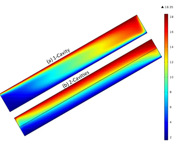
As indicated earlier, practical correlations were developed in previous studies for determining the R-values of enclosed airspaces of = 0o, 45oand 90o(Saber 2013b,c,d,e). In this study, the thermal performance of low-sloped enclosed airspaces ( = 30o) with downward heat flow are explored so as to cover a wide range of inclination angles for different building applications. To ensure that the differences in the R-values for low-sloped ( = 30o) enclosed airspaces, and that for = 0o, 45o & 90o are large enough and worth of investigation, preliminary numerical simulations were conducted for enclosed airspaces of different thickness ( = 13 mm (0.5 in), 20 mm (0.75 in), 40 mm (1.5 in) and 90 mm (3.5 in)) at = 30o, T
avg= 10oC (50oF), T = 16.7oC (30oF), and H = 305 mm (12 in). The obtained R-values were compared in Figure 2 with that for enclosed airspaces of different orientations (vertical: = 90o, Saber 2013b, horizontal: = 0o, Saber 2013e, and = 45o, Saber 2013d). The enclosed airspaces of = 0o, 30o and 45owere subjected to downward heat flow. As shown in Figure 2, for a given and
eff, the R-values increases by decreasing the inclination angle and reached its highest for the case of = 0o (Saber 2013e). Because the contribution of heat transfer due to natural convection in enclosed airspaces of large thickness is higher than that for enclosed airspaces of small thickness, Figure 2 shows that the inclination angles have a significant effect on the R-values of enclosed airspaces of large thickness compared to that for enclosed airspaces of small thickness. For example, at eff= 0.05, by considering the vertical enclosed airspace as a reference (i.e. = 90o), decreasing the inclination angle from 90o(Saber 2013b) to 45o(Saber 2013d), 30o, and 0o(Saber 2013e) resulted in an increase of the R-value, respectively, by: (a) 5%, 8% and 12% for = 13 mm (0.5 in) (Figure 2a), (b) 11%, 22% and 54% for
= 20 mm (0.75 in) (Figure 2b), (c) 14%, 28% and 147% for = 40 mm (1.5 in) (Figure 2c), and (d) 21%, 46% and 208% for = 90 mm (3.5 in) (Figure 2d). Furthermore, at eff= 0.05, decreasing the inclination angle from 45oto 30oresulted in an increase of the R-value by 3%, 11%, 12% and 21% for = 13 mm (0.5 in), 20 mm (0.75 in), 40 mm (1.5 in), and 90 mm (3.5 in), respectively.
The results presented above and shown in Figure 2 indicate that it is worth to investigate the thermal performance of low-sloped enclosed airspaces. As such, the previous studies (Saber 2013b,c,d,e) in which numerical simulations were conducted to determine the R-values of enclosed airspaces of = 0o, 45oand 90oare extended in order to investigate the thermal performance of low-sloped enclosed airspaces of = 30oand subjected to a downward heat flow with different Tavgand T. The objectives of this study are to:
Investigate the potential increase in the R-value of an enclosed airspace when a thin sheet having an emissivity ranging between 0.0 to 0.9 is installed in the middle of a 30osloped enclosed airspace.
Investigate the effect of the aspect ratio (AR) on the R-value of low-sloped enclosed airspaces of different thicknesses ( = 13 mm (0.5 in), 20 mm (0.75 in), 40 mm (1.5 in) and 90 mm (3.5 in)) for a wide range of effective emittance values (eff= 0 – 0.82).
Develop practical correlation for the R-values of enclosed airspaces covering a wide range of values for AR, Tavg, T, and efffor subsequent use in currently available energy simulation models (e.g. ESP-r, Energy Plus, DOE).
Results and discussions
This section presents the results of the numerical simulations that were conducted in order to determine the effective R-values of low-sloped enclosed airspaces ( = 30o) with a downward heat flow for the same parameters listed in ASHRAE (ASHRAE 2009): (a) thickness ( = 13 mm (0.5 in), 20 mm (0.75 in), 40 mm (1.5 in) and 90 mm (3.5 in)), (b) mean temperature (Tavg = 32.2oC (90oF), 10.0oC (50oF), -17.8oC (0oF) and -45.6oC (-50oF)), (c) temperature difference across the airspace (T = 5.6 (10oF), 11.1oC (20oF) and 16.7oC (30oF)), and (d) effective emittance (eff= 0 – 0.82). For a given value of , numerical simulations were conducted for a wide range of airspace length (H) in order to: (i) quantify the effect of the airspace aspect ratio (AR= H/) on the R-values of the airspace, and (ii) permit the development of practical correlation for determining R-values that cover most expected
building applications having low-sloped enclosed airspaces. Examples of these applications include planar sloped skylights, and Furred-Airspace Assemblies (FAA) attached to thermal insulation (bonded by Low Emissivity Material, LEM) in sloped roofing systems having furring of different center-to-center spacings.
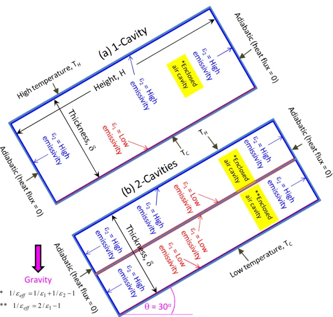
Figure 1a shows a schematic of a low-sloped enclosed airspace of inclination angle () of 30oin which only one surface of the airspace has a low emissivity (1), and all other surfaces have a high emissivity (2). Most construction materials have an emissivity of 0.9 (ASHRAE 2009). In this study, the numerical simulations were conducted for different values of 1(ranging from 0 – 0.9) and 2was taken equal to 0.9. According to Eq. (1), a wide range of values of the effective emittance, eff(ranging from 0 – 0.82) were considered. The value of effof 0.82 represents the case when all surfaces of the enclosed airspace have an emissivity of 0.9 (i.e. no LEM installed on the surfaces of the enclosed airspace).
For an enclosed airspace of H = 305 mm (12 in), numerical simulations were also conducted in order to investigate the potential increase in the R-values of the enclosed airspace when a thin sheet (0.1 mm thick) is placed in the middle of the airspace and whose surfaces having a low emissivity (1) (see Figure 1b). The thin sheet divides the enclosed airspace into two cavities of equal thickness. It was assumed that no cross airflow occurs between the two cavities. The numerical simulations were conducted for a wide range of values for , 1, Tavg, and T. In this paper, the simulation case for which there is no thin sheet inside the airspace is referred to as “1-Cavity” (Figure 1a), whereas “2-Cavities” refers to the case with a thin sheet in the middle of the airspace (Figure 1b).
Comparisons between the thermal performance of “1-cavity” and “2-cavities”
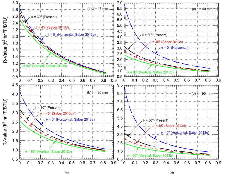
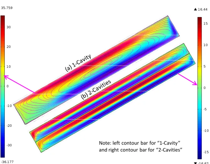
As an example for Tavg= 10oC (50oF), T = 16.7oC (30oF) (TH= 18.35oC (65oF) and TC= 1.65oC (35oF)), 1= 0.05, and 2= 0.9, Figure 3 and Figure 5 show the temperature contours inside the enclosed airspace (H = 305 mm (12 in)) for values of of 90 mm (3.5 in) and 40 mm (1.5 in), respectively. The corresponding streamlines and the contours of the vertical air velocities are shown in Figure 4 for = 90 mm (3.5 in), and in Figure 6 for = 40 mm (1.5 in). Owing to the temperature differential across the enclosed airspace, a buoyancy-driven flow is developed within the airspace. A cellular airflow is developed within each enclosed airspace for the cases of “1-Cavity” and “2-Cavities”. Figure 4 and Figure 6 for the vertical air velocities show that these air velocities for the “1-Cavity” simulation case are significantly higher than that for the “2-Cavities” case. The maximum values of the upward (+ve) and downward (-ve) vertical velocities (uy), and the right (+ve) and left (-ve) horizontal velocities are
compared in Table 1 for “1-Cavity” and “2-Cavities” simulation cases at airspace thicknesses of 40 mm (1.5 in) and 90 mm (3.5 in). As shown in this table, the maximum air velocities in the airspace are greater for the “1-Cavity” case as compared to the “2-Cavities” case by a factor of ~1.4 – 1.7 and ~2.2 at = 90 mm (3.5 in) and 40 mm (1.5 in), respectively.
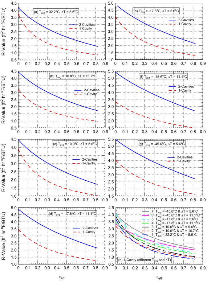
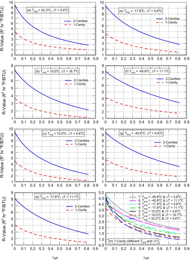
The higher air velocities for the case of “1-Cavity” resulted in a stronger convection current with one convection loop as compared to the “2-Cavities” case for which there was one convection loop in each cavity. Consequently, the rate of heat transfer by convection for the “1-Cavity” case is greater than that of the “2-Cavities” case resulting in higher thermal conductance (i.e. lower thermal resistance) in the “1-Cavity” as compared to the “2-Cavities” case. For enclosed airspaces of different thicknesses ( = 13 mm (0.5 in), 20 mm (0.75 in), 40 mm (1.5 in) and 90 mm (3.5 in)) at different eff, Tavgand T, comparisons between the R-values for the cases of “1-Cavity” and “2-Cavities” are provided in Figure 7 ( = 13 mm (0.5 in)), Figure 8 ( = 20 mm (0.75 in)), Figure 9 ( = 40 mm (1.5 in)) and Figure 10 ( = 90 mm (3.5 in)). For a given effective emittance, eff, these figures show that the R-values for the “2-Cavities” simulation case are higher than that of the “1-Cavity” case.
A practical example for creating “2-Cavity” solution is to install a thin sheet with low emissivity at the middle of the enclosed airspace. For the applications of planar skylights, windows and curtain wall systems, the thin sheet should be transparent that can be coated with a transparent material of low emissivity. However, for the applications of wall and roofing systems with enclosed airspaces, the thin sheet could be opaque (e.g. aluminum foil). The benefits of installing a thin sheet are: (a) reducing heat transfer by convection (see Table 1), and (b) reducing heat transfer by radiation due to low effective emittance (see Eq. (1)). These benefits result in higher R-value for the “2-Cavity” case compared to the “1-“2-Cavity” case (see Table 2). At eff= 0.03 and 0.82, Table 2 shows the percentage increase in the R-value due to the incorporation of a thin sheet in the middle of the enclosed airspace (see Figure 1b) and having an emissivity = 1on both sides of the thin sheet. Due to the incorporation of a thin sheet, this table shows that the percentage increase in the R-value increases as increases from 13 mm (0.5 in) to 20 mm (0.75 in) and 40 mm (1.5 in). This percentage increase in the R-value was approximately the same by further increasing from 40 mm (1.5 in) to 90 mm (3.5 in). For example, depending on the values of Tavg and T, the percentage increase in the R-value at eff= 0.03 changes from: (a) 8% to 15% for = 13 mm (0.5 in), (b) 20% to 65% for = 20 mm (0.75 in), (c) 98% to 124% for = 40 mm (1.5 in), and (d) 97% to 117% for = 90 mm (3.5 in) (Table 2).
Similarly, at eff= 0.82, the percentage increase in the R-value changes from: (a) 44% to 58% for = 13 mm (0.5 in), (b) 65% to 80% for = 20 mm (0.75 in), (c) 93% to 106% for = 40 mm (1.5 in), and (d) 89% to 92% for = 90 mm (3.5 in) (Table 2).
In summary, the R-value could be doubled due to installing a thin sheet in the middle of low-sloped enclosed airspaces ( = 30o) with downward heat flow. Also, it was shown in previous studies that the R-value could be doubled due to: (a) installing a thin sheet in the middle of high-sloped enclosed airspaces ( = 45o) with downward heat flow (Saber 2013d), (b) installing a thin sheet vertically in the middle of the vertical enclosed airspace ( = 90o) (Saber 2013b), and (c) installing a thin sheet horizontally in the middle of horizontal enclosed airspace ( = 0o) with downward heat flow (Saber 2013e). However, the R-value could be tripled if a thin sheet is installed horizontally in the middle of the horizontal enclosed airspace ( = 0o) with an upward heat flow condition (Saber 2013c). These results are important for future applications when a thin reflecting foil is placed in the middle of the enclosed airspace of planar skylights, windows, curtain wall systems, and Furred-Airspace Assemblies (FAA) attached to thermal insulation in wall and roofing systems so as to enhance the energy performance of these systems.
Dependence of the R-value on the aspect ratio
In previous studies, the dependence of the R-value on the aspect ratio, AR(AR= length (H)/thickness ()) of the vertical enclosed airspaces ( = 90o) (Saber 2013b), horizontal airspaces ( = 0o) with upward heat flow (Saber 2013c) and downward heat flow (Saber 2013e), and high-sloped airspaces ( = 45o) (Saber 2013d) were investigated. Depending on the thickness of the airspace and the operating conditions, the results of those studies showed that the aspect ratio can have a significant effect on the R-value. In this study for low-sloped enclosed airspaces ( = 30o) of different thickness ( = 13 mm (0.5 in), 20 mm (0.75 in), 40 mm (1.5 in) and 90 mm (3.5 in)) and subjected to downward heat flow, numerical simulations were conducted at Tavg= 32.2 (90oF), 10.0oC (50oF), -17.8oC (0oF) and -45.6oC (-50oF), T = 5.6oC (10oF), 11.1oC (20oF) and 16.7oC (30oF), and
eff= 0 – 0.82 in order to investigate the effect of the aspect ratio on the R-values. For a given airspace thickness, the numerical simulations were conducted for different lengths (H) ranging from 203 mm (8 in) to 2,438 mm (96 in). The obtained R-values are provided in Figure 11a-g ( = 13 mm (0.5 in)), Figure 12a-g ( = 20 mm (0.75 in)), Figure 13a-g ( = 40 mm (1.5 in)), and Figure 14a-g ( = 90 mm (3.5 in)).
Figure 11 through Figure 14 show that the R-value of an enclosed airspace of longer length is greater than that of an enclosed airspace of shorter length. Furthermore, for a given value of, these figures show that the amount of increase in the R-value due to increasing the aspect ratio depends on the values of Tavg, T and eff. For example, at Tavg= 10.0oC (50oF), T = 16.7oC (30oF) and eff= 0.03 for an enclosed airspace having a thickness of 13 mm (0.5 in), Figure 11b shows that increasing H from 203 mm (8 in) (AR= 16) to 2,438 mm (96 in) (AR= 188) resulted in an increase in the R-value by 10%. At these operating conditions (Tavg, T, and eff) for an enclosed airspace having a thickness of = 20 mm (0.75 in), an increase of H from 203 mm (8 in) (AR= 10) to 2,438 mm (96 in) (AR= 122) resulted in an increase of R-value by 44% (Figure 12b). Likewise as shown in Figure 13b for enclosed airspace of = 40 mm (1.5 in), an increase of H from 203 mm (8 in) (AR= 5) to 2,438 mm (96 in) (AR= 61) resulted in an increase of R-value by 52%. Finally, as provided in Figure 14b for enclosed airspace of = 90 mm (3.5 in), an increase of H from 203.2 mm (8 in) (AR= 2) to 2,438 mm (96 in) (AR= 27) resulted in an increase of R-value by 34%.
In summary, it is observed that the aspect ratio has a significant effect on the R-values of low-sloped enclosed airspace and subjected to downward heat flow condition. This observation is in agreement with the results from previous studies for vertical, horizontal, and high-sloped enclosed airspaces (Saber 2013b,c,d,e).
Practical correlation for the R-values
The results of the R-values that were presented in the previous section for low-sloped enclosed airspaces ( = 30o) of = 13 mm (0.5 in), 20 mm (0.75 in), 40 mm (1.5 in), and 90 mm (3.5 in), and as provided in Figure 11h through Figure 14h were used to develop practical correlation for the R-values. A correlation was developed for each value of to obtain the R-value in (ft2hroF/BTU) as a function of all parameters (i.e. T
avg, T, ARand eff). This correlation is given in the following form:
i eff i i c a avg R i i R i c a avg eff c a avg R avg c T a A T T a T T g A A T T b R value R
4 1 4 1 0 1 1 1 2 2 2 3 3 ) ( (2)In this correlation, Rc(Tavg) is the R-value in (ft2hroF/BTU) of the enclosed airspace due to heat transfer by conduction only, which is given as (Saber 2013b,c,d,e):
), ( / ) ( avg avg c T T R
(3) where, 15 -4 11 -3 8 -2 4 -1 0 4 0 10 1 -7.4386433 , 10 4.11702505 , 10 6 -7.9025285 , 10 1.15480022 3562, -0.0022758 , ) (
f f f f f T f T avgi i i avg (4)Note that
(Tavg) in Eq. (4) is the average thermal conductivity of air in (W/mK), which is evaluated at the mean temperature of the airspace, avgT in (K). It is important to point out that the calculated value of Rc(Tavg) from Eq. (3) and (4) must be converted to (ft2hroF/BTU) in order to be used in Eq. (2).In Eq. (2), the units of Tavg and T must be in (K). The other coefficients in Eq. (2) , , , , , ,
(a0 a b1 b2 b3 b4 1,2,,a1,a2,a3,c1,c2,c3,g1,g2,g3,andg4) are listed in Table 3. In order to develop an accurate correlation, these coefficients were obtained for two ranges of the effective emittance (eff< 0.2 and eff 0.2).
Close examinations for the correlation given by Eq. (2) reveal that the first term on the RHS represents the R-value due to heat transfer by conduction only. The second term on the RHS of this equation represents the reduction in the R-value due to heat transfer by convection only. Whereas the last two terms on the RHS of this equation represent the reduction in the R-value due to heat transfer by radiation only at different values of effective emittance (eff).
For a given thickness of low-sloped enclosed airspace ( = 30o) with a downward heat flow condition, the predicted R-values obtained using the numerical simulation model and shown in Figure 11h through Figure 14h were compared with those obtained using the correlation given in Eq. (2). These comparisons are provided in Figure 15a ( = 13 mm (0.5 in)), Figure 15b ( = 20 mm (0.75 in)), Figure 15c ( = 40 mm (1.5 in)), and Figure 15d ( = 90 mm (3.5 in)). As shown in these figures, the calculated R-values using the correlation given by Eq. (2) are in good agreements with the predicted R-values (within approximately ±3%). It worth mentioning that it was not possible to develop a correlation with less number of coefficients that can be used replicate all simulation results with good accuracy.
It is important to point out that the ranges of the aspect ratios (AR) that were used to develop the correlation given by Eq. (2) corresponded to airspaces of different lengths ranging from H = 203 mm (8 in) up to 2,438 mm (96 in). These ranges are: AR= 16 to 188 for = 13 mm (0.5 in), AR= 10 to 122 for = 20 mm (0.75 in), AR= 5 to 61 for = 40 mm (1.5 in), and AR= 2 to 27 for = 90 mm (3.5 in). These ranges of the aspect ratios cover most building applications with low-sloped enclosed airspaces under downward heat flow condition.
Summary and conclusions
Previous studies undertaken to assess the thermal performance of vertical, horizontal, and high-sloped enclosed airspaces (Saber 2013b,c,d,e) were extended in this paper to assess the thermal performance of low-sloped enclosed airspaces of inclination angle of 30o and subjected to downward heat flow. In the first part of this paper, considerations were given to investigate the potential increase in the thermal resistance (R-value) of the enclosed airspace when a thin sheet having different values of emissivity on both sides was placed in the middle of the airspace. Depending on the value of the effective emittance and the thickness of the airspace, the results showed that the R-value could be doubled by incorporating this thin sheet along the middle of the enclosed airspace.
In the second part of this paper, the dependence of the R-value on the aspect ratio of the low-sloped enclosed airspace was investigated for different conditions. The results showed that the aspect ratio has a significant effect on the R-value. In the last part of this paper, a practical correlation was developed for determining the R-values of low-sloped enclosed airspaces of different thicknesses (), and for a wide range of values for various parameters, including: (a) aspect ratio (AR), (b) temperature difference across the airspace (T), (c) mean temperature (Tavg), and, (d) effective emittance (eff). This correlation is provided by Eq. (2). For different values of , Tavg, T, ARand eff, the results showed that the calculated R-values using this correlation were in good agreements with the predicted R-values (within approximately ±3%).
It is of practical importance in the design of building envelopes to determine the R-value of enclosed airspaces of different orientations and directions of heat flow, and having different values of effective emittance under varying climatic conditions as the results of the design may help avoid selecting oversized heating or cooling equipments. The practical correlation that was developed in this paper for low-sloped enclosed airspaces with downward heat flow, and those developed in the previous studies for vertical, horizontal, and high-sloped enclosed airspaces (Saber 2013b,c,d,e) can be used by architects, modellers and building designers to determine the R-values of enclosed
airspaces having wide range of the aspect ratio and effective emittance, and subjected to a wide range of mean temperatures and temperature differences across the airspace. Furthermore, these correlations can be readily implemented in currently available energy simulation models (e.g. ESP-r, Energy Plus, DOE). The simplicity of the correlation for the low-sloped enclosed airspaces along with those that were previously developed for vertical, horizontal, and high-sloped airspaces (Saber 2013b,c,d,e) suggests that these correlations could be included in the ASHRAE Handbook of Fundamentals.
References
Al-Homoud, M.S. 2005. Performance characteristics and practical applications of common building thermal insulation materials. Journal of Building and Environment, 40: 353–366, doi:10.1016/j.buildenv.2004.05.013. Air-Ins Inc. 2009. Performance evaluation of Enermax product tested for CCMC evaluation purposes as per CCMC
technical guide master format 07 21 31.04, Confidential Test Report Prepared for Products of Canada Corp., AS-00202-C, August 17th, 2009.
ASHRAE. 2009. 2009 ASHRAE Handbook – Fundamentals, Chapter 26: Heat, Air, and Moisture Control in Building Assemblies – Material Properties., SI Edition. Atlanta, GA: American Society of Heating, Refrigeration and Air-Conditioning Engineers, Inc.
ASTM. 2003. ASTM C-518: Standard test method for steady-state heat flux measurements and thermal transmission properties by means of the heat flow meter apparatus, Annual Book of Standards, 04.06, 153-164, American Society for Testing and Materials, Philadelphia, Pa, www.astm.org.
ASTM. 1953. ASTM C236-53: Test method for thermal conductance and transmittance of built-up sections by means of a guarded hot box. American Society for Testing and Materials.
ASTM. 2006. ASTM C-1363: Standard test method for the thermal performance of building assemblies by means of a hot box apparatus. 2006 Annual Book of ASTM Standards 04.06:717–59, www.astm.org.
Craven, C. and R. Garber-Slaght, 2011. Product test: reflective insulation in cold climates. Technical Report Number TR 2011-01, Cold Climate Housing Research Center (CCHRC), Fairbanks, AK 99708,
www.cchrc.org.
Desjarlais, A.O. and R.P. Tye. 1990. Research and development data to define the thermal performance of reflective materials used to conserve energy in building applications. ORNL/Sub/88-SA835/1.
Desjarlais, A.O., and D.W. Yarbrough. 1991. Predictions of the Thermal Performance of Single and Multi-Airspace Reflective Insulation Materials. ASTM STP 1116, R.S. Graves and D.C. Wysocki, Eds., American Society for Testing and Materials, pp. 24-43.D’Orazio, M., C. Di Perna, E. Di Giuseppe, and M. Morodo. 2012. Thermal performance of an insulated roof with reflective insulation: Field tests under hot climatic conditions. Journal of
Building Physics, published online 2 August 2012, p. 1-18, DOI: 10.1177/1744259112448181.
Elmahdy, A.H., W. Maref, M.C. Swinton, H.H. Saber, and R. Glazer. 2009. Development of energy ratings for insulated wall assemblies. 2009 Building Envelope Symposium, held in San Diego, CA, October, 26, 2009, pp. 21-30.
Escudero, C., K. Martin, A. Erkoreka, I. Floresb, and J.M. Sala. 2013. Experimental thermal characterization of radiant barriers for building insulation. Journal of Energy and Buildings, vol. 59, pp. 62–72.
European Commission. 2010. Green public procurement thermal insulation technical background report. Report for the European Commission – DG Environment by AEA, Harwell, Owner, Editor: European Commission, DG Environment-G2, B-1049, Brussels.
Fairey, P. 1985. The measured side-by-side performance of attic radiant barrier systems in hot and humid climates.
19thInternational Thermal Conductivity Conference, Cookville, Tenn., pp. 481–496.
Fricker, J.M., and D.W. Yarbrough. 2011. Review of reflective insulation estimation methods. Proceedings of Building Simulation, 12th Conference of International Building Performance Simulation Association, Sydney, 14-16 November 2011, pp. 1989-1996.
Glicksman, L. R. 1991. Two-Dimensional Heat Transfer Effects on Vacuum and Reflective Insulations. Journal of
Thermal Insulation, vol. 14, pp. 281-294.
Goss, W.P., and R.G. Miller. 1989. Literature Review of Measurement and Predictions of Reflective Building Insulation System Performance; 1900-1989. ASHRAE Transactions, Vol 95, Part 2, pp. 651-664.
Han, B.J., D.W Yarbrough, and S.M. Han. 1986. Thermal Resistance of Wall Cavities Containing Reflective Insulation. Journal of Solar Energy Engineering, vol.108, pp. 338-341.Medina, M.A. 2000. On the performance of radiant barriers in combination with different attic insulation levels. Journal of Energy and Buildings, 33 (1): 31–40.
RIMA-I. 2002. Reflective Insulation Manufacturers Association International (RIMA-I). Reflective Insulation, Radiant Barriers and Radiation Control Coatings. Olathe, KS: RIMA-I.
Robinson, H. E., Cosgrove, L.A., and F. J. Powell. 1956. Thermal resistance of airspaces and fibrous insulations bounded by reflective airspace. Building Material and Structures Report 151, United States National Bureau of Standards.
Robinson, H.E., and F.J. Powlitch. 1954. The thermal insulating value of airspaces. Housing Research Paper No. 32. National Bureau of Standards Project ME-12, U.S. Government Printing Office, Washington, D.C..
Robinson, H.E., F.J. Powlitch, and R.S. Dill. 1954. The thermal insulation value of airspaces. Housing Research Paper 32. Housing and Home Finance Agency.
Saber, H.H. 2013a. Thermal performance of wall assemblies with low emissivity. Journal of Building Physics, 36 (3): 308-329, DOI: 10.1177/1744259112450419.
Saber, H.H. 2013b. Practical correlations for the thermal resistance of vertical enclosed airspaces for building applications. Journal of Building and Environment, 59: 379-396,
http://dx.doi.org/10.1016/j.buildenv.2012.09.003.
Saber, H.H. 2013c. Practical correlation for thermal resistance of horizontal enclosed airspaces with upward heat flow for building applications. Journal of Building and Environment, 61: 169-187,
http://dx.doi.org/10.1016/j.buildenv.2012.12.016.
Saber, H.H. 2013d. Practical correlation for thermal resistance of 45osloped enclosed airspaces with downward heat flow for building applications. Journal of Building and Environment, vol. 65, pp. 154-169, the online version is available at: http://dx.doi.org/10.1016/j.buildenv.2013.04.009.
Saber, H.H. 2013e. Practical correlation for thermal resistance of horizontal enclosed airspaces with downward heat flow for building applications. Accepted for publication in the Journal of Building Physics, April 2013 (in press).
Saber, H.H. 2012a. Investigation of thermal performance of reflective insulations for different applications. Journal
of Building and Environment, 55: 32-44, doi:10.1016/j.buildenv.2011.12.010.
Saber, H.H., and W. Maref. 2012. Effect of furring orientation on thermal response of wall systems with low emissivity material and furred-airspace. The Building Enclosure Science & Technology (BEST3) Conference, held in April 2-4, 2012 in Atlanta, Georgia, USA.
Saber, H.H., M.C. Swinton, P. Kalinger, and R.M. Paroli. 2012a. Long-term hygrothermal performance of white and black roofs in North American climates. Journal of Building and Environment, 50: 141-154,
http://dx.doi.org/10.1016/j.buildenv.2011.10.022.
Saber, H.H., W. Maref, G. Sherrer, and M.C. Swinton. 2012b. Numerical modeling and experimental investigations of thermal performance of reflective insulations. Journal of Building Physics, 36(2): 163-177,
http://dx.doi.org/10.1177/1744259112444021.
Saber, H.H., W. Maref, and M.C. Swinton. 2012c. Thermal response of basement wall systems with low-emissivity material and furred airspace. Journal of Building Physics, 35(4): 353-371, DOI: 10.1177/1744259111411652. Saber, H.H., W. Maref, A.H. Elmahdy, M.C. Swinton, and R. Glazer. 2012d. 3D heat and air transport model for
predicting the thermal resistances of insulated wall assemblies. International Journal of Building Performance
Simulation, 5(2): 75–91, http://dx.doi.org/10.1080/19401493.2010.532568.
Saber, H.H., M.C. Swinton, P. Kalinger, and R.M. Paroli. 2011a. Hygrothermal simulations of cool reflective and conventional roofs. 2011 NRCA International Roofing Symposium, Emerging Technologies and Roof System
Performance, held in Sept. 7-9, 2011, Washington D.C., USA.
Saber, H.H., W. Maref, M.C. Swinton, and C. St-Onge. 2011b. Thermal analysis of above-grade wall assembly with low emissivity materials and furred-airspace. Journal of Building and Environment, 46(7): 1403-1414,
Saber, H.H., W. Maref and M.C. Swinton. 2011c. Numerical investigation of thermal response of basement wall systems with low emissivity material and furred – airspace. 13th Canadian Conference on Building Science and
Technology (13th CCBST) Conference, held in May 10 – 13, 2011 in Winnipeg, Manitoba, Canada.
Saber, H.H. and M.C. Swinton. 2010. Determining through numerical modeling the effective thermal resistance of a foundation wall system with low emissivity material and furred – airspace. 2010 International Conference on
Building Envelope Systems and Technologies, ICBEST 2010, Vancouver, British Colombia, Canada, June
27-30, 2010, pp. 247-257.
Saber, H.H., W. Maref, A.H. Elmahdy, M.C. Swinton, and R. Glazer. 2010a. 3D thermal model for predicting the thermal resistances of spray polyurethane foam wall assemblies. Building XI Conference, December 5-9, 2010, Clearwater Beach, Florida, USA.
Saber, H.H., W. Maref, M.A. Lacasse, M.C. Swinton, M.K. Kumaran, 2010b. Benchmarking of hygrothermal model against measurements of drying of full-scale wall assemblies. 2010 International Conference on Building
Envelope Systems and Technologies, ICBEST 2010, Vancouver, British Colombia, Canada, June 27-30, 2010,
pp. 369-377.
Tenpierik, M.J. , and E. Hasselaar. 2013. Reflective multi-foil insulations for buildings: A review. Journal of Energy
and Buildings, 56: 233–243.
Vrachopoulos, M.G., M. K. Koukou, D. G. Stavlas, V. N. Stamatopoulos, A.F. Gonidis, and E. D. Kravvaritis. 2012. Testing reflective insulation for improvement of buildings energy efficiency. Central European Journal of
Engineering, 2(1): 83-90, DOI: 10.2478/s13531-011-0036-3.
Yarbrough, D. 1983. Assessment of reflective insulations for residential and commercial applications. ORNL/TM-8891, Oak Ridge National Laboratory, Oak Ridge, TN. p. 1-63.
Table 1. Maximum vertical and horizontal velocities of the air in the cases of “1-Cavity” and “2-Cavities” when Tavg= 10oC (50oF), T = 16.7oC (30oF), 1= 0.05, 2= 0.9, H = 305 mm (12 in)
mm (in)
Maximum Upward Velocity (uy) / Maximum Downward
Velocity (uy) (mm/s)
Maximum Right Velocity (ux) / Maximum Left
Velocity (ux)
(mm/s) “1-Cavity” “2-Cavities” uy,1-Cavity/ uy,
2-Cavities “1-Cavity” “2-Cavities”
ux,1-Cavity/ ux, 2-Cavities
90 (3.5) 29.2 / -43.2 21.7 / -20.5 ~1.7 51.1 / -50.5 34.8 / -35.8 ~1.4
40 (1.5) 35.8 / -36.2 16.4 / -16.6 ~2.2 62.5 / -63.3 28.5 / -28.9 ~2.2
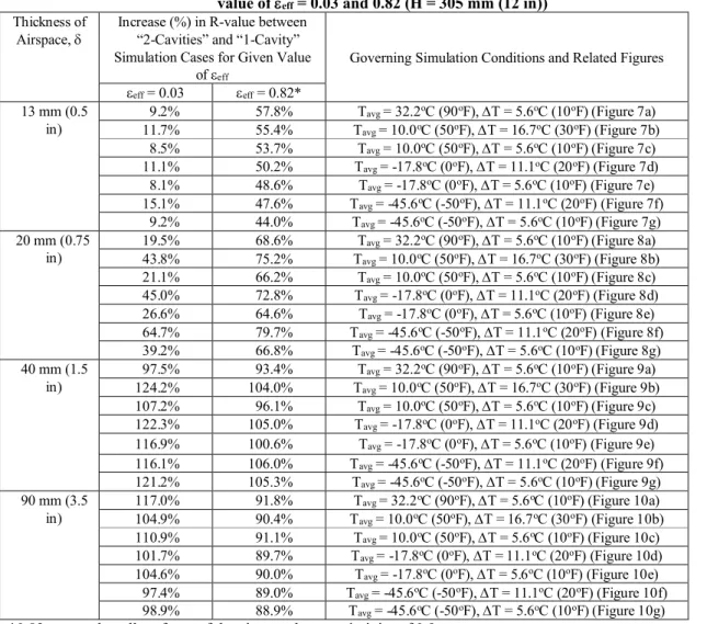
Table 2. Percentage increase in R-value between “2-Cavities” and “1-Cavity” simulation cases for given value of eff= 0.03 and 0.82 (H = 305 mm (12 in))
Thickness of
Airspace, Increase (%) in R-value between “2-Cavities” and “1-Cavity” Simulation Cases for Given Value
of eff
Governing Simulation Conditions and Related Figures eff= 0.03 eff= 0.82*
13 mm (0.5 in)
9.2% 57.8% Tavg= 32.2oC (90oF), T = 5.6oC (10oF) (Figure 7a)
11.7% 55.4% Tavg= 10.0oC (50oF), T = 16.7oC (30oF) (Figure 7b)
8.5% 53.7% Tavg= 10.0oC (50oF), T = 5.6oC (10oF) (Figure 7c)
11.1% 50.2% Tavg= -17.8oC (0oF), T = 11.1oC (20oF) (Figure 7d)
8.1% 48.6% Tavg= -17.8oC (0oF), T = 5.6oC (10oF) (Figure 7e)
15.1% 47.6% Tavg= -45.6oC (-50oF), T = 11.1oC (20oF) (Figure 7f)
9.2% 44.0% Tavg= -45.6oC (-50oF), T = 5.6oC (10oF) (Figure 7g)
20 mm (0.75 in)
19.5% 68.6% Tavg= 32.2oC (90oF), T = 5.6oC (10oF) (Figure 8a)
43.8% 75.2% Tavg= 10.0oC (50oF), T = 16.7oC (30oF) (Figure 8b)
21.1% 66.2% Tavg= 10.0oC (50oF), T = 5.6oC (10oF) (Figure 8c)
45.0% 72.8% Tavg= -17.8oC (0oF), T = 11.1oC (20oF) (Figure 8d)
26.6% 64.6% Tavg= -17.8oC (0oF), T = 5.6oC (10oF) (Figure 8e)
64.7% 79.7% Tavg= -45.6oC (-50oF), T = 11.1oC (20oF) (Figure 8f)
39.2% 66.8% Tavg= -45.6oC (-50oF), T = 5.6oC (10oF) (Figure 8g)
40 mm (1.5 in)
97.5% 93.4% Tavg= 32.2oC (90oF), T = 5.6oC (10oF) (Figure 9a)
124.2% 104.0% Tavg= 10.0oC (50oF), T = 16.7oC (30oF) (Figure 9b)
107.2% 96.1% Tavg= 10.0oC (50oF), T = 5.6oC (10oF) (Figure 9c)
122.3% 105.0% Tavg= -17.8oC (0oF), T = 11.1oC (20oF) (Figure 9d)
116.9% 100.6% Tavg= -17.8oC (0oF), T = 5.6oC (10oF) (Figure 9e)
116.1% 106.0% Tavg= -45.6oC (-50oF), T = 11.1oC (20oF) (Figure 9f)
121.2% 105.3% Tavg= -45.6oC (-50oF), T = 5.6oC (10oF) (Figure 9g)
90 mm (3.5 in)
117.0% 91.8% Tavg= 32.2oC (90oF), T = 5.6oC (10oF) (Figure 10a)
104.9% 90.4% Tavg= 10.0oC (50oF), T = 16.7oC (30oF) (Figure 10b)
110.9% 91.1% Tavg= 10.0oC (50oF), T = 5.6oC (10oF) (Figure 10c)
101.7% 89.7% Tavg= -17.8oC (0oF), T = 11.1oC (20oF) (Figure 10d)
104.6% 90.0% Tavg= -17.8oC (0oF), T = 5.6oC (10oF) (Figure 10e)
97.4% 89.0% Tavg= -45.6oC (-50oF), T = 11.1oC (20oF) (Figure 10f)
98.9% 88.9% Tavg= -45.6oC (-50oF), T = 5.6oC (10oF) (Figure 10g)
Table 3. List of the correlation coefficients given by Eq. (2) for 30osloped enclosed airspace of different thickness (δ) and subjected to downward heat flow condition
13 mm (0.5 in) 20 mm (0.75 in) 40 mm (1.5 in) 90 mm (3.5 in)
eff < 0.2 > 0.2 < 0.2 > 0.2 < 0.2 > 0.2 < 0.2 > 0.2
a0 -4.20303E+09 -3.92054E+07 -1.02535E+07 -8.07976E+05 -3.94458E+03 -1.68688E+03 -3.08298E+03 -2.15425E+03
a -3.18336E-08 -3.35999E+06 6.85455E+00 1.00733E+04 5.50178E-04 1.42662E-01 -3.27123E-02 -5.13122E-03
b1 -2.16372E-02 -1.35086E+01 -6.82661E-03 -1.08392E+00 -1.08462E-04 -2.75871E+00 -6.99787E-04 -7.41166E+01
b2 2.52195E-01 2.98545E+01 1.85466E-05 2.19043E+00 4.78370E-04 4.50290E+00 2.69448E-03 1.44100E+02
b3 -1.63207E+00 -3.52741E+01 1.18541E-01 -2.27768E+00 -1.62816E-03 -3.74561E+00 -6.98329E-03 -1.48088E+02
b4 3.66767E+00 1.59721E+01 -3.43238E-01 9.59697E-01 2.59561E-03 1.26887E+00 7.65031E-03 6.02130E+01
1 -9.77836E-01 -3.05543E-01 -3.54554E-01 -3.78040E-01 9.77418E-04 -1.19315E-01 7.02151E-02 7.81863E-04
2 -2.44453E-02 1.15288E-02 1.73155E-01 4.43617E-02 3.57088E-01 4.30360E-03 2.97140E-01 2.36302E-02
1.78199E+00 -8.05799E-01 -1.42459E-02 1.98765E+00 1.68705E-04 3.86463E-01 5.19753E-04 -8.26093E-01
a1 -4.08843E+00 -4.40061E+00 -2.86732E+00 -2.40958E+00 -1.17580E+00 -1.02878E+00 -9.41476E-01 -8.94500E-01
a2 2.61259E+00 -4.68163E+00 -1.10609E+00 -2.64682E+00 6.42540E-01 -6.12543E-01 -1.70103E-01 2.45535E-03
a3 1.17759E+00 -8.12927E-02 1.27759E+00 4.13771E-01 2.09613E+00 3.31331E-01 1.83483E+00 -2.13120E-01
c1 8.11359E-01 2.04716E+00 4.73760E-01 3.16967E-01 8.63987E-02 1.27581E-01 3.58635E-02 4.84401E-02
c2 4.10220E-01 -3.97110E-02 -2.83224E-01 -1.40695E-02 -3.13071E-01 1.62652E-01 -9.39628E-02 -1.32912E-01
c3 -5.30220E-02 -2.10464E-02 -1.97089E-01 -3.65057E-02 -3.84567E-01 -4.70174E-01 -3.42478E-01 -1.78777E-01
g1 1.09068E-01 -7.77669E+01 6.38855E-01 -8.91735E+00 1.26488E+01 -3.13988E+01 -5.11726E+01 1.58407E+01
g2 2.53419E-03 5.92793E-01 9.88143E-03 1.69700E-01 -3.12360E-01 1.31736E+00 1.97449E+00 -2.14932E+00
g3 -2.59154E-05 -1.03566E-03 -2.37003E-04 -1.38771E-03 5.19345E-03 -2.56290E-02 -4.28813E-02 1.00283E-01
1 / 2 / 1 * * eff 1 1 / 1 / 1 / 1 * eff 1 2
Gravity
= 30
oFigure 1. Schematics of sloped enclosed airspace of 30owith and without thin sheet of low emissivity on
0.5 1.0 1.5 2.0 2.5 3.0 3.5 4.0 4.5 0 0.1 0.2 0.3 0.4 0.5 0.6 0.7 0.8 0.9 (b)= 20 mm = 30o(Present) = 45o(Saber 2013d)
= 0o(Horizontal, Saber 2013e)
= 90o(Vertical, Saber 2013b) eff R -V al u e (f t 2 hr o F /B T U ) 0.5 1.0 1.5 2.0 2.5 3.0 3.5 4.0 4.5 5.0 5.5 6.0 6.5 7.0 0 0.1 0.2 0.3 0.4 0.5 0.6 0.7 0.8 0.9 (c)= 40 mm = 30o(Present) = 45o(Saber 2013d) = 0o(Horizontal) = 90o(Vertical, Saber 2013b) 0.5 1.5 2.5 3.5 4.5 5.5 6.5 7.5 8.5 9.5 0 0.1 0.2 0.3 0.4 0.5 0.6 0.7 0.8 0.9 (d)= 90 mm = 30o(Present) = 45o(Saber 2013d)
= 0o(Horizontal, Saber 2013e)
= 90o(Vertical, Saber 2013b) eff 0.8 1.0 1.2 1.4 1.6 1.8 2.0 2.2 2.4 2.6 2.8 3.0 0 0.1 0.2 0.3 0.4 0.5 0.6 0.7 0.8 0.9 (a)= 13 mm
= 0o(Horizontal, Saber 2013e) = 30o(Present) = 45o(Saber 2013d) = 90o(Vertical, Saber 2013b) R -V al ue (f t 2 hr o F /B T U )
Figure 2. Comparisons of the R-values of vertical enclosed airspaces (= 90o) with that for = 45o, 30oand 0oand subjected to downward heat
Figure 3. Temperature contours (in oC) in enclosed airspace in the cases of “1-Cavity” and
“2-Cavities” when Tavg= 10oC (50oF), T = 16.7oC (30oF), 1= 0.05, 2= 0.9, = 90 mm (3.5 in), H = 305
Y-velocity (mm)
Note: left contour bar for “1-Cavity”
and right contour bar for “2-Cavities”
Figure 4. Vertical velocity contours of the air (in mm/s) in enclosed airspace in the cases of “1-Cavity” and “2-Cavities” when Tavg= 10oC (50oF), T = 16.7oC (30oF), 1= 0.05, 2= 0.9, = 90 mm (3.5 in),
Figure 5. Temperature contours (in oC) in enclosed airspace in the cases of “1-Cavity” and
“2-Cavities” when Tavg= 10oC (50oF), T = 16.7oC (30oF), 1= 0.05, 2= 0.9, = 40 mm (1.5 in), H = 305
Note: left contour bar for “1-Cavity”
and right contour bar for “2-Cavities”
Figure 6. Vertical velocity contours of the air (in mm/s) in enclosed airspace in the cases of “1-Cavity” and “2-Cavities” when Tavg= 10oC (50oF), T = 16.7oC (30oF), 1= 0.05, 2= 0.9, = 40 mm (1.5 in),
0.5 1.0 1.5 2.0 2.5 3.0 3.5 0 0.1 0.2 0.3 0.4 0.5 0.6 0.7 0.8 0.9 7: Tavg= -45.6oC &T = 5.6oC 6: Tavg= -45.6oC &T = 11.1oC 5: Tavg= -17.8oC &T = 5.6oC 4: Tavg= -17.8oC &T = 11.1oC 3: Tavg= 10.0oC &T = 5.6oC 2: Tavg= 10.0oC &T = 16.7oC 1: Tavg= 32.2oC &T = 5.6oC
(h) 1-Cavity (different TavgandT)
eff 0.9 1.1 1.3 1.5 1.7 1.9 2.1 2.3 2.5 2.7 2.9 3.1 0 0.1 0.2 0.3 0.4 0.5 0.6 0.7 0.8 0.9 2-Cavities 1-Cavity (b) Tavg= 10.0oC,T = 16.7oC R -V a lu e (f t 2 h r o F /B T U ) 0.9 1.1 1.3 1.5 1.7 1.9 2.1 2.3 2.5 2.7 2.9 3.1 0 0.1 0.2 0.3 0.4 0.5 0.6 0.7 0.8 0.9 2-Cavities 1-Cavity (c) Tavg= 10.0oC,T = 5.6oC R -V al u e (f t 2 hr o F /B T U ) 1.0 1.2 1.4 1.6 1.8 2.0 2.2 2.4 2.6 2.8 3.0 3.2 3.4 0 0.1 0.2 0.3 0.4 0.5 0.6 0.7 0.8 0.9 2-Cavities 1-Cavity (d) Tavg= -17.8oC,T = 11.1oC eff R -V a lu e (f t 2 hr o F /B T U ) 1.0 1.2 1.4 1.6 1.8 2.0 2.2 2.4 2.6 2.8 3.0 3.2 3.4 0 0.1 0.2 0.3 0.4 0.5 0.6 0.7 0.8 0.9 2-Cavities 1-Cavity (e) Tavg= -17.8oC,T = 5.6oC 1.4 1.6 1.8 2.0 2.2 2.4 2.6 2.8 3.0 3.2 3.4 3.6 3.8 0 0.1 0.2 0.3 0.4 0.5 0.6 0.7 0.8 0.9 2-Cavities 1-Cavity (f) Tavg= -45.6oC,T = 11.1oC 1.4 1.6 1.8 2.0 2.2 2.4 2.6 2.8 3.0 3.2 3.4 3.6 3.8 0 0.1 0.2 0.3 0.4 0.5 0.6 0.7 0.8 0.9 2-Cavities 1-Cavity (g) Tavg= -45.6oC,T = 5.6oC 0.6 0.8 1.0 1.2 1.4 1.6 1.8 2.0 2.2 2.4 2.6 2.8 0 0.1 0.2 0.3 0.4 0.5 0.6 0.7 0.8 0.9 2-Cavities 1-Cavity (a) Tavg= 32.2oC,T = 5.6oC R -V a lu e (f t 2 hr o F /B T U )
0.5 1.0 1.5 2.0 2.5 3.0 3.5 4.0 4.5 0 0.1 0.2 0.3 0.4 0.5 0.6 0.7 0.8 0.9 2-Cavities 1-Cavity (b) Tavg= 10.0oC,T = 16.7oC R -V a lu e (f t 2 hr o F /B T U ) 1.0 1.5 2.0 2.5 3.0 3.5 4.0 4.5 0 0.1 0.2 0.3 0.4 0.5 0.6 0.7 0.8 0.9 2-Cavities 1-Cavity (c) Tavg= 10.0oC,T = 5.6oC R -V a lu e (f t 2 h r o F /B T U ) 1.0 1.5 2.0 2.5 3.0 3.5 4.0 4.5 5.0 0 0.1 0.2 0.3 0.4 0.5 0.6 0.7 0.8 0.9 2-Cavities 1-Cavity (d) Tavg= -17.8oC,T = 11.1oC eff R -V al ue (f t 2 hr o F /B T U ) 1.0 1.5 2.0 2.5 3.0 3.5 4.0 4.5 5.0 0 0.1 0.2 0.3 0.4 0.5 0.6 0.7 0.8 0.9 2-Cavities 1-Cavity (e) Tavg= -17.8oC,T = 5.6oC 1.5 2.0 2.5 3.0 3.5 4.0 4.5 5.0 5.5 0 0.1 0.2 0.3 0.4 0.5 0.6 0.7 0.8 0.9 2-Cavities 1-Cavity (f) Tavg= -45.6oC,T = 11.1oC 1.5 2.0 2.5 3.0 3.5 4.0 4.5 5.0 5.5 0 0.1 0.2 0.3 0.4 0.5 0.6 0.7 0.8 0.9 2-Cavities 1-Cavity (g) Tavg= -45.6oC,T = 5.6oC 0.5 1.0 1.5 2.0 2.5 3.0 3.5 4.0 4.5 0 0.1 0.2 0.3 0.4 0.5 0.6 0.7 0.8 0.9 7: Tavg= -45.6oC &T = 5.6oC 6: Tavg= -45.6oC &T = 11.1oC 5: Tavg= -17.8oC &T = 5.6oC 4: Tavg= -17.8oC &T = 11.1oC 3: Tavg= 10.0oC &T = 5.6oC 2: Tavg= 10.0oC &T = 16.7oC 1: Tavg= 32.2oC &T = 5.6oC
(h) 1-Cavity (different TavgandT)
eff 0.5 1.0 1.5 2.0 2.5 3.0 3.5 4.0 4.5 0 0.1 0.2 0.3 0.4 0.5 0.6 0.7 0.8 0.9 2-Cavities 1-Cavity (a) Tavg= 32.2oC,T = 5.6oC R -V a lu e (f t 2 h r o F /B T U )
1 2 3 4 5 6 7 8 0 0.1 0.2 0.3 0.4 0.5 0.6 0.7 0.8 0.9 2-Cavities 1-Cavity (d) Tavg= -17.8oC,T = 11.1oC eff R -V al ue (f t 2 hr o F /B T U ) 1 2 3 4 5 6 7 8 9 0 0.1 0.2 0.3 0.4 0.5 0.6 0.7 0.8 0.9 2-Cavities 1-Cavity (c) Tavg= 10.0oC,T = 5.6oC R -V al ue (f t 2 hr o F /B T U ) 1 2 3 4 5 6 7 8 9 0 0.1 0.2 0.3 0.4 0.5 0.6 0.7 0.8 0.9 2-Cavities 1-Cavity (e) Tavg= -17.8oC,T = 5.6oC 0.5 1.0 1.5 2.0 2.5 3.0 3.5 4.0 4.5 0 0.1 0.2 0.3 0.4 0.5 0.6 0.7 0.8 0.9 7: Tavg= -45.6oC &T = 5.6oC 6: Tavg= -45.6oC &T = 11.1oC 5: Tavg= -17.8oC &T = 5.6oC 4: Tavg= -17.8oC &T = 11.1oC 3: Tavg= 10.0oC &T = 5.6oC 2: Tavg= 10.0oC &T = 16.7oC 1: Tavg= 32.2oC &T = 5.6oC
(h) 1-Cavity (different TavgandT)
eff 1 2 3 4 5 6 7 8 9 0 0.1 0.2 0.3 0.4 0.5 0.6 0.7 0.8 0.9 2-Cavities 1-Cavity (g) Tavg= -45.6oC,T = 5.6oC 1 2 3 4 5 6 7 8 0 0.1 0.2 0.3 0.4 0.5 0.6 0.7 0.8 0.9 2-Cavities 1-Cavity (b) Tavg= 10.0oC,T = 16.7oC R -V al ue (f t 2 hr o F /B T U ) 1 2 3 4 5 6 7 8 0 0.1 0.2 0.3 0.4 0.5 0.6 0.7 0.8 0.9 2-Cavities 1-Cavity (f) Tavg= -45.6oC,T = 11.1oC 0 1 2 3 4 5 6 7 8 0 0.1 0.2 0.3 0.4 0.5 0.6 0.7 0.8 0.9 2-Cavities 1-Cavity (a) Tavg= 32.2oC,T = 5.6oC R -V al ue (f t 2 hr o F /B T U )
1 2 3 4 5 6 7 8 9 10 0 0.1 0.2 0.3 0.4 0.5 0.6 0.7 0.8 0.9 2-Cavities 1-Cavity (g) Tavg= -45.6oC,T = 5.6oC 1 2 3 4 5 6 7 8 9 0 0.1 0.2 0.3 0.4 0.5 0.6 0.7 0.8 0.9 2-Cavities 1-Cavity (f) Tavg= -45.6oC,T = 11.1oC 1 2 3 4 5 6 7 8 9 10 0 0.1 0.2 0.3 0.4 0.5 0.6 0.7 0.8 0.9 2-Cavities 1-Cavity (e) Tavg= -17.8oC,T = 5.6oC 1 2 3 4 5 6 7 8 0 0.1 0.2 0.3 0.4 0.5 0.6 0.7 0.8 0.9 2-Cavities 1-Cavity (b) Tavg= 10.0oC,T = 16.7oC R -V al ue (f t 2 hr o F /B T U ) 1 2 3 4 5 6 7 8 9 10 0 0.1 0.2 0.3 0.4 0.5 0.6 0.7 0.8 0.9 2-Cavities 1-Cavity (c) Tavg= 10.0oC,T = 5.6oC R -V a lu e (f t 2 h r o F /B T U ) 1 2 3 4 5 6 7 8 9 0 0.1 0.2 0.3 0.4 0.5 0.6 0.7 0.8 0.9 2-Cavities 1-Cavity (d) Tavg= -17.8oC,T = 11.1oC eff R -V al ue (f t 2 h r o F /B T U ) 0.5 1.0 1.5 2.0 2.5 3.0 3.5 4.0 4.5 5.0 0 0.1 0.2 0.3 0.4 0.5 0.6 0.7 0.8 0.9 7: Tavg= -45.6oC &T = 5.6oC 6: Tavg= -45.6oC &T = 11.1oC 5: Tavg= -17.8oC &T = 5.6oC 4: Tavg= -17.8oC &T = 11.1oC 3: Tavg= 10.0oC &T = 5.6oC 2: Tavg= 10.0oC &T = 16.7oC 1: Tavg= 32.2oC &T = 5.6oC
(h) 1-Cavity (different TavgandT)
eff 0 1 2 3 4 5 6 7 8 9 10 0 0.1 0.2 0.3 0.4 0.5 0.6 0.7 0.8 0.9 2-Cavities 1-Cavity (a) Tavg= 32.2oC,T = 5.6oC R -V a lu e (f t 2 h r o F /B T U )
0.9 1.1 1.3 1.5 1.7 1.9 2.1 2.3 2.5 2.7 2.9 3.1 0 0.1 0.2 0.3 0.4 0.5 0.6 0.7 0.8 0.9 H = 96" 72" 48" 36" 24" 16" 12" 8" (c) Tavg= 10.0oC,T = 5.6oC R -V al u e (f t 2 h r o F /B T U ) 1.0 1.2 1.4 1.6 1.8 2.0 2.2 2.4 2.6 2.8 3.0 3.2 3.4 0 0.1 0.2 0.3 0.4 0.5 0.6 0.7 0.8 0.9 H = 96" 72" 48" 36" 24" 16" 12" 8" (d) Tavg= -17.8oC,T = 11.1oC eff R -V a lu e (f t 2 hr o F /B T U ) 1.4 1.6 1.8 2.0 2.2 2.4 2.6 2.8 3.0 3.2 3.4 3.6 0 0.1 0.2 0.3 0.4 0.5 0.6 0.7 0.8 0.9 H = 96" 72" 48" 36" 24" 16" 12" 8" (f) Tavg= -45.6oC,T = 11.1oC 1.4 1.6 1.8 2.0 2.2 2.4 2.6 2.8 3.0 3.2 3.4 3.6 0 0.1 0.2 0.3 0.4 0.5 0.6 0.7 0.8 0.9 H = 96" 72" 48" 36" 24" 16" 12" 8" (g) Tavg= -45.6oC,T = 5.6oC 1.0 1.2 1.4 1.6 1.8 2.0 2.2 2.4 2.6 2.8 3.0 3.2 3.4 0 0.1 0.2 0.3 0.4 0.5 0.6 0.7 0.8 0.9 H = 96" 72" 48" 36" 24" 16" 12" 8" (e) Tavg= -17.8oC,T = 5.6oC 0.9 1.1 1.3 1.5 1.7 1.9 2.1 2.3 2.5 2.7 2.9 3.1 0 0.1 0.2 0.3 0.4 0.5 0.6 0.7 0.8 0.9 H = 96" 72" 48" 36" 24" 16" 12" 8" (b) Tavg= 10.0oC,T = 16.7oC R -V a lu e (f t 2 h r o F /B T U ) 0.5 1.0 1.5 2.0 2.5 3.0 3.5 4.0 0 0.1 0.2 0.3 0.4 0.5 0.6 0.7 0.8 0.9
(h) All cases (different TavgandT)
eff 0.6 0.8 1.0 1.2 1.4 1.6 1.8 2.0 2.2 2.4 2.6 2.8 0 0.1 0.2 0.3 0.4 0.5 0.6 0.7 0.8 0.9 H = 96" 72" 48" 36" 24" 16" 12" 8" (a) Tavg= 32.2oC,T = 5.6oC R -V al u e (f t 2 hr o F /B T U )
0.5 1.0 1.5 2.0 2.5 3.0 3.5 4.0 4.5 0 0.1 0.2 0.3 0.4 0.5 0.6 0.7 0.8 0.9 H = 96" 72" 48" 36" 24" 16" 12" 8" (b) Tavg= 10.0oC,T = 16.7oC R -V a lu e (f t 2 h r o F /B T U ) 1.0 1.5 2.0 2.5 3.0 3.5 4.0 4.5 0 0.1 0.2 0.3 0.4 0.5 0.6 0.7 0.8 0.9 H = 96" 72" 48" 36" 24" 16" 12" 8" (c) Tavg= 10.0oC,T = 5.6oC R -V al u e (f t 2 hr o F /B T U ) 1.0 1.5 2.0 2.5 3.0 3.5 4.0 4.5 5.0 0 0.1 0.2 0.3 0.4 0.5 0.6 0.7 0.8 0.9 H = 96" 72" 48" 36" 24" 16" 12" 8" (d) Tavg= -17.8oC,T = 11.1oC eff R -V a lu e (f t 2 hr o F /B T U ) 1.0 1.5 2.0 2.5 3.0 3.5 4.0 4.5 5.0 0 0.1 0.2 0.3 0.4 0.5 0.6 0.7 0.8 0.9 H = 96" 72" 48" 36" 24" 16" 12" 8" (e) Tavg= -17.8oC,T = 5.6oC 1.0 1.5 2.0 2.5 3.0 3.5 4.0 4.5 5.0 0 0.1 0.2 0.3 0.4 0.5 0.6 0.7 0.8 0.9 H = 96" 72" 48" 36" 24" 16" 12" 8" (f) Tavg= -45.6oC,T = 11.1oC 1.5 2.0 2.5 3.0 3.5 4.0 4.5 5.0 5.5 0 0.1 0.2 0.3 0.4 0.5 0.6 0.7 0.8 0.9 H = 96" 72" 48" 36" 24" 16" 12" 8" (g) Tavg= -45.6oC,T = 5.6oC 0.5 1.0 1.5 2.0 2.5 3.0 3.5 4.0 4.5 5.0 5.5 0 0.1 0.2 0.3 0.4 0.5 0.6 0.7 0.8 0.9
(h) All cases (different TavgandT)
eff 0.5 1.0 1.5 2.0 2.5 3.0 3.5 4.0 4.5 0 0.1 0.2 0.3 0.4 0.5 0.6 0.7 0.8 0.9 H = 96" 72" 48" 36" 24" 16" 12" 8" (a) Tavg= 32.2oC,T = 5.6oC R -V a lu e (f t 2 hr o F /B T U )
1.0 1.5 2.0 2.5 3.0 3.5 4.0 4.5 5.0 5.5 0 0.1 0.2 0.3 0.4 0.5 0.6 0.7 0.8 0.9 H = 96" 60" 48" 36" 24" 16" 12" 8" (d) Tavg= -17.8oC,T = 11.1oC eff R -V a lu e (f t 2 h r o F /B T U ) 1.0 1.5 2.0 2.5 3.0 3.5 4.0 4.5 5.0 5.5 6.0 6.5 0 0.1 0.2 0.3 0.4 0.5 0.6 0.7 0.8 0.9 H = 96" 60" 48" 36" 24" 16" 12" 8" (e) Tavg= -17.8oC,T = 5.6oC 1.5 2.0 2.5 3.0 3.5 4.0 4.5 5.0 5.5 0 0.1 0.2 0.3 0.4 0.5 0.6 0.7 0.8 0.9 H = 72" 60" 48" 36" 24" 16" 12" 8" (f) Tavg= -45.6oC,T = 11.1oC 1.5 2.0 2.5 3.0 3.5 4.0 4.5 5.0 5.5 6.0 0 0.1 0.2 0.3 0.4 0.5 0.6 0.7 0.8 0.9 H = 96" 60" 48" 36" 24" 16" 12" 8" (g) Tavg= -45.6oC,T = 5.6oC 0.5 1.0 1.5 2.0 2.5 3.0 3.5 4.0 4.5 5.0 5.5 6.0 6.5 0 0.1 0.2 0.3 0.4 0.5 0.6 0.7 0.8 0.9
(h) All cases (different TavgandT)
eff 1.0 1.5 2.0 2.5 3.0 3.5 4.0 4.5 5.0 0 0.1 0.2 0.3 0.4 0.5 0.6 0.7 0.8 0.9 H = 96" 60" 48" 36" 24" 16" 12" 8" (b) Tavg= 10.0oC,T = 16.7oC R -V al ue (f t 2 hr o F /B T U ) 1.0 1.5 2.0 2.5 3.0 3.5 4.0 4.5 5.0 5.5 6.0 6.5 0 0.1 0.2 0.3 0.4 0.5 0.6 0.7 0.8 0.9 H = 96" 60" 48" 36" 24" 16" 12" 8" (c) Tavg= 10.0oC,T = 5.6oC R -V al u e (f t 2 hr o F /B T U ) 0.5 1.0 1.5 2.0 2.5 3.0 3.5 4.0 4.5 5.0 5.5 6.0 6.5 0 0.1 0.2 0.3 0.4 0.5 0.6 0.7 0.8 0.9 H = 96" 60" 48" 36" 24" 16" 12" 8" (a) Tavg= 32.2oC,T = 5.6oC R -V al u e (f t 2 hr o F /B T U )
1.0 1.5 2.0 2.5 3.0 3.5 4.0 4.5 5.0 5.5 0 0.1 0.2 0.3 0.4 0.5 0.6 0.7 0.8 0.9 H = 96" 72" 60" 48" 36" 24" 16" 12" 8" (b) Tavg= 10.0oC,T = 16.7oC R -V a lu e (f t 2 h r o F /B T U ) 1.0 1.5 2.0 2.5 3.0 3.5 4.0 4.5 5.0 5.5 6.0 6.5 7.0 0 0.1 0.2 0.3 0.4 0.5 0.6 0.7 0.8 0.9 H = 96" 72" 60" 48" 36" 24" 16" 12" 8" (c) Tavg= 10.0oC,T = 5.6oC R -V al u e (f t 2 hr o F /B T U ) 1.0 1.5 2.0 2.5 3.0 3.5 4.0 4.5 5.0 5.5 6.0 0 0.1 0.2 0.3 0.4 0.5 0.6 0.7 0.8 0.9 H = 96" 72" 60" 48" 36" 24" 16" 12" 8" (d) Tavg= -17.8oC,T = 11.1oC eff R -V a lu e (f t 2 hr o F /B T U ) 1.5 2.0 2.5 3.0 3.5 4.0 4.5 5.0 5.5 0 0.1 0.2 0.3 0.4 0.5 0.6 0.7 0.8 0.9 H = 96" 72" 60" 48" 36" 24" 16" 12" 8" (f) Tavg= -45.6oC,T = 11.1oC 1.0 1.5 2.0 2.5 3.0 3.5 4.0 4.5 5.0 5.5 6.0 6.5 7.0 0 0.1 0.2 0.3 0.4 0.5 0.6 0.7 0.8 0.9 H = 96" 72" 60" 48" 36" 24" 16" 12" 8" (e) Tavg= -17.8oC,T = 5.6oC 1.5 2.0 2.5 3.0 3.5 4.0 4.5 5.0 5.5 6.0 6.5 0 0.1 0.2 0.3 0.4 0.5 0.6 0.7 0.8 0.9 H = 96" 72" 60" 48" 36" 24" 16" 12" 8" (g) Tavg= -45.6oC,T = 5.6oC 0.5 1.0 1.5 2.0 2.5 3.0 3.5 4.0 4.5 5.0 5.5 6.0 6.5 7.0 0 0.1 0.2 0.3 0.4 0.5 0.6 0.7 0.8 0.9
(h) All cases (different TavgandT)
eff 0.5 1.0 1.5 2.0 2.5 3.0 3.5 4.0 4.5 5.0 5.5 6.0 6.5 7.0 0 0.1 0.2 0.3 0.4 0.5 0.6 0.7 0.8 0.9 H = 96" 60" 48" 36" 24" 16" 12" 8" (a) Tavg= 32.2oC,T = 5.6oC R -V a lu e (f t 2 hr o F /B T U )
0.5 1.0 1.5 2.0 2.5 3.0 3.5 4.0 4.5 5.0 5.5 0.5 1.0 1.5 2.0 2.5 3.0 3.5 4.0 4.5 5.0 5.5
All Cases:eff< 0.2 All Cases:eff0.2 +3% -3% (b)= 20 mm R (ft2hroF/BTU) RC o rr el a tio n (f t 2 hr o F /B T U ) 0.5 1.0 1.5 2.0 2.5 3.0 3.5 4.0 4.5 5.0 5.5 6.0 6.5 7.0 0.5 1.0 1.5 2.0 2.5 3.0 3.5 4.0 4.5 5.0 5.5 6.0 6.5 7.0 All Cases:eff< 0.2 All Cases:eff0.2 +3% -3% (d)= 90 mm R (ft2hroF/BTU) 0.5 1.0 1.5 2.0 2.5 3.0 3.5 4.0 4.5 5.0 5.5 6.0 6.5 0.5 1.0 1.5 2.0 2.5 3.0 3.5 4.0 4.5 5.0 5.5 6.0 6.5 All Cases:eff< 0.2
All Cases:eff0.2 +3% -3% (c)= 40 mm 0.5 1.0 1.5 2.0 2.5 3.0 3.5 4.0 0.5 1.0 1.5 2.0 2.5 3.0 3.5 4.0
All Cases:eff< 0.2 All Cases:eff0.2 +3% -3% (a)= 13 mm RC or re la tio n (f t 2 hr o F /B T U )