Biomechanical Changes to Human Locomotion
Due to Asymmetric Loading of the Legs
by
Wesley D. McDougal
Submitted to the
Department of Mechanical Engineering
in Partial Fulfillment of the Requirements for the Degree of
Bachelor of Science in Mechanical Engineering
at the
Massachusetts Institute of Technology
June 2012
ARCHIVES
MASS6ACHUSETTS INSTITUT5. OF TECHNOLOGYJUN 28 2012
LIBRARIES
@ 2012 Wesley D. McDougal. All rights reserved.
The author hereby grants to MIT permission to reproduce and to distribute
publicly paper and electronic copies of this thesis document in whole
or in part in any medium now known or hereafter created.
Signature of Author:
Department of Mechanical Engineering
May 18, 2012
Certified by:
Accepted by:
Neville Hogan
Sun Jae Professor of Mechanical Engineering
Thesis SupervisorJohin H. Lienhard V
Samuel C. Collins
echanical Engineering
Biomechanical Changes to Human Locomotion Due to Asymmetric Loading
byWesley D. McDougal
Submitted to the Department of Mechanical Engineering on May 18, 2012 in Partial Fulfillment of the
Requirements for the Degree of
Bachelor of Science in Mechanical Engineering
ABSTRACT
The biomechanics of lower limb locomotion is a yet unknown mixture of neurological control and physical parameters. The current study explored attaching a rehabilitative anklebot to subjects walking on a treadmill and observed duration, kinematic, and electromyography data to determine the biomechanical response to the asymmetric loading.
The present report identified various gait cycle parameters that changed as a response to the asymmetric loading. Notably, significant differences in the stride time of the legs occurred under loading, while contralateral stride times also adjusted to remain equal to those of the loaded legs.
Symmetry index analysis led to the conclusion that, while the asymmetric loading of the lower limbs had some effects on temporal gait parameters, the body adjusted to minimize any temporal asymmetry. However, goniometer data demonstrated kinematic changes in response to loading as knee flexion peaked earlier in the gait cycle.
Thesis Supervisor: Neville Hogan
Acknowledgements
This work, and MIT in general has been a massive learning process, and I want to give thanks to everyone who has helped me throughout the experience.
First I want to thank Prof. Hogan for his oversight, guidance, and thoughtful, patient critique of the thesis process. I really learned this semester, and thank you for helping me in that process.
Also Hyunglae - thanks for spending so much time making sure I knew what I was doing and was doing it right. The ideas and guidance you provided were invaluable. Shuo, thanks for showing me the ropes around the lab.
Thanks to my friends, who helped me when I got stuck on analysis, looked at MATLAB code with me, and fake limped all around the house and campus so I could think about asymmetry. Thank you all for providing the daily encouragement and support that the project needed.
Finally, thanks to my amazing family and their eternal support, especially to my parents, who started the learning journey with me and now get to finish the official schooling process with me. The eternal reminders and support have been a bigger blessing than I can describe.
Table of Contents
Abstract 3 Acknowledgements 5 Table of Contents 7 List of Figures 8 List of Tables 9 1. Introduction 11 2. Details/Experimental Setup 13 2.1 Overview 13 2.2 Apparatus 13 2.3 Subjects 14 2.4 Experimental Methods 14 3. Data Analysis 18 3.1 Duration 18 3.2 Kinematics 19 3.3 Muscle Activity 20 3.4 Statistics 21 4. Results 21 4.1 Duration 21 4.2 Kinematics 24 4.3 EMG Activity 25 5. Conclusion 26 6. Future Works 27 7. Appendices 29Appendix A: Goniometer Calibration Methods 29
Appendix B: Usable Data 31
Appendix C: Sample Code for Data Processing 32
List of Figures
Figure 1: Experimental Apparatus Components 16
Figure 2: Experimental Setup 17
Figure 3: Gait Cycle Ankle and Knee Angles 20 Figure 4: Gait Cycle EMG Response for Tibialis Anterior and Gastrocnemius 21 Figure 5: SolidWorks* Angle Sheet for Calibration 29
Figure 6: Sample Goniometer Calibration Voltage Output 30
List of Tables
TABLE 1: Subject Biographical and Physiological Data 13
TABLE 2: Mean Duration and Symmetry Parameters 23
TABLE 3: Contralateral (Loaded/Unloaded) Heel Strike Timing 24
TABLE 4: Peak Knee Flexion Timing 25
TABLE 5: Mean EMG Output per Stride 26
1.Introduction
The effects of asymmetric loading of the lower limbs is of great importance to both biomedical researchers hoping to restore normal human gait and to biomechanics researchers searching to better understand the neurological control of walking that the nervous system exerts in human locomotion. Although many studies have investigated the effects of weight-loading the lower limbs, the complete kinematics and neurological control of the locomotion system are not fully understood.
In the biomedical field, the effects of asymmetric loading of the lower limbs are of particular importance for lower limb prosthesis and orthosis users. In particular, the need to understand the effects of and training for lower limb ambulatory devices is crucial for the well-being of the users, both to minimize health risks and improve the overall quality of life for the subject (1). One primary influence on the gait cycle is the loading of the lower limbs; this factor is the subject of a great deal of study for lower limb prosthetics (2).
For researchers investigating the neural control of movement, the reaction of the lower limbs to loading could provide deeper insight to a field where, although much research has been done, there is still a great deal of uncertainty about the workings and organization of the neural control system (3)(4). While looking at the control of lower limb locomotion under loading may not yield a complete description of the neural control system, the loading's effect on lower limbs may answer critical questions about the control and regulation of walking.
Finally, the results of asymmetric loading are of particular importance to stroke patients using lower limb rehabilitation robots to aid with impaired locomotion. Stroke patients form a substantial portion of the United States population, with approximately 795,00 stroke victims each year (5). Although then number of deaths from strokes has been dropping over the last few years, the number of incidents with residual motor deficits is still staggering, with 50% of stroke survivors over the age of 65 struggling with hemiparesis (5).
This proliferation of stroke survivors with motor-deficit has led to the development of medical robots to assist with locomotion retraining. There are several available robotic assisted gait therapy
devices, from exoskeletons such as the Lokomat, AutoAmbulator, and LOPES, to moveable footplates such as Gait Trainer I and the Haptic Walker (6). With such devices, a primary concern is the propensity to preclude or at least disrupt preclude normal walking (7). Several studies have shown that robotic loading of hemiparetic patients leads to changes in kinematics (7), but the complete nature of disturbed motion introduced by the loading is yet to be fully characterized.
A recent study by Khanna et al. (2010) sought to ascertain the effects of asymmetrically loading hemiparetic subjects with an unpowered ankle robot. While they found slight variations in the kinematics of the leg, specifically reduction in nonparetic peak knee flexion during treadmill walking, there were no observable changes in the symmetry of the stroke survivor (7). However, this is not the output one would expect, because if the physical parameters of the system changed, one would also expect corresponding biomechanical changes. Thus, under the influence of a physical change such as loading, it follows that either the duration, kinematic, or muscle output parameters would adjust to retain walking performance.
As such, several questions remain from the Khanna et al. study. In particular, their investigation looked at subjects with significant hemiparesis; this impairment affected their walking speed, shortened the number of strides available for measurement, necessitated handrail used to help support body weight, and predisposed subjects display significant asymmetry between the paretic and nonparetic legs before loading (7).
For this paper, the author investigated the biomechanical effects of asymmetrically loading a single lower limb. The study strove to further investigate the results reported by Khanna et al. by examining healthy, young subjects, thereby isolating the effects of the robotic loading of the leg. In addition, this study incorporated observations of the EMG activity of the legs, while retaining observations of the kinematics and temporal aspects of the gait cycle.
2. Details/Experimental Setup
2.1 Overview
Healthy subjects were asked to walk on a treadmill for 2 ten minute intervals. They alternated between unloaded, normal walking, and asymmetric loading of a single limb using an unpowered robot
Foot switches, goniometers, and electromyography (EMG) sensors were used to record data.
2.2
Apparatus
The effects of loading were achieved by attaching an unpowered ankle robot to the knee of the subjects. This study used MIT's Anklebot, the same anklebot used by Khanna et al. Developed for the dual purpose of assisting in the rehabilitation of stroke survivors and characterizing ankle properties, the anklebot exhibits low mechanical impedance with minimal friction and backdrivability. Weighing approximately 3.6 Kg, the robot possesses 3 degrees of freedom, which allowed subjects to demonstrate the full range of motion required for locomotion (8). The anklebot was attached to the leg through a
a specialty knee-brace and specialty shoes with u-brackets for support.
The variables of walking observed were the kinematics, heel strike moment, and EMG activity of selected leg muscles. The kinematics were recorded through single axis, fiber optic goniometers from Delsys* biosignal sensors. The sensors were calibrated by positioning the goniometers at known angles and recording the output voltage." Unfortunately, the performance of these goniometers left much to be desired, as repeated trials revealed an output with extremely low precision.
Foot switches from Delsys@' biosignal sensor selection were employed to determine the moment of heel strike. The Delsys Surface EMG sensors were also used to record muscle activation data. All data were captured through a DelsysMyomonitor@ IV Wireless Transmission & Datalogging System.
aSee Figure 2(b)
2.3 Subjects
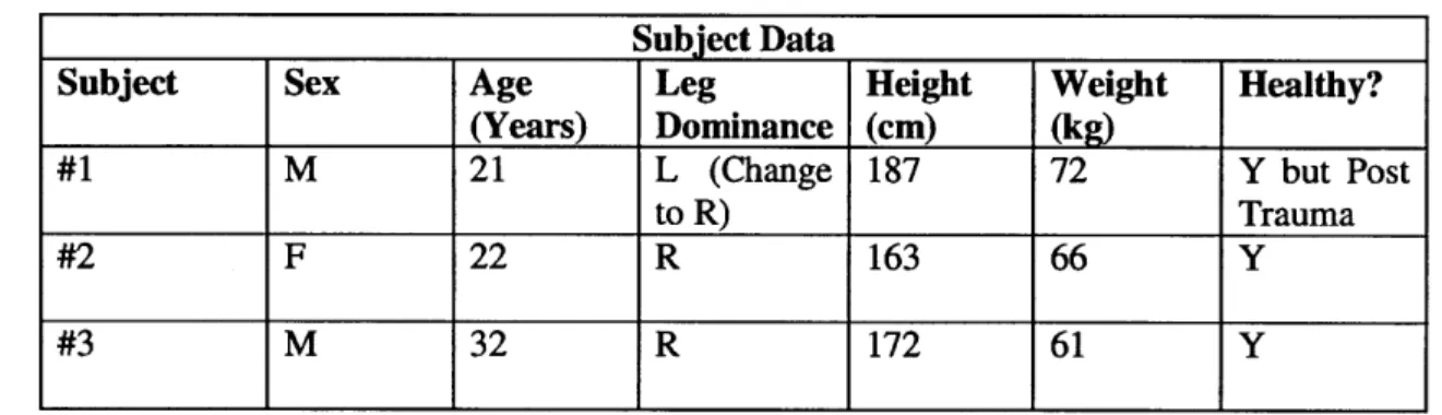
The subjects for this study were young, healthy adults, 2 male and 1 female. However, it must be noted that Subject 1 reported a traumatic injury to the dominant knee two years previously. He also self-reported a return to normal gait since the injury. Therefore, the anklebot was tested upon Subject l's non-dominant leg (henceforth called the "non-dominant leg" for consistency across all subjects).
Other biographical and physical information can be found in Table 1. All subjects volunteered to participate in the study and signed consent forms as approved by MIT's Committee on the Use of Humans as Experimental Subjects.
TABLE 1: Subject Biographical and Physiological Data
Subject Data
Subject Sex Age Leg Height Weight Healthy?
(Years) Dominance (cm) (kg)
#1 M 21 L (Change 187 72 Y but Post
to R) Trauma
#2 F 22 R 163 66 Y
#3 M 32 R 172 61 Y
2.4 Experimental Methods
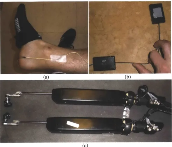
The experiment was setup and run by the author and lab research supervisors, who helped attach the sensors to the subject. The foot switches were first placed beneath the calcaneus, on the center of the subjects' heels (beneath their socks).
The knee and ankle goniometers were then carefully attached. Subjects 1 and 2 used standard medical tape as attachment mechanisms, while Subject 3 had the back of the goniometers outfitted with double sided Scotch@ Mounting Tape. We strongly recommend further use of the mounting tape, as it created a much more stable attachment method as well as improved patient comfort (by significantly reducing the amount of medical tape required).
When attaching the goniometer to the knee, care was taken to ensure that the goniometer was still flexed when the knee reached full extension in order to avoid passing through the fully extended configuration of the goniometer. The goniometer was attached to the ventral side of the knee to measure sagittal plane motion, with care being taken in the placement to ensure that the knee brace for the anklebot could fit over the goniometer without disrupting the position of the sensor. In addition, care was taken to place the center of the goniometer over the middle of the knee (lower edge of the patella) to try and obtain the best and most consistent output readings.
The ankle goniometer was attached with tape as well, once again trying to ensure that the center of the goniometer passed through the center of rotation of the ankle. However, in the loaded condition, the
strap on the anklebot shoe was also tightened around the goniometer to ensure position reinforcement.
(a) (b)
(C)
Figure 1: (a) The attachment of the foot switch below the sock. (b) The goniometer being held at a right angle along its rotation axis. Double sided mounting tape is seen on the upper-right hand block. (c) The unmounted anklebot apparatus lain horizontally on the ground. The wired end (right end in figure) was attached to the knee brace using the bracket spanning the gap, while the lower extensions (left side) attach to the anklebot shoe.
3. Data Analysis
Each 10 minute test produced over 470 strides (the shortened test for Subject 2's loaded condition produced 293 strides). The files were sent to EMGworks@ Acquisition program, and converted to text files to be processed in using Matlab@ (MathWorks@, Inc.).
3.1 Duration
The foot switch and ankle goniometer for each leg were analyzed to provide duration data for gait cycle parameters. Moment of heel strike and stride duration (time between successive heel strikes of a given leg) were determined from the foot switch. Due to the limited number of sensor collection ports, no foot switch was used on the toe. However, toe-off was estimated using the ankle trajectory; the maximum
ankle plantarflexion measurement was assumed to correspond to toe-off (9).
With the heel strike and estimated toe-off data, the duration of the stance phase (the period of gait from heel strike to toe-off) and its percent of whole gait cycle were calculated for both legs in both the loaded and unloaded conditions. In addition, a symmetry index was used to compare the dominant and non-dominant legs' percent stance phase. Employing the definition of symmetry used by Khanna et al. (2010), the symmetry index compares the percent stance phase symmetry between the left and right legs:
SI = 1* vdominant - vnon-dominant
2 Vdominant+Vnon-dominant
I
where SI varies between 0 and 1, and V is the percent stance phase for a given leg. A lower value of SI indicates a greater symmetry (a zero value for SI indicates perfect symmetry).
In addition, the time between contralateral heel strikes was calculated from the foot switch data in order to determine the relative timing of the steps. This timing was defined as the time elapsed between dominant (or loaded) leg heel strike and non-dominant heel strike. In addition, this timing between heel strikes was evaluated as a percent of the entire gait cycle duration in order to observe any phase shift in the loading condition.
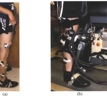
(a) (b)
Figure 2: (a) Sensor setup of the dominant leg, including the goniometers, emg sensors, and foot switch. (b) Entire loaded configuration setup, with sensors and anklebot apparatus attached.
The EMG sensors were then applied to the quadriceps (rectus femoris), hamstrings (biceps femoris long head), tibialis anterior, and gastrocnemius muscles on both legs. Finally, a ground reference pad was attached to the knee cap. With the entire measurement system attached and in place, the subject was asked to walk on the treadmill and to pick a comfortable walking speed. Once the subject reached a speed they felt comfortable with, data collection started and continued for 10 minutes.d
The subject was then stopped and asked to place the anklebot knee-brace and robot over the sensors on the dominant leg. If the subject felt that the anklebot was unsecure on their leg, he was given a form of shoulder strap or harness support to help keep the anklebot in place and support the weight of the anklebot. The subject was then asked to walk on treadmill, quickly building up to the velocity previously used, and the ten minute trial was run again.
3.2 Kinematics
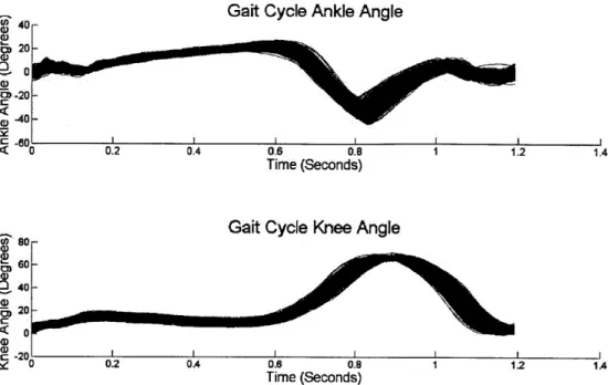
The knee and ankle goniometer data from both legs were separated into individual gaits, normalized to the mean stride time, and overlaid to observe timing and amplitude patterns. The bias was removed from the results of both the ankle and knee data. The knee data was adjusted to reset the fully extended knee (straight - no hyperextension assumed) to zero degrees, with increasing flexion corresponding to an increasing angle. Meanwhile, the bias in the ankle data was removed by adjusting initial heel strike to zero degrees, with positive angles corresponding to dorsiflexion and negative angles corresponding to plantarflexion.
However, several of the goniometer output results yielded data that appeared to fall well beyond the biomechanical limits of feasible motion in walking. Thus, further analysis of the magnitude of peak angles in the knee and ankle's gait cycle was deferred to future investigation. In addition, the knee goniometers occasionally displayed saturation, making it impossible to clearly identify the peaks.
However, despite the issues with the scaling of the goniometers, they retained significant precision and accuracy in their temporal reliability, and as such the timing of peak angle occurrence could be compared in the loaded and unloaded conditions for both the ankle and knee. The un-normalized data was overlaid and the timing of the peak knee flexion and ankle plantarflexion were determined and expressed as a percent of the total gait cycle. This timing of peak ankle plantarflexion was used as the estimated toe-off point.
Gait Cycle Ankle Angle 4) 0 0 < 0 02 0.4 0. 0.o 1 12 1.4 Time (Seconds)
Gait Cycle Knee Angle
60
-0
20
0 0.2 20.8 0 1 12 1.4
Time (Seconds)
Figure 3: The prototypical gait cycle angles for a subject's ankle (top) and knee (bottom). Each of the strides was separated and overlaid, starting at the moment of heel strike. Positive ankle angles correspond to dorsiflexion, and positive knee angles correspond to flexion.
3.3 Muscle Activity
The EMG records were inspected for signals with excessive noise, saturation, and muscle activation frequency far below that of the usual range of EMG activity. Due to the pilot nature of the experiments, several EMG sensors repeatedly produced bad data that had to be excluded from further analysis.* Owing to lack of usable data, the rectus femoris (quadriceps) and biceps femoris (hamstring) muscle analyses were omitted.
The DC offset was removed from the EMG recordings, and then the signal was then rectified and filtered at 5Hz using a fourth order Butterworth low pass filter. The EMG data was then normalized temporally using the average stride time (using the same method described for the goniometers). The mean EMG output (in volts) was recorded. The muscle groups analyzed followed recognized response
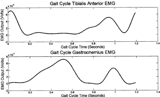
patterns; however, an occasional second peak in the gastocnemius EMG data which does not typically occur in the literature occurred in several of the samples (9).
Gait Cycle Tibialis Anterior EMG
o
0.2 OA 0.6 0. 1 1.2 1.4Gait Cycle Time (Seconds)
~x10'Gait
Cycle Gastrocnemius EMGx 10 W 0 . 0- 2I.-8 2-0 0.2 OA 0.6 0.8 1 1.2 1.4
Gait Cycle Time (Seconds)
Figure 4: Prototypical EMG response for a subject's (top) tibialis anterior and (bottom) gastrocnemius muscles for a gait cycle. EMG output was normalized and overlaid, and the mean response is shown
above.
3.4 Statistics
Student t-tests were performed to determine the likelihood of statistically significant differences in our results.' Various t-tests across appropriate subjects, legs, and loading conditions were performed for the different duration, kinematic, and muscle EMG gait parameters to determine statistical significance. The significance level was set at p = 0.05 for all tests.
4. Results
4.1Duration
Student t-tests between pairs of subjects showed that the differences in mean stride time between subjects' dominant legs in the unloaded condition were statistically significant. Attempts were made to
The author realizes that, in a complete study, Analysis of Variance (ANO VA) should be performed in order to effectively analyze across the multiple subjects and variables. However, due to timing constraints, ANOVA has been deferred to future work.
normalize and pool subject data using a number of scaling factors, but none succeeded. The factors explored were:1) scaling according to subjects' height, 2) scaling according to the inverted pendulum frequency model (i/height), and 3) scaling according to Body Mass Index (BMI), where BMI is defined as:
m
BMI = -
(2)where m is mass of the subject in kilograms and h is subject height in meters.
However, when comparing the mean stride duration between contralateral legs for both loaded and unloaded conditions, the t-tests failed to reject statistical equivalence. In fact, they actually produced high correlation values, with p = 0.9305 as the lowest, and for the rest having p> 0.9704, indicating a high degree of similarity in stride duration times between contralateral legs.
T-tests between loaded and unloaded conditions for both dominant and non-dominant legs yielded significant variation for all subjects, conditions, and legs. While the trends were in opposite directions (Subjects 1 and 3 increased stride duration, while Subject 2 went down), they demonstrated a noteworthy increase in stride duration for subjects (see Table 2).
In order to use the peak ankle plantarflexion to predict toe-off, the temporal consistency of the ankle goniometers had to be ascertained. The mean coefficient of variation (COV) for the timing within each stride of the peak ankle plantarflexion (stance percent) resulted as COV = 0.034, which demonstrated very low variability in the t-test measurement, indicating the ankle goniometer's usefulness as a standard of temporal measurements. T-tests further showed significant differences between both the left and right foot and the loaded and unloaded condition for each subject. However, no trends can be seen in the mean stance time data between the loaded and unloaded condition.
(ps2.79x1035). However, the dominant leg, in the loaded condition, returned much less significant differences, with p-values ranging from 0.0163 to 0.259. T-tests were also performed on the left and right legs and loaded and unloaded conditions and all resulted in statistically significant differences between the left and right legs. However, changes in the mean stance percent appeared similar to changes in stance durations, yielding no clear trends. While the SI did show statistically significant differences between each of the subjects, the mean COV for the SI measurements came to 0.729. In addition, despite the differences, the entire range of the mean SI was restricted from 0.648% to 1.98%, demonstrating a very low absolute change in the SI.
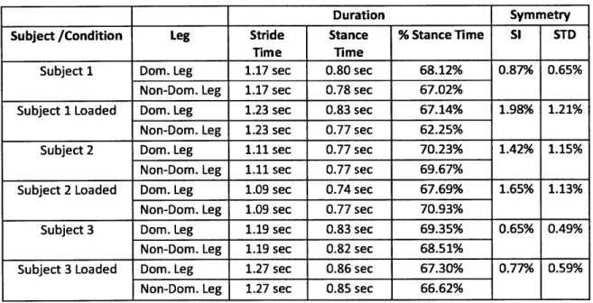
TABLE 2: Mean Duration and Symmetry Parameters
Duration Symmetry
Subject /Condition Leg Stride Stance % Stance Time SI STD
Time Time
Subject 1 Dom. Leg 1.17 sec 0.80 sec 68.12% 0.87% 0.65%
Non-Dom. Leg 1.17 sec 0.78 sec 67.02%
Subject 1 Loaded Dom. Leg 1.23 sec 0.83 sec 67.14% 1.98% 1.21%
Non-Dom. Leg 1.23 sec 0.77 sec 62.25%
Subject 2 Dom. Leg 1.11 sec 0.77 sec 70.23% 1.42% 1.15%
Non-Dom. Leg 1.11 sec 0.77 sec 69.67%
Subject 2 Loaded Dom. Leg 1.09 sec 0.74 sec 67.69% 1.65% 1.13%
Non-Dom. Leg 1.09 sec 0.77 sec 70.93%
Subject 3 Dom. Leg 1.19 sec 0.83 sec 69.35% 0.65% 0.49%
Non-Dom. Leg 1.19 sec 0.82 sec 68.51%
Subject 3 Loaded Dom. Leg 1.27 sec 0.86 sec 67.30% 0.77% 0.59%
Non-Dom. Leg 1.27 sec 0.85 sec 66.62% Finally, the contralateral heel strike
mean values
significant differences between the loaded and unloaded
also came out to have
conditions for both the
percent of stance time (ps0.0071). While the time between heel strikes increased in the loaded
condition for every subject, with some subjects showing significant time increases, the change in
percent of stride fluctuated between subjects, increasing slightly for some while decreasing for
others.
statistically timing and
TABLE3: Contralateral (Loaded/Unloaded) Heel Strike Timing
Subject /Condition Loaded/Unloaded Heel Strikes % of StrideSubject 1 0.59 sec 50.71%
Subject 1 Loaded 0.61 sec 49.20%
Subject 2 0.53 sec 47.86%
Subject 2 Loaded 0.54 sec 49.42%
Subject 3 0.60 sec 50.48%
Subject 3 Loaded 0.64 sec 50.71%
4.2 Kinematics
The timing of the knee and ankle peak angles both produced distributions with surprisingly low variance, as the percent of gait cycle COV's were 0.039 and 0.034, respectively. As mentioned with calculation of stance time, these low COVs indicate the reliability of the goniometer measurements for the temporal aspects of the angle data.
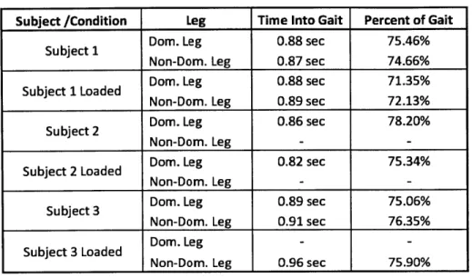
The peak plantarflexion timing of the ankle was already described above (stance time and percent stance time). For the knee peak flexion angle, the time to maximum angle was compared for each loaded and unloaded subject, with a statistically significant difference being observed for each one. Percent of gait cycle till peak knee flexion was also compared across subjects, legs, and loading conditions with a t-test, resulting in statistically significant differences in the mean for each pairing. While the absolute value of the mean peak angle times vary in their response to loading, the timing of the peak knee flexion as a percent of the gait cycle drops noticeably from each non-loaded to loaded condition.
TABLE 4: Peak Knee Flexion Timing
4.3 EMG Activity
Unlike the goniometer output, the COV values for the mean EMG per stride demonstrated a notable amount of variance, with an average COV = 0.30 for the tibialis anterior and an average COV =
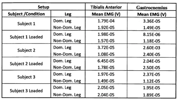
0.32 for the gastrocnemius. Both the tibialis anterior and gastrocnemius were analyzed with t-tests between the loaded and unloaded conditions for each subject and leg. Significant statistical differences between each case were determined (p 7.2x10⁻⁷), except for Subject 2's non-dominant foot (p = 0.34). This appears to be an unexplained anomaly but further work is required to establish that speculation. While the mean outputs all vary significantly, no clear trend can be seen in the data (see Table 5).
Subject /Condition Leg Time Into Gait Percent of Gait Subject 1 Dom. Leg 0.88 sec 75.46%
Non-Dom. Leg 0.87 sec 74.66%
Subject 1 Loaded Dom. Leg 0.88 sec 71.35% Non-Dom. Leg 0.89 sec 72.13%
Subject 2 Dom. Leg 0.86 sec 78.20%
Non-Dom. Leg -
-Subject 2 Loaded Dom. Leg 0.82 sec 75.34%
Non-Dom. Leg -
-Subject 3 Dom. Leg 0.89 sec 75.06%
Non-Dom. Leg 0.91 sec 76.35%
Subject 3 Loaded Dom. Leg -
TABLE 5: Mean EMG Output per Stride
Setup Tibialis Anterior Gastrocnemius Subject /Condition Leg Mean EMG (V) Mean EMG (V)
Subject 1 Dom. Leg 1.79E-04 3.36E-05
Non-Dom. Leg 1.92E-05 1.49E-05 Subject 1 Loaded Dom. Leg 1.98E-05 8.15E-06
Non-Dom. Leg 1.57E-05 1.18E-05
Subject 2 Dom. Leg 3.72E-05 2.60E-03
Non-Dom. Leg 1.08E-05 2.40E-05 Subject 2 Loaded Dom. Leg 6.45E-05 2.04E-05 Non-Dom. Leg 1.78E-05 2.50E-05
Subject 3 Dom. Leg 1.97E-05 2.37E-05
Non-Dom. Leg 1.49E-05 1.12E-05 Subject 3 Loaded Dom. Leg 2.05E-05 1.95E-05
Non-Dom. Leg 2.04E-05 1.89E-05
5.
Conclusion
The results presented above demonstrated a clear change in the biomechanical response due to the loading of the system, especially in the gait duration data. In particular, the clear changes in stride durations, especially in Subjects 1 and 3, demonstrated the effects of the loading. While the results for Subject 2 differed for stride duration time, lengthening the duration instead of shortening it, a range of variables, such as height or sex, may account for this variation, and further study is required to ascertain the cause.
In contrast, the equivalence of duration for contralateral strides in both the loaded and unloaded condition points to a regulating mechanism to adjust one leg to the rhythm of the other. Clearly the ground's physical reaction forces play some role in keeping the mean stride times equal, but there also appears to be a neurological control system governing the behavior. In addition, the appearance of similarities in percent stance of the loaded leg between subjects may indicate an attempt by the neural controller to regulate aspects of the gait cycle, but this speculation remains unproven.
Moreover, exploration of the SI did not reveal any truly important differences under loading. While it is true that the SI increased in the loaded case for all subjects, the large COV of the SI and the
inherently low mean SI values made it difficult to claim a truly notable increase in asymmetry. However, the analysis of contralateral heel strikes showed a consistently small change in percent phase shift. This minimization of change is indicative of a mechanism that adjusts the relative timing of steps to keep walking cadences out of phase despite asymmetric lower limb loading.
While the data presented by kinematic and EMG analysis provided limited conclusions, one important note was the propensity for the peak knee flexion to shift to earlier in the gait cycle when under loading. This shift could correlate with the reduction in nonparetic peak knee flexion noted by Khanna et al. (7). An earlier peak in the knee cycle, rather than indicating a shift in the timing of the knee flexion, could also indicate a shortened activation of knee flexors, which would lead to a peak lower angle. In the current experiment, the subject's healthy range of motion would have allowed them to display the shortened knee flexion in both legs rather than just the nonparetic limb, as happened with Khanna et al.'s subjects.
In summary, it is clear that, regardless of the other biomechanical gait parameters, the body adjusts itself to minimize any temporal asymmetry it may experience under asymmetric loading.
6. Future Work
While this preliminary study's results reveal several significant trends, most notably the temporal symmetry and control of the lower limb locomotion under loading, many further analysis techniques and experimental adjustments could be made to yield valuable further data.
One important change that will be crucial to pursue in future work is the change from multiple t-tests to ANOVA. ANOVA will prove more accurate than multiple t-t-tests in analyzing the data, as it will be able to better incorporate multiple populations. It will also be able to incorporate and deal with the multiple factors (loading, left and right leg) in a multiple factor ANOVA test. Finally, as an F-test ANOVA has the ability to differentiate between assignable and random causes between populations, an important factor in human biomechanics data.
In addition, while the temporal data obtained in the current work is a start, the ability to measure knee and ankle angles is crucial to a better understanding of asymmetrically loaded walking. In order to do so, a more thorough knowledge of the current goniometers or new goniometers must be obtained. In particular, confirmation of Khanna et al.'s reported change in the nonparetic peak knee flexion and paretic knee dorsiflexion would be beneficial (7). This information, combined with goniometer confirmation of the temporal location of the beginning of knee flexion, would demonstrate whether or not the shift in knee flexion timing observed in the current experiment is indicative of an overall phase shift in knee flexion, or merely a shortening of the flexor muscle output. It would also reveal a great deal about the underlying strategies used to adjust to the heavier loads. In addition, a more accurate angular analysis of flexion and extension would help to confirm other limb trajectories affected by asymmetric loading.
Finally, this pilot test explored quadriceps and hamstring EMG placement and setup. The author recommends that further tests should build upon this paper's work, especially ensuring secure attachment of the sensors and routing of the cables, as later tests with a more refined system setup showed better results than earlier tests. The quadriceps placement should also be considered, as the results for the current experiment often led to frequencies indicative of an artifact. The information from these EMG sensors would do a great deal to illuminate the control strategy used to regulate lower limb walking in response to the loading-the changes or lack thereof in kinematics should be equally correlated with responses from the EMG output. Not only would EMG data be helpful for magnitude comparisons, but temporal analysis of muscle activation would illuminate certain timing aspects of the control.
7. Appendix
Appendix A
-
Goniometer Calibration Methods
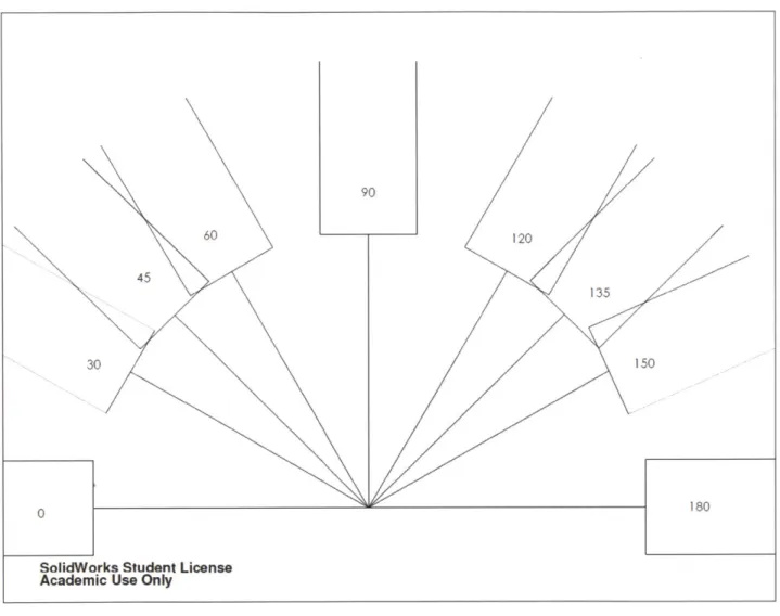
In order to calibrate the goniometers, a degree calibration sheet was made from SolidWorks* 2011 with angles from 30-180 degrees. The goniometer was positioned at each of the angles four times, and the voltage output from the goniometer was recorded through the calibration test. The outputs were recorded through the DelsysMyomonitor* system.
Figure
5:
The goniometers were calibrated by moving the
goniometers along the angle pattern sheet.
Both directions of flexion on the goniometer were calibrated separately. The voltage
output results were fit in MATLAB using the POLYFIT function. Unfortunately, the
goniometers became unreliable near the 30 and 180 degrees limits, as well as being imprecise
throughout the entire goniometer range.
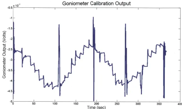
Goniometer Calibration Output
200
Time (sec)
Figure 6: Sample goniometer calibration voltage output.
goniometer
was
traced
back
and
forth
on
SolidWorkscalibration sheet twice to obtain the calibration
points.
The
the
data
Figure 7: The goniometer. The positioning of the ID numbers
(lower left hand block) was used as the reference for the direction
of the goniometer. The double sided mounting tape can be seen on
the upper right block.
Appendix B- Usable Data
TABLE
6:
Usable Data Subject 1Unloaded Non- Loaded
Non-Unloaded Dom Dom Loaded Dom Dom
Knee Gonio Good Good Good Good
Ankle Gonio Good "" Good "" Good " Good
Quad EMG Bad Bad Bad Bad
Ham EMG Bad Good "" Good "" Good TA EMG Good "" Good "" Good "" Good Gastro EMG Bad Good "" Good "" Good
Heel Switch Good Good Good Good
Subject 2
Unloaded Non- Loaded Loaded
Non-Unloaded Dom Dom Dom*** Dom***
Knee Gonio Good Bad Good Bad
Ankle Gonio Good "" Good Good Good
Quad EMG Bad Bad Bad Bad
Ham EMG Bad Bad Bad Bad
TA EMG Good "" Good Bad Good
Gastro EMG Bad Good Bad Good
Heel Switch Good** Good Good** Good
Subject 3
Unloaded Non- Loaded
Non-Unloaded Dom Dom Loaded Dom Dom
Knee Gonio Good Good Bad Good ""
Ankle Gonio Good "" Good Good Good
Quad EMG Bad Good "" Good Bad
Ham EMG Good "" Good "" Bad Bad
TA EMG Good Good "" Good Good
Gastro EMG Good Good "" Good Good
Heel Switch Good Good Good Good
Good Indicates good reading Bad Indicates bad reading
Good " Indicates needed to remove random spikes
**Subject 2's dominant leg has weird peaks in the heel strike data, causing large deviations in spread
Appendix C- Sample Code for Data Processing
Sample Code For Subject I in the Unloaded Trial
dat = subldat;
subnum = 'subi';
enddat = 600000;
halfdat = 300000;
%Removing spikes from data
%optional - dedends on data***** %dom ankle remove = dat(:,3); remove(remove < -. 0038) = -. 00344; dat(:,3) = remove; %non-dom ankle remove = dat(:,10); remove(remove < -. 00406) = -. 0038; dat(:,10) = remove; %dom TA remove = dat(:,6); remove(remove > .0006 dat(:,6) = remove; %non-dom Ham remove = dat(:,12); remove(remove > .0003 dat(:,12) = remove; %non-dom TA remove = dat (:,13); remove(remove > .0004 dat(:,13) = remove; %non-dom Gastro remove = dat(:,14); remove(remove > .0002 dat(:,14) = remove;
& remove<-.0008 ) = mean(remove);
& remove<-.0003 ) = mean(remove);
& remove<-.0005 ) = mean(remove);
& remove<-.0004 ) = mean(remove);
%Goniometers - volts to degrees. Infor comes from calibratoin script %check to insure correct orientation of goniometer
figure(1); t= dat(:,1); %Knee Dominant. subplot (2,2,1); w = dat(:,2); dat(:,2) = 1.0e+008*(4.020751325121656*w.^3 -0.007183393503045*w.^2 +
-plot(t(300001:310000), 1.0e+008 *(4.020751325121656*w(300001:310000) A3 -0.007183393503045*w(300001:310000).^2 + 0.000431669254195*w(300001:310000).^1 + 0.000000968179196)); %Ankle Dom. subplot(2,2,2); x = dat(:,3); dat(:,3) = 1.0e+005 *(-6.796266001448857*x.^2 + 0.463210635990114*x+ 0.002134919571317); plot(t(300001:310000), 1.0e+005 *(-6.796266001448857*x(300001:310000).^2 + 0.463210635990114*x(300001:310000)+ 0.002134919571317)); %Knee Alt. subplot(2,2,3); z = dat(:,9);
dat(:,9) = 1.Oe+010 *( -1.636709553700273*z.A3 -0.009902638748577*z.A2
-0.000026756956310*z -0.000000015382608);
plot(t(300001:310000), 1.0e+010 *( -1.636709553700273*z(300001:310000).A3
-0.009902638748577*z(300001:310000).^2 -0.000026756956310*z(300001:310000)
-0.000000015382608));
%Ankle Alt.
subplot(2,2,4); y = dat(:,10);
dat(:,10) = 1.0e+009 *(-3.257033868770031*y.A3 -0.042575152240692*y.A2
-0.000121964934110*y +0.000000083224399);
plot(t(300001:310000), 1.0e+009 *(-3.257033868770031*y(300001:310000).^3
-0.042575152 24069 2*y(3 0 0 0 01:310000).^2 -0.000121 9 6 4 9 3 4110*y( 300001: 310000)
+0.000000083224399));
%Legl
%Calculating average stride time %Locating footswitch data
%locating peaks on footswitch
%unloaded - we want just the values from 300sec onward, really. [maga,loca] = findpeaks(dat(:,8), 'MINPEAKDISTANCE', 1000);
mag = maga(2:(length(maga))); %check
if need this for peak heel before heel strike loc = loca(2:(length(loca)));
%find heel strike lcations - it assumes set maginitude of for %start of heel strike - may change
relheelswitch = dat(1:enddat,8); peakbeginnings = zeros(size(loc)); pbheight = zeros(size(loc)); fori=l:length(loc) height = mag(i); j=0; while height > .00031
%%%%%%changes per subject
j=j+1;
end
peak-beginnings(i)=loc(i)-j;
pb-height(i) = dat(peak-beginnings(i), 8); end
%calculate the number of strides numstrides = length(mag)-1;
%stride time - actual times and location of times stridetime = diff(dat(loc,1)); stridetimeloc = diff(loc); meanstridetimeloc = mean(stridetimeloc); meanstridetime = mean(stridetime); medianstridetimeloc = median(stridetimeloc); medianstridetime = median(stridetime);
usestridetime = round(meanstridetimeloc); %notice that this is the data index length of stride time, not the actual stride time itself, which will be off by about .0022 per stride length
%heel strike - this is the location of the time index, not the time- we care about
%the location to call for overlay later heelstridet = diff(peak-beginnings); mean(heelstridet); halfheelloc = find(dat(peak-beginnings,1)>300,1); halfheeltime peak-beginnings(halfheelloc); stridetimebeg = stridetime(1:(halfheelloc)); meanstridetimebeg = mean(stridetimebeg); stridetimeend = stridetime(halfheelloc:length(stridetime)); meanstridetimeend = mean(stridetimeend);
%plot - distribution of time figure(2)
%whole thing
histobox = (round(min(stridetime))):.001:(round(max(stridetime))+.6); %%%check borders of histogram per subject
subplot (1,3,1)
hist(stridetime, histobox);
%first half
histobox = (round(min(stridetime))):.001:(round(max(stridetime))+.6);
%%%check borders of histogram per subject
subplot(1,3, 2)
hist(stridetime(1:(halfheelloc-1)), histobox);
title([subnum'legl_''_distribution of stridetime'])
histobox = (round(min(stridetime))):.001:(round(max(stridetime))+.6); %%%check borders of histogram per subject
subplot(1,3,3) hist(stridetime(halfheelloc:length(stridetime)), histobox); %plot stridetime figure(3) %full subplot(1,3,1); t = 1:length(stridetime); plot(t, stridetime, 'b'); %beg subplot(1,3,2); t = 1:(halfheelloc-1); stridetimebeg = stridetime(1:(halfheelloc-1)); plot(t, stridetimebeg); title([subnum'_legl_''_stridetime']) %end subplot (1, 3, 3); t = (halfheelloc):length(stridetime); stridetimeend = stridetime((halfheelloc):length(stridetime)); plot(t,stridetimeend);
%plot heelstridetime and heelstrikes figure(4)
subplot (2, 1, 1);
title([subnum'_legl_''_heelstrike'])
plot(heelstridet)
subplot(2,1,2);
plot( dat(1:length(dat),1), dat(1:length(dat),8), 'b',
dat ((peak-beginnings (1:length (pbheight)) ), 1),
pbheight(1: (length(pb-height))), 'r*')
%rectify and filter EMG data %unloaded
fori = 4:7;
dat(:,i) Butter4_LowPassFilter(abs(dat(:,i)-mean(dat(:,i))), 1000, 5); end
%overlay
%average data set for subject
%prep matrix for subject average data
avealldata = zeros(usestridetime,15);
avealldataend = zeros(usestridetime,15); %first column is time
avealldata(:,1) = dat(1:usestridetime, 1); avealldatabeg(:,1) = dat(1:usestridetime, 1); avealldataend(:,1) = dat(1:usestridetime, 1);
for j = 2:8;
%single vector for subject %prep matrix for vector
sumivectordata = zeros((numstrides),usestridetime);
%call data - except last one because of end effect of
%resample
% first stride callstrideextra =
dat(((peak-beginnings(1))):((peak9beginnings(1))+2*heelstridet(1) - 1),j); callstridenorm = resample(callstrideextra, (usestridetime-1),
(heelstridet(numstrides)-1)); callstrideuse = callstridenorm(1:(usestridetime)); sumlvectordata(1,:) = callstrideuse'; fori = 2:(numstrides-1) callstrideextra = dat(((peak-beginnings(i))+ (1 -heelstridet(i))):((peak_beginnings(i))+2*heelstridet(i) - 1),j); size(callstrideextra);
callstridenorm = resample(callstrideextra, (usestridetime-1), (heelstridet(i)-1)); size(callstridenorm); callstrideuse = callstridenorm((usestridetime):(2*usestridetime-1)); size(callstrideuse'); size(sumnvectordata); sumlvectordata(i,:) = callstrideuse'; end % last stride callstrideextra = dat(((peakbeginnings(numstrides))+ (1 -heelstridet(numstrides))):length(dat),j);
callstridenorm = resample(callstrideextra, (usestridetime-1), (heelstridet(numstrides)-1));
callstrideuse = callstridenorm((usestridetime):(2*usestridetime-1)); sumivectordata(numstrides,:) = callstrideuse';
%split to first half and last half
sumivectordatabeg = sumlvectordata(1:(halfheelloc-1),:); sumlvectordataend = sumlvectordata(halfheelloc:numstrides,:);
%turn into one average stride
aveallstride = sum(sumlvectordata)/numstrides;
aveallstridebeg = sum(sumlvectordatabeg)/(halfheelloc-1);
if j == 2 %%%these
depend on the front back orientation of the goniometer*******
allkneenorm = sumvectordata;
aveallstride -aveallstride +max(aveallstride);
aveallstridebeg = -aveallstridebeg + max(aveallstridebeg);
aveallstrideend = -aveallstrideend + max(aveallstrideend);
end
%correct for angle on ankle
if j == 3 %%%these
depend on the front back orientation of the goniometer*******
allanklenorm = sumvectordata;
% allanklenormbeg = sumlvectordatabeg;
% allanklenormend = sumlvectordataend;
aveallstride = -aveallstride + aveallstride(1);
aveallstridebeg = -aveallstridebeg + aveallstridebeg(1); aveallstrideend = -aveallstrideend + aveallstrideend(1);
end if j == 6; allta = sumivectordata; meantavals = mean(allta, 2); meantagait = mean(allta); end if j == 7; allgastroc = sumivectordata; meangastrocvals = mean(allgastroc, 2); meangastrocgait = mean(allgastroc); end figure (j+3); subplot(2, 1,1); title([subnum'_legl_']) plot(dat((1:usestridetime), 1), aveallstride,'b', dat((l:usestridetime), 1), aveallstridebeg,'g',dat((1:usestridetime), 1),
aveallstrideend, 'c', dat((1: (usestridetime)),1),
dat(((halfheeltime):(halfheeltime+ usestridetime-1)),j),'r'); subplot (2,1,2); holdon for n = 1:(halfheelloc-1); plot(1:usestridetime, sumlvectordatabeg(n,:),'b'); end for n = (halfheelloc:numstrides)-halfheelloc+1; plot(1:usestridetime, sumlvectordataend(n,:),'r'); end holdoff
%add to all vectors
avealldatabeg(:,j) = aveallstridebeg; avealldataend(:, j) = aveallstrideend; end figure(100) holdon for j = 2:3 plot(avealldata(:,1), avealldata(:,j),'b') end plot(avealldata(:,1), avealldata(:,4)*2000000,'r') plot(avealldata(:,1), avealldata(:,5)*3000000,'y') plot(avealldata(:,1), avealldata(:,6)*1000000,'g') plot(avealldata(:,1), avealldata(:,7)*1000000,'cI) plot(avealldata(:,1), avealldata(:,8)*100000,'k') title([subnumI legl_''_overlay all'])
holdoff
%Find toe-off point
[maganknorm, locanknorm] = max(allanklenorm(:,500:900), [],2); %double check the bound numbers for each stride - should be similar.***********
locanknorm = locanknorm+500; %re-add the stride location maganknorm = maganknorm'; locanknorm = locanknorm'; % locanknormbeg = locanknorm(1:(halfheelloc-1)); % locanknormend = locanknorm(halfheelloc:length(locanknorm)); figure(12) subplot (1, 2, 1); title([subnum'_legl_''_Loe-strike check']) plot(1:numstrides,locanknorm); histoboxtoe = (round(min(locanknorm)-1)):(round(max(locanknorm))+1); %******each histobox will be different
subplot (1,2,2);
hist(locanknorm, histoboxtoe);
%Since small variance in location of ankle output.
%Take raw data and overlay it, un-normalized.
%prep matrix for vector
sumlankledata = zeros(numstrides,usestridetime);
fori = 1:(numstrides);
sumlankledata(i,:) =
dat(((peak-beginnings(i)):(peak-beginnings(i)+usestridetime-1)),3)';
end
[magank, locank] = max(sumlankledata(:,600:900), [], 2);
%***sub 1 calls the wrong data twice, because of the second spike being
higher.
magank = magank'; locank = locank+600; locank = locank';
%locank are the locations of the toeoffs (locank(i)+300000)
fori = 1:numstrides; stancetimes(i) = dat((peakbeginnings(i)+locank(i)),1)-dat((peak-beginnings(i)), 1); end stancetimesbeg = stancetimes(1:(halfheelloc-1)); stancetimesend = stancetimes(halfheelloc:numstrides); figure(50) subplot (1, 2, 1);
title( [subnum'_legl' '_stancetimes all '])
plot(1:length(stancetimes), stancetimes);
histoboxtoe = (round(min(stancetimes))-.5):.001:(round(max(stancetimes))-.1);
%******each histobox will be different
subplot (1,2,2);
hist(stancetimes, histoboxtoe);
figure(51)
title( [subnum'_legl_'' begendstancetimes'])
histboxbeg = (round(min(stancetimesbeg))-.5) :.001:(round(max(stancetimesbeg))-.1); histboxend = (round(min(stancetimesend) )-.5) :.001:(round(max(stancetimesend))-.1); subplot (1,2,1); hist(stancetimesbeg, histboxbeg); subplot (1,2,2); hist(stancetimesend, histboxend); figure(52) allkneenormplot = zeros(size(sumlvectordata)); allanklenormplot = zeros(size(sumlvectordata)); fori = 1:numstrides;
allkneenormplot(i,:) = - allkneenorm(i,:) + max(allkneenorm(i,:)); allanklenormplot(i,:) = -allanklenorm(i,:) + (allanklenorm(i,1)); end
plot (allanklenormplot', allkneenormplot');
title( [subnum'_legl' '_ankleknee'])
%Take raw data and overlay it, un-normalized.
%prep matrix for vector
sum1kneedata = zeros(numstrides,usestridetime); fori = 1:(numstrides);
sumlkneedata (i,:) =
dat(((peak-beginnings(i)):(peak-beginnings(i)+usestridetime-1)),2)';
end
[magknee, locknee] = max(abs(sumlkneedata(:,600:1100)), [], 2);
%***sub 1 calls the wrong data twice, because of the second spike being
higher.
magknee = magknee'; locknee = locknee+600; locknee = locknee';
%locknee are the locations of Lhe Loeoffs (locknee(i)+300000)
kneeflextimes = zeros(numstrides,1); fori = 1:numstrides; kneeflextimes(i) = dat((peakbeginnings(i)+locknee(i)),1)-dat((peak-beginnings(i)), 1); end %non-dominant leg********************************************************* %Calculating average stride time
%Locating footswitch data %locating peaks on footswitch
%unloaded - we want just the values from 300sec onward, really. [mag2,loc2] = findpeaks(dat(:,15), 'MINPEAKDISTANCE', 1000);
%find heel strike lcations - it assumes set maginitude of for %start of heel strike - may change
relheelswitch2 = dat(1:enddat,15);
peak beginnings2 = zeros(size(loc2)); pb-height2 = zeros(size(loc2)); fori=1:length(loc2)
height = mag2(i); j=0;
while height > .00029 %%%%%%changes per subject j=j+l; height = relheelswitch2(loc2(i)-j); end peakbeginnings2(i)=loc2(i)-j; pb-height2(i) = dat(peak.beginnings2(i), 15); end
%calculate the number of strides numstrides2 = length(mag2)-1;
%stride time - actual times and location of times stridetime2 = diff(dat(loc2,1)); stridetimeloc2 = diff(loc2); meanstridetimeloc2 = mean(stridetimeloc2); meanstridetime2 = mean(stridetime2); medianstridetimeloc2 = median(stridetimeloc2); medianstridetime2 = median(stridetime2);
usestridetime2 = round(meanstridetimeloc2); %notice data index length of stride time, not the actual stride time will be off by about .0022 per stride length
that this is the
itself, which
%heel strike - this is the location of the time index, not the time- we care
about
%the location to call for overlay later
heelstridet2 = diff(peak-beginnings2); mean(heelstridet2);
halfheeltime2 = peakbeginnings2(halfheelloc2);
stridetimebeg2 = stridetime2(1:(halfheelloc2));
meanstridetimebeg2 = mean(stridetimebeg2);
stridetimeend2 = stridetime2(halfheelloc2:length(stridetime2));
meanstridetimeend2 = mean(stridetimeend2);
%plot - distribution of stridetime
figure(13)
%whole thing
histobox2
(round(min(stridetime2))):.001:(round(max(stridetime2))+.6); %%%check borders of histogram per subject
subplot(1,3,1)
hist(stridetime2, histobox2);
%first half
histobox2 =
(round(min(stridetime2))):.001:(round(max(stridetime2))+.6); %%%check borders of histogram per subject
subplot(1, 3,2)
hist(stridetime2(1:(halfheelloc2-1)), histobox2);
title( [subnum'_leg2' 'distr. of stridetime'])
%second half
histobox2 =
(round(min(stridetime2))):.001:(round(max(stridetime2))+.6); %%%check borders of histogram per subject
subplot (1,3,3) hist(stridetime2(halfheelloc2:length(stridetime2)), histobox2); %plot stridetime figure(14) %full subplot(1,3,1); t2 = 1:length(stridetime2); plot(t2, stridetime2, 'b'); %beg subplot (1, 3, 2); t2 = 1:(halfheelloc2-1); stridetimebeg2 = stridetime2(1:(halfheelloc2-1)); plot(t2, stridetimebeg2); title([subnum'_leg2_''_stridetimes']) %end subplot(1,3,3); t2 = (halfheelloc2):length(stridetime2); stridetimeend2 = stridetime2((halfheelloc2):length(stridetime2)); plot(t2,stridetimeend2);
%plot heelstridetime and heelstrikes figure (15)
subplot (2, 1, 1)
plot(heelstridet2)
title([subnumlieg2_''_heelstridet and strikes'])
subplot (2, 1, 2) ;
plot( dat(1:length(dat) ,1), dat(1:length(dat),15), 'b', dat( (peak-beginnings2 (1:length(pbheight2) ) ) ,1),
pb_height2 (1: (length(pbheight2))), 'r*')
%rectify and filter EMG data %unloaded
fori = 11:14;
dat(:,i) = Butter4_LowPassFilter(abs(dat(:,i)-mean(dat(:,i))), 1000, 5); end
%overlay
%average data set for subject
%prep matrix for subject average data
for j = 9:15;
%single.vector for subject %prep matrix for vector
sumlvectordata2 = zeros( (numstrides2) ,usestridetime2) ;
%call data - except last one because of end effect of %resample
% first stride
callstrideextra2 =
dat(((peak-beginnings2(1))) : ((peakbeginnings2(1))+2*heelstridet2(1) - 1),j);
callstridenorm2 = resample (callstrideextra2,
(usestridetime2-1), (heelstridet2(numstrides2)-1));
callstrideuse2 = callstridenorm2 (1: (usestridetime2)); sumlvectordata2(1,:) = callstrideuse2';
fori = 2:(numstrides2-1)
callstrideextra2 = dat( ( (peak_beginnings2 (i) ) + (1
-heelstridet2(i))):((peak_beginnings2(i))+2*heelstridet2(i) - 1),j);
size(callstrideextra2);
callstridenorm2 = resample (callstrideextra2, (usestridetime2-1), (heelstridet2(i)-1)); size(callstridenorm2); callstrideuse2 = callstridenorm2((usestridetime2):(2*usestridetime2-1)); size(callstrideuse2'); size(sumlvectordata2); sum1vectordata2(i,:) = callstrideuse2'; end
callstrideextra2 = dat(((peak_beginnings2(numstrides2))+ (1
-heelstridet2(numstrides2))):length(dat),j);
callstridenorm2 = resample(callstrideextra2, (usestridetime2-1), (heelstridet2(numstrides2)-1));
callstrideuse2 =
callstridenorm2((usestridetime2):(2*usestridetime2-1));
sumlvectordata2(numstrides2,:) = callstrideuse2';
%split to first half and last half
sumlvectordatabeg2 = sumlvectordata2(1:(halfheelloc2-1),:);
sumlvectordataend2 =
sumvectordata2(halfheelloc2:numstrides2,:);
%turn into one average stride
aveallstride2 = sum(sumlvectordata2)/numstrides2;
aveallstridebeg2 = sum(sumlvectordatabeg2)/(halfheelloc2-1);
aveallstrideend2 =
sum(sumlvectordataend2)/(numstrides2-halfheelloc2+1);
%correct for angle on knee
if j == 9 %%%these
depend on the front back orientation of the goniometer*******
allkneenorm2 = sumlvectordata2;
aveallstride2 = -aveallstride2 + max(aveallstride2);
aveallstridebeg2 = -aveallstridebeg2 +
max(aveallstridebeg2);
aveallstrideend2 = -aveallstrideend2 +
max(aveallstrideend2);
end
%correct for angle on ankle if j == 10
allanklenorm2 = sumlvectordata2;
% allanklenormbeg = sumivectordatabeg;
% allanklenormend = sumlvectordataend;
aveallstride2 = -aveallstride2 + aveallstride2(1);
aveallstridebeg2 = -aveallstridebeg2 + aveallstridebeg2 (1); aveallstrideend2 = -aveallstrideend2 + aveallstrideend2(1); end if j == 13; allta2 = sumlvectordata2; meantavals2 = mean(allta2, 2); meantagait2 = mean(allta2); end if j == 14; allgastroc2 = sumlvectordata2;
meangastrocvals2 = mean(allgastroc2, 2); meangastrocgait2 = mean(allgastroc2); end figure (j+7); subplot (2, 1, 1) ; plot(dat((1:usestridetime2), 1), aveallstride2,'b', dat((l:usestridetime2), 1), avealistridebeg2,'g',dat((1:usestridetime2), 1), aveallstrideend2,'c', dat((1:(usestridetime2)),1), dat(((halfheeltime2):(halfheeltime2+ usestridetime2-1)),j),'r'); subplot(2,1,2); holdon for n = 1:(halfheelloc2-1); plot(1:usestridetime2, sum1vectordatabeg2(n,:),'b'); end for n = (halfheelloc2:numstrides2)-halfheelloc2+1; plot(1:usestridetime2, sumlvectordataend2(n,:),'r'); end holdoff
%add to all vectors
avealldata(:,j) = aveallstride2; avealldatabeg(:,j) = aveallstridebeg2; avealldataend(:, j) = aveallstrideend2; end figure (23) holdon for j = 9:10 plot(avealldata(:,1), avealldata(:,j),'b') end plot(avealldata(:,1), avealldata(:,11)*200 plot(avealldata(:,1), avealldata(:,12)*300 plot(avealldata(:,1), avealldata(:,13)*100 plot(avealldata(:,1), avealldata(:,14)*100 plot(avealldata(:,1), avealldata(:,15)*100 title([subnum'-leg2_''_overlay all ']) holdoff 0000, 'r' 0000, 'y' 0000,'g' 0000,'c' 000, 'k')
%Find toe-off point
[maganknorm2, locanknorm2l = max(allanklenorm2(:,500:850), [],2); %double check the bound numbers for each stride - should be similar.*********** locanknorm2 = locanknorm2+500; maganknorm2 = maganknorm2'; locanknorm2 = locanknorm2'; % locanknormbeg = locanknorm(1:(halfheelloc-1)); % locanknormend = locanknorm(halfheelloc:length(locanknorm)); figure(24) subplot (1, 2, 1);
title([subnum'_leg2_''_test ankle loc'])
histoboxtoe2 = (round(min(locanknorm2)-1)):(round(max(locanknorm2))+1); %******each histobox will be different
subplot (1,2,2);
hist(locanknorm2, histoboxtoe2);
%Since small variace in location of ankle output. %Take raw data and overlay it, un-normalized. %prep matrix for vector
sumlankledata2 = zeros(numstrides2,usestridetime2);
fori = 1:(numstrides2); sumlankledata2(i,:) =
dat(((peak-beginnings2(i)):(peak_beginnings2(i)+usestridetime2-1)),10)';
end
[magank2, locank2] = max(sumlankledata2(:,600:850), [], 2); %***sub 1 calls the wrong data twice, because of the second spike being higher.
magank2 = magank2'; locank2 = locank2+600; locank2 = locank2';
%locank are the locations of the toeoffs (locank(i)+300000) %need to find stance time - have toe-off and heel-strike.
stancetimes2 = zeros(numstrides2,1); fori = 1:numstrides2; stancetimes2(i) = dat((peak-beginnings2(i)+locank2(i)),1)-dat((peakbeginnings2(i)), 1); end stancetimesbeg2 = stancetimes2(1:(halfheelloc2-1)); stancetimesend2 = stancetimes2(halfheelloc2:numstrides2); figure(60) subplot (1, 2, 1); plot(1:length(stancetimes2), stancetimes2);
title( [subnum'_leg2' '_stancetimes all'])
histoboxtoe2 =
(round(min(stancetimes2))-.3):.001:(round(max(stancetimes2))-.1); %******each histobox will be different
subplot(1,2,2); hist(stancetimes2, histoboxtoe2); figure(61) histboxbeg2 = (round(min(stancetimesbeg2))-.3):.001:(round(max(stancetimesbeg2))-.1); histboxend2 = (round(min(stancetimesend2))-.3):.001:(round(max(stancetimesend2))-.1); subplot (1,2,1); hist(stancetimesbeg2, histboxbeg2);
title( [subnum'_leg2_ 'begend stance times'])
subplot (1, 2, 2) ;
figure (62)
allkneenormplot2 = zeros(size(sumlvectordata2)); allanklenormplot2 = zeros(size(sumlvectordata2));
fori = 1:numstrides2;
allkneenormplot2(i,:) = - allkneenorm2(i,:) + max(allkneenorm2(i,:)); allanklenormplot2(i,:) = -allanklenorm2(i,:) + (allanklenorm2(i,1)); end
plot(allanklenormplot2', allkneenormplot2'); title([subnum'_leg2_'' ankleknee'])
%Take raw data and overlay it, un-normalized - knee data. %prep matrix for vector
sumlkneedata2 = zeros(numstrides2,usestridetime2); fori = 1:(numstrides2); sumlkneedata2(i,:) = dat(((peak-beginnings2(i)):(peakbeginnings2(i)+usestridetime2-1)),9)'; end holdoff
[magknee2, locknee2] = min(abs(sumlkneedata2(:,600:1100)), [], 2); %***sub 1 calls the wrong data twice, because of the second
spike being higher.
magknee2 = magknee2'; locknee2 = locknee2+600; locknee2 = locknee2';
%locknee are the locations of the max knee flexion(locknee (i)+300000) %need to find stance time - have toe-off and heel-strike.
kneeflextimes2 = zeros(numstrides2,1); fori = 1:numstrides2;
kneeflextimes2(i) = dat((peak-beginnings2(i)+locknee2(i)),1)-dat((peakbeginnings2(i)), 1);
end
%compute important data
meanstancetimes = mean(stancetimes); meanstancetimesbeg = mean(stancetimesbeg); meanstancetimesend = mean(stancetimesend); meanstancetimes2 = mean(stancetimes2); meanstancetimesbeg2 = mean(stancetimesbeg2); meanstancetimesend2 = mean(stancetimesend2); meanall = mean(avealldata); highpeakall = max(avealldata); lowpeakall = min(avealldata);