Condition assessment of buried pipes using hierarchical evidential reasoning model

Publisher’s version / Version de l'éditeur:

Journal of Computing in Civil Engineering, 22, March/April 2, pp. 114-122, 2008-03-01

READ THESE TERMS AND CONDITIONS CAREFULLY BEFORE USING THIS WEBSITE.

https://nrc-publications.canada.ca/eng/copyright

Vous avez des questions? Nous pouvons vous aider. Pour communiquer directement avec un auteur, consultez la première page de la revue dans laquelle son article a été publié afin de trouver ses coordonnées. Si vous n’arrivez pas à les repérer, communiquez avec nous à PublicationsArchive-ArchivesPublications@nrc-cnrc.gc.ca.

Questions? Contact the NRC Publications Archive team at

PublicationsArchive-ArchivesPublications@nrc-cnrc.gc.ca. If you wish to email the authors directly, please see the first page of the publication for their contact information.

NRC Publications Archive

Archives des publications du CNRC

This publication could be one of several versions: author’s original, accepted manuscript or the publisher’s version. / La version de cette publication peut être l’une des suivantes : la version prépublication de l’auteur, la version acceptée du manuscrit ou la version de l’éditeur.

For the publisher’s version, please access the DOI link below./ Pour consulter la version de l’éditeur, utilisez le lien DOI ci-dessous.

https://doi.org/10.1061/(ASCE)0887-3801(2008)22:2(114)

Access and use of this website and the material on it are subject to the Terms and Conditions set forth at Condition assessment of buried pipes using hierarchical evidential reasoning model

Hua, B.; Sadiq, R.; Najjaran, H.; Rajani, B. B.

https://publications-cnrc.canada.ca/fra/droits

L’accès à ce site Web et l’utilisation de son contenu sont assujettis aux conditions présentées dans le site LISEZ CES CONDITIONS ATTENTIVEMENT AVANT D’UTILISER CE SITE WEB.

NRC Publications Record / Notice d'Archives des publications de CNRC:

https://nrc-publications.canada.ca/eng/view/object/?id=3673289f-e291-4313-98db-52597a07480a https://publications-cnrc.canada.ca/fra/voir/objet/?id=3673289f-e291-4313-98db-52597a07480a

http://irc.nrc-cnrc.gc.ca

C o n d i t i o n a s s e s s m e n t o f b u r i e d p i p e s u s i n g

h i e r a r c h i c a l e v i d e n t i a l r e a s o n i n g m o d e l

N R C C - 4 8 7 1 4

B a i , H . ; S a d i q , R . ; N a j j a r a n , H . ; R a j a n i , B .

A version of this document is published in / Une version de ce document se trouve dans: Journal of Computing in Civil Engineering, v. 22, no. 2, March/April 2008, pp. 114-122 Doi: 10.1061/(ASCE)0887-3801(2008)22:2(114)

The material in this document is covered by the provisions of the Copyright Act, by Canadian laws, policies, regulations and international agreements. Such provisions serve to identify the information source and, in specific instances, to prohibit reproduction of materials without written permission. For more information visit http://laws.justice.gc.ca/en/showtdm/cs/C-42

Les renseignements dans ce document sont protégés par la Loi sur le droit d'auteur, par les lois, les politiques et les règlements du Canada et des accords internationaux. Ces dispositions permettent d'identifier la source de l'information et, dans certains cas, d'interdire la copie de documents sans permission écrite. Pour obtenir de plus amples renseignements : http://lois.justice.gc.ca/fr/showtdm/cs/C-42

Condition Assessment of Buried Pipes using Hierarchical Evidential

Reasoning (HER) Model

Hua Bai, Rehan Sadiq, Homayoun Najjaran, Balvant Rajani

Abstract: Effective inspection and monitoring practices for the condition assessment of pipes ensure better decision(s) for repair or replacement before they fail. Pipe deterioration is a physical manifestation of the aging process in which many factors can contribute to structural failure. Various technologies/ techniques have been developed during the last few years to inspect/monitor piping systems, but how to intelligently interpret the collected data remains a challenge.

In this paper, a new approach based on hierarchical evidential reasoning (HER) is proposed. This approach uses Dempster-Shafer (D-S) theory to make inferences for condition assessment of buried pipes. A hierarchical evidential reasoning model can help combine different distress indicators (bodies of evidence) at different hierarchical levels using D-S rule of combination. The proposed hierarchical evidential reasoning method is demonstrated with an example of condition assessment for a large diameter pipe. Information from multiple sources is fused to obtain a more reliable assessment of pipe deterioration.

Keywords: condition rating, pipe condition assessment, Dempster-Shafer (D-S) theory, hierarchical evidential reasoning (HER).

Subject headings: buried pipes, deterioration, decision making, probabilistic methods, damage assessment

Introduction

Large diameter water and wastewater pipes are lifelines for both large and small communities. Large diameter water pipes (trunk mains) bring water from the source to the drinking water treatment plants. Water distribution network (small diameter) brings clean drinking water to homes from water treatment plants and sewage collection network (small diameter) carries wastewater from homes to sewage treatment plants. Large diameter wastewater (trunk sewers) pipes take treated water from the sewage treatment plants to the final disposal in rivers or oceans. Most of these pipes are located underground and many have been in service far longer than their intended design lives. Many of these networks are subjected to aging and weathering impacts during their service lives (Sadiq et al. 2006)

Rajani and Kleiner (2002) showed that it is meritorious to inspect and monitor large diameter pipes while it is sufficient to manage failures events for small diameter mains. Typically, the failure of large diameter pipes is a rare event, but the consequences can be significant. It is therefore imperative to anticipate and pre-empt failure in large diameter pipes rather than respond to it. It is necessary to develop models that mimic deterioration and subsequently to calibrate them based on observed pipe conditions in order to anticipate future pipe condition. However, most water supply systems usually do not have built-in redundancy for large diameter pipes. Consequently, water utilities are reluctant to interrupt their service for inspection and therefore condition assessment data is quite scarce.

The condition assessment of buried pipes can be divided into two essential steps: collect direct observations (visual or instrumental), which yield identification and quantification of distress indicators and translate these distress indicators into an overall condition rating (Rajani et al.

2006). Factors such as the type and the quality of pipe materials, stability and composition of surrounding soils, internal flow rate and aggressiveness of transported water, contribute to the overall deterioration of pipes. Typical types of large diameter pipe used to purvey drinking water are reinforced concrete, cast iron, ductile iron, steel, asbestos cement, and prestressed cylinder concrete pipe (PCCP). Most of the large diameter pipes are composites in that their make-up consists of more one material, e.g., concrete and steel, iron and cement lining, etc. Distress indicators (manifestation of deterioration), which depend on the material types that make-up the composite pipe, include changes in internal and external surfaces, misalignment and displacement of joints, formation of corrosion pits, cracks and spalling of mortar or cement lining, and/or the number of broken pre-stressed wires, etc. The deterioration process may start with an initial structural defect before leading to an overall failure of the pipe. Each of these distress indicators contributes differently to the condition rating of a given segment of a pipe. This makes the assessment of pipe condition rating a challenging task and requires a large body of data as well as experts' judgment.

A few new technologies have recently been proposed, e.g., Duran (2002), Dingus et al. (2002), Makar and Chagnon (1999), Hutchinson et al. (2006), and Morcous (2002) to inspect and assess large diameter pipes and other infrastructure. These technologies identify different kinds of distress indicators with a degree of accuracy commensurate with the specific technology and its limitations. Typically, a given sensor or technology provides data about a specific aspect of a distress indicator. Condition rating estimated from distress indicators is generally imprecise due to the limitation of the knowledge and understanding about the process (es), and sometime even leads to a conflicting or contradicting assessment depending on the outcome of the

measurements or assessment methods used. Therefore, a comprehensive and credible condition rating requires fusion of data obtained from several sources (sensors or distress indicators).

Data fusion/ aggregation refers to the synergistic aggregation of complementary and/or

redundant observations and measurements. Data fusion is useful for objective aggregation that is reproducible and interpretable. The most simplistic method for data aggregation is the point-scoring methods, which is primarily based on experts' knowledge and experience. The quantitative aggregation of incomplete non-specific (ambiguous) and imprecise (vague) information/data warrants soft computing methods, which are tolerant to partial truth(s) and imprecision(s) (Zadeh 1984). Over the past two decades, soft computing techniques have been developed to assess the condition of civil infrastructure. Some of these techniques include artificial neural networks (Sinha 2004，Kuzniar et al. 2006), Bayesian network (Naidu et al. 2006), neuro-fuzzy approach (Chae and Abraham 2001), fuzzy synthetic evaluation (Rajani et al. 2006), and fuzzy rule-based modelling (Najjaran et al. 2006). However, these techniques do not rationally account for confirmatory and/or contradictory information. Consequently, there exists the possibility that condition ratings are highly dependent on the underlying assumptions.

The Dempster-Shafer (D-S) theory is a relatively new data fusion approach, which extends the traditional Bayesian approach. The D-S theory can be interpreted as a generalization of the Bayesian theory where probabilities are assigned to subsets and not only to mutually exclusive singletons. The applications of D-S theory vary from fault diagnosis of machines (Fan and Zuo 2006), environmental decision-making (Attoh-Okine and Gibbons 2001; Chang and Wright 1996) to remote sensing (Wang and Civco 1994). Many more engineering applications of D-S theory can be seen in detailed bibliography provided by Sentz and Ferson (2002).

In this paper, a hierarchical evidential reasoning (HER) model, which employs the Dempster-Shafer (D-S) theory of evidence, is proposed to evaluate condition ratings of large diameter pipes. The rest of the paper is organized as follows: Section 2 briefly introduces the D-S theory of evidence. Section 3 describes the framework of the proposed hierarchical evidential

reasoning model. An example of pipe condition assessment is provided in section 4 to demonstrate the proposed approach. The advantages of using Dempster-Shafer theory of evidence for condition assessment of large pipes are discussed. Finally, conclusions are provided in section 5.

Dempster-Shafer (D-S) Theory of Evidence

Basic concepts

The Dempster-Shafer (D-S) theory is a powerful tool to address epistemic uncertainty

(ignorance). The D-S theory was first proposed by Dempster (1967) and subsequently extended by Shafer (1976). In D-S theory, a finite nonempty set of mutually exclusive alternatives (condition states) is called the frame of discernment, denoted by Θ, and has 2Θ

subsets in the domain. This frame of discernment contains every possible hypothesis in the power set. For example, in the evaluation of a condition rating, we have a set of condition states, i.e., Θ = {good, fair, bad}, where good is the hypothesis of “condition state good is present”.

The basic probability assignment (BPA), an important concept in D-S theory, reflects a degree of belief in a hypothesis or the degree to which the evidence supports the hypothesis. BPA has the following properties,

1 ) ( = ∑ Ψ Θ ⊆ Ψ m ; m(φ)=0; for all 0≤ m(Ψ)≤1, Ψ⊆Θ (1)

where represents the direct support of evidence on Ψ, i.e., indicates that portion of the total belief exactly committed to hypothesis Ψ given a body of evidence. Basic probability assignment (BPA) can be assigned to every subset Ψ (where Ψ ⊆ Θ) and takes a value in the interval [0, 1]. If the existing evidence cannot differentiate between two hypotheses, say, C

) (Ψ m

i and

Cj, a BPA could be assigned to the subset that consists both of these hypotheses, denoted by

m({Ci , Cj }). The quantity m(Θ) is a measure of that portion of the total belief that remains

unassigned after commitment of belief to all subsets of Θ. If m(Ψ) = s, and no BPA is assigned to other subsets of Θ, then m(Θ) = 1 - s. Thus, the remaining BPA is assigned to Θ itself, but not to the negation of a subset Ψ. This value of BPA m(Θ) represents ignorance.

For example, consider Θ = {good, fair, bad}, denoted as H = {H1, H2, H3} which represents

three condition states of a pipe. Assume that the information obtained indicates that m({H1}) =

0.5, m({H2}) = 0.3, and m({H2, H3}) = 0.1, i.e., the degree to which the evidence supports these

condition states is 50%, 30% and 10%, respectively. Hence, BPA assigned to ignorance is m(H) = 1 - (0.5 + 0.3 + 0.1) = 0.1. It can then be interpreted that the set of all conditions states {H1,

H2, H3} possess 10% unassigned mass (probability) based on available incomplete evidence.

Dempster-Shafer (D-S) rule of combination

The D-S rule of combination, also sometimes referred to as the orthogonal sum of evidence, can be used to aggregate multiple sources information. Assume two bodies of evidence exist in Θ, i.e., two basic probability assignments m1(Ψ) and m2(Ψ) to a subset Ψ ⊆ Θ. The combined probability assignment, m12(Ψ), based on the D-S rule of combination is,

⎪⎩ ⎪ ⎨ ⎧ Φ ≠ Ψ − ∑ Ψ =Φ = Ψ ⊕ Ψ = Ψ Θ ⊆ ∀ Ψ = ∩ when 1 ) ( ) ( when 0 ) ( ) ( ) ( , , 1 2 2 1 12 K B m A m m m m B A B A (2)

where

∑

Θ ⊆ ∀ Φ = ∩ = B A B A B m A m K , , 2 1( ) ( ) 12(Ψ), for a

subset Ψ is computed from m1 and m2 by adding all products of the form “m1(A) • m2(B)”, where A and B are the subsets and their intersection is always Ψ. The conflict between subsets A and B is represented by factor K, where the intersection of A and B (i.e., A ∩ B = Φ) is an empty or void set. The commutative property of the D-S rule of combination ensures that the rule yields the same value regardless of the order in which the two bodies of evidence are combined (Sadiq et al. 2006). Therefore, the D-S combination rule can be generalized to more than two bodies of evidence. The D-S combination rule for M bodies of evidence can be written as,

(3)

M

M m m m

m_1,2,..., = ₁⊕ ₂⊕L⊕

The direct use of the combination rule in Eqn. (3) will result in an exponential increase in the computational complexity. Generally, the D-S rule of combination is used recursively to avoid this complexity. In this paper, the recursive D-S algorithm is applied to hierarchical systems, as discussed in following section.

Hierarchical Evidential Reasoning (HER)

Terminology

The hierarchical evidential reasoning (HER) is a generic framework to aggregate and to handle various bodies of evidence in a hierarchical manner. In HER, elements of basic evidence are

referred to as factors. These factors are subsequently aggregated into attributes to provide more general evidence. We first define some essential theoretical concepts of HER that relate to pipe condition assessment. In this discussion, we will limit ourselves to two levels of aggregation although more are possible. In our example of pipe condition assessment, factors are referred as distress indicators and attributes are referred as categories (Rajani et al. 2006). These

terminologies are used interchangeably in this paper. Pipe condition assessment using HER model requires the aggregation of distress indicators to evaluate categories, and subsequently the aggregation of categories to obtain the overall condition rating (final evaluation) using recursive D-S algorithm.

Basic HER framework

In a hierarchical framework, the attribute at a higher-level is evaluated based on the assessment of its associated lower-level factors as illustrated in Figure 1. In this section, a general

description of the attributes and factors is provided. Subsequently, a generic procedure to combine attributes or factors is developed in the next subsection.

In the HER model, the condition rating of the kth attribute, Ek, is evaluated based on a number of

factors, which can be directly observed or estimated. The evaluation of an attribute Ek with

contributory factors ei_k(i = 1, 2, …, Lk) is given by,

Ek =e1k⊕ ⊕ … ⊕ (4) 2 k e Lk k e

where Lk denotes the number of factors that contribute to the kth attribute. Each factor can be

treated as a body of evidence, which can be aggregated using D-S rule of combination. The evaluation of each factor e_ki is obtained by mapping inspection/observation results on a

pre-defined scale of condition states (universe of discourse) for the overall system (pipe). The basic probability assignment (BPA) for each factor is derived based on a degree of confidence

estimated/assigned to these condition states (Yang 2002), as well as the associated importance and reliability of the data (or a credibility of an experts' judgment).

In D-S theory, pipe condition states or evaluation grades are assumed mutually exclusive and exhaustive. Therefore, it is necessary to define condition states as disjoint singletons, which encompass all possible condition states that a pipe can have over its life. Assume that the frame of discernment, H, to describe the condition states of a pipe is given by,

H = {H1, H2, …, Hn, …, HN}; n = 1, …, N (5)

where N is the number of possible condition states, Hn represents the nth condition state, and H1

and HN are the best and the worst possible condition states, respectively. An expert may not

always be 100% sure that the condition state is exactly confined to only one condition states. In most instances, condition rating will be confined to two or no more than three contiguous condition states with a total degree of confidence equal or smaller than 100%.

For example, Figure 2 illustrates a hierarchical framework for the evaluation of the condition rating in terms of attributes and factors for cast /ductile iron pipes. Similar frameworks could be established for other pipe types (Rajani et al. 2006). The overall pipe condition rating for cast /ductile iron pipes consists of four major categories that includes internal surface (E1), external

pipe barrel (E2), external coating (E3), and joint (E4) conditions. Further, each category is

composed of several distress indicators (factors), which can be obtained from direct inspection or observation. The condition rating of, say, a joint of a pipe, i.e., at the attribute level E4, is

Change in alignment (e1₄): Condition rating = good with a 90% degree of confidence; and

Joint displacement ( ): Condition rating = good with a 40% degree of confidence and fair with 60% degree of confidence.

2 4

e

Here, the frame of discernment, H, for each of these factors consists of three condition states, namely, good, fair and bad, which can be written as,

H = {good (H1), fair (H2), bad (H3)} (6)

In the above assessment, degrees of confidence of 90%, 40%, and 60% are referred to BPAs obtained from an inspector’s experience and/or related to inspection precision. The first body of evidence (change in alignment) is incomplete since the assigned BPA is 0.9, which is less than 1. The missing BPA of 0.1 represents ignorance or epistemic uncertainty. The second body of evidence (joint displacement) is complete because total assigned BPA is 0.4 + 0.6 = 1.

The condition rating (S) for a given factor e_ki can be written as,

S(ei_k) = {(Hn / βn,i), n = 1, …, N}; i = 1, 2, …, Lk (7)

where βn,i ≥ 0 and

∑

Thus, the factor, e_ki , can be assessed to grade Hn with a degree of confidence βn,i. An assessment

is complete if = 1, and is incomplete if < 1. A special case occurs when =

0, which means that there is no information on factor , i.e., a ‘vacuous’ evidence. According

∑

∑

∑

to Eqn. (7), the factors that contribute to the attribute joint condition (E4) can be described as

follows (Table 1),

S (change in alignment) = {(good/0.9)}

S (joint displacement) = {(good/0.4), (fair/0.6)} (8)

In practice, not all the factors have the same importance towards the assessment of an attribute. In addition, the data collected from different sensors may be erroneous (less reliable) or expert judgment may have different levels of credibility. All these influencing factors are lumped together into a parameter, , which is a normalized relative to the weight of evidence for a factor, , towards the evaluation of an attribute, E

i k λ i

k

e k. Therefore, the weight matrix for an

attribute, Ek, can be written as,

(9) 1 0 where } , , ..., , { 1 ≤ ≤ = i k L k i k k k k λ λ λ λ λ K

The basic probability assignment m( ) for a factor can be determined by discounting the degrees of confidence, β

i k

e e_ki

n,i, assigned earlier.

m(ei_k) = S(e_ki )× = {(Hλi_k n/mkH,in); n = 1,2, …, N} (10) where Hn= β i k m _, λik n,i and = (11) H i k m _,

∑

If only one contributory factor, saye1_k, is associated with Ek, then the condition rating for an

Combination algorithm for HER model

As discussed earlier, the evaluation of an attribute is obtained by combining basic probability assignments of all factors associated to that attribute. The aggregation is performed using the recursive D-S rule of combination. Combined evidence, , based on the combination i factors that contribute to the k

) (i I_k

e th

attribute is obtained by applying the recursive D-S rule of combination as follows, k i k k k i I e e e i L e k ... 1,2,..., 2 1 ) ( = ⊕ ⊕ = (12)

Assume n is a basic probability assignment of a subset (singleton) H

k

H i I

m ₍₎ n ⊆ H, which is

confirmed by combined evidence, eI_k(i), and can be written as,

} , , 2 , 1 , ) {( ) ( ) ( ) ( n N m H e m n k k H i I n i I = = K (13)

In the above equation, the letter “I” denotes that is not an observable evidence but rather a result of the combination of observed bodies of evidence. For instance, a combination of two factors, i.e., i = 2, would be,

) (i Ik e 2 1 ) 2 ( k k I e e e k = ⊕ (14)

By applying D-S rule of combination for two factors, a conjunctive logic AND operator (estimated by a product of two probabilities) is employed. The combination process is

elaborated in Table 2. The basic probability assignments to Hn, and H with respect to can

be derived as, ) 2 ( k I e

n k H I m ₍₂₎= ( ) ) ( } { 1 , 2 , 2 , 1 , 2 , 1 , ) 2 ( ) 2 ( H k H k H k H k H k H k I I n _{K m m m m m m} e m H _{n n n n} k k + + = (15) H Ik m ₍₂₎= _{I k}H _kH I m m K e m H k k 2 , 1 , ) 2 ( ) 2 ( ) ( } { ₌ where 1. 1 1, 2 , 1 , ) 2 ( (1 ) − = = ≠

∑ ∑

It is evident that Ψ₍₂₎ =0, for all other subsets (Ψ) except when Ψ = H

k

I

m n (n = 1, 2,…, N) or H.

The D-S rule of combination can be generalized for the aggregation of multiple factors as expressed earlier in Eqn. (12). The same result is obtained regardless of the order in which the evidence is combined because of the associative nature of D-S rule of combination. For computational simplicity, we combine the one factor at a time using the following formulae, recursively. n k H j I m _{( +1)}= ( ) ) ( } { ) ( 1 , 1 , ) ( 1 , ) ( ) 1 ( ) 1 ( H j I H j k H j k H j I H j k H j I j I j I n k n n k n n k k k m m m m m m K e m H + + + + + + + = (16) H j I_k m _{( +1)}= kHj H j I j I j I m m K e m H k k k 1 , ) ( ) 1 ( ) 1 ( ) ( } { + + + = where, 1; j = 1, 2, …, L 1 1, 1 , ) ( ) 1 ( (1 ) − = = ≠ + + = −

∑ ∑

The recursive algorithm for HER model is developed using MATLAB.

Application of HER Framework

Pipe condition depends on many factors including intrinsic pipe properties (material type, pipe size, etc.), the operating conditions (pressure, water quality, etc.), and external environmental factors (e.g., soil, dynamic loading) (WEF 1994). As discussed in introduction, the condition

assessment of pipe consists of a two-stage process, inspection whereby distress indicators are observed and recorded followed by the translation of these distress indicators into condition rating.

Subjective judgment is used to identify, classify, and/or rate pipe defects. It is difficult for a system operator to consistently interpret condition states of a pipe based on data on distress indicators obtained from direct inspection (visual or other techniques). The distress indicators used to illustrate the proposed HER framework refer to a hypothetical case of the 915 mm (36”) diameter lined cast iron mains installed in the late 1910s. The undated (assumed to have taken place in 1986) CCTV (closed circuit television) inspection found that the internal pipe surface had tuberculation with an estimated thickness of 10 to 12 mm, estimated to reduce internal pipe diameter by less than 20%. It was further assumed specific cast iron mains segment had several areas of graphitization (aerial extent estimated to be less than 20% of pipe surface area) with a remaining wall thickness of between 40 and 70% with very narrow cracks. The estimated change (from CCTV footage) in joint alignment was found to be less than 5% and the presence of very minor joint displacement. The externally coating was found to have, say, very minor tears. A detailed discussion on this example can be found in Kleiner et al. (2005).

The following sections illustrate the application of the HER model to combine the four major attributes (categories) identified earlier to obtain the overall condition rating of a lined cast iron pipe. The method used to evaluate membership functions from observed/estimated values of distress indicators defined over their respective frame of discernment (universe of discourse) is explained in detail by Rajani et al. (2006) and is not repeated here. Similar procedure is adopted

here to assign degree of confidence and further determine the BPA values. However, this topic is beyond the scope of this paper and will not be discussed herein.

Illustrative evaluation of a category (an attribute): internal surface condition

The attribute, internal surface condition of a lined cast iron pipe, is selected here to serve as example how the remaining attributes would be evaluated for the complete the HER model for pipe condition assessment. The internal surface condition (k = 1) depends on three contributory factors, namely, spalling of the cement lining, internal corrosion pit depth, and tuberculation. The corresponding data set is provided in Table 3. To simplify the problem, we assume that the subjective judgment for each contributory factor is available. The subjective judgments for each factor are based on three condition states Hn as described earlier in Table 1. The aggregation of

factors for the attribute, internal surface condition (E1), i.e., k = 1 is given by:

Internal surface condition (E1) = Spalling (e11) ⊕ Pit depth ( ) ⊕ Tuberculation ( ) (17) 2

1

e 3

1

e

The condition rating S(e_ki) for each factor is provided as a degree of confidence (Hn/βn,i) as

indicated in Table 3. The assessment represents assumed experts’ subjective judgment. For the first factor in the first attribute, i.e., k = 1 and i = 1, corresponds to the assessment that “cement lining spalling condition (H

1 1

e

n) is bad (B) with a degree of confidence (βn,1) of 80%”.

Therefore, the assessment S(e₁1)is {G/0, F/0, B/0.8}, which implies that the ignorance or epistemic uncertainty (H) is 0.2. Similarly, S(e₁2) is {G/0.4, F/0.4, B/0} and the corresponding ignorance is 0.2. Finally, S(e₁3) is {G/0.5, F/0.4, B/0}, and the corresponding ignorance is 0.1.

The weights (importance and credibility of evidence) for each contributory factor to the attribute E1 are assigned using experts’ judgment (Rajani et al. 2006). The weight matrix can be written as,

1

λ ={λ1₁,λ₁2,λ3₁}T = {1, 1, 0.6}T (18)

Therefore, the basic probability assignment (BPA) for each factor can be written as,

m1,1 = {mHn mH} = {0, 0, 0.8, 0.2} 1 , 1 1 , 1 , m1,2 = {mHn mH } = {0.4, 0.4, 0, 0.2} (19) 2 , 1 2 , 1 , m1,3 = {mHn mH} = {0.3, 0.24, 0, 0.46} 3 , 1 3 , 1 ,

Using the recursive D-S rule of combination (Eqn. 16), the combined probability assignments can be determined as follows. Initially, we take _{(1) 1,1}

1 m

m_I = according to the idempotency property of D-S rule of combination. Now we aggregate two factors, namely, cement lining spalling and internal corrosion pit depth using the D-S rule of combination,

1 4 1 4 , 1 2 , 1 ) 1 ( ) 2 ( (1 1 ) 1 − = = ≠

∑ ∑

= 2.78 × (0 × 0.4 + 0 × 0.2 + 0.2 × 0.4) = 0.22, ) ( 1 1 1 1 1 1 1(2) (2) 1,1 1,2 1,1 1,2 1,1 1,2 H H H H H H I H I K m m m m m m m = + + ) ( 2 2 2 2 1 2 1(2) (2) 1,1 1,2 1,1 1,2 1,1 1,2 H H H H H H I H I K m m m m m m m = + + = 0.22, ) ( 3 3 3 3 1 3 1(2) (2) 1,1 1,2 1,1 1,2 1,1 1,2 H H H H H H I H I K m m m m m m m = + + = 0.44, and H H I H I K m m m _{(2) (2) 1,1 1,2} 1 1 = = 2.78 × 0.2 × 0.2 = 0.12.

The second step is to combine the above results with the third factor, namely, tuberculation, as follows, 1 4 1 4 , 1 3 , 1 ) 2 ( ) 3 ( (1 1 ) 1 − = = ≠

∑ ∑

The combined BPAs for the three factors are

) ( 1 1 1 1 1 1 1 1 1 1(3) (3) (2) 1,3 (2) 1,3 (2) 1,3 H H I H H I H H I I H I K m m m m m m m = + + = 0.32, ) ( 2 1 2 1 2 2 1 1 2 1(3) (3) (2) 1,3 (2) 1,3 (2) 1,3 H H I H H I H H I I H I K m m m m m m m = + + = 0.28, ) ( 3 1 3 1 3 3 1 1 3 1(3) (3) (2) 1,3 (2) 1,3 (2) 1,3 H H I H H I H H I I H I K m m m m m m m = + + = 0.31, and H H I I H I K m m m _{(3) (3) (2) 1,3} 1 1 1 = = 0.09.

Therefore, the final condition rating for the internal surface condition (E1)

is{G 0.32, F 0.28,B 0.31}. The degree of confidence for the pipe internal surface conditionas good is the highest. However, this pipe condition rating assessment is good based on

information from only on one of the four attributes. It is important to note that the degrees of confidence for the conditions fair and bad are not too different from the good, and this may be a result of the contradictory bodies of evidence, namely, spalling of the cement lining and internal corrosion pit depth, or spalling of the cement lining and tuberculation. In practice, we would anticipate internal pits and tubercles only if spalling of the cement lining had previously occurred and observed. Therefore, these results are not conclusive and there is the need to involve other attributes for a more reliable decision.

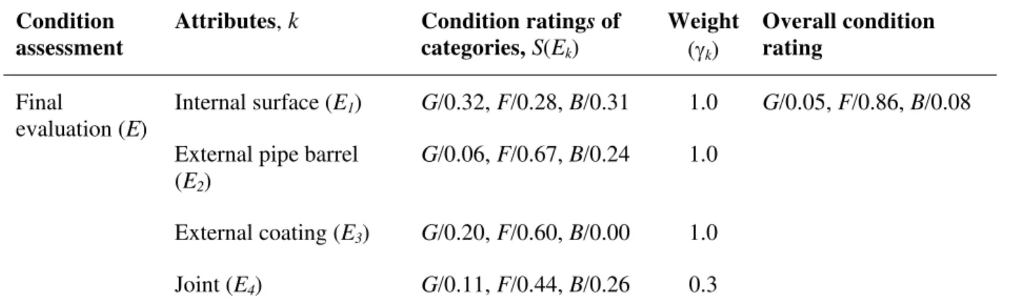
Evaluating an overall condition rating for the pipe system

The above section detailed how the condition rating for internal surface condition attribute is determined based on the information of distress indicators pertinent to that specific attribute. Similarly, contributions of the remaining three attributes such as external pipe barrel, external coating and joint conditions are determined. All four attributes are subsequently combined to obtain the overall condition rating.

As depicted in Figure 2, the four attributes can be written in terms of the factors identified

earlier, as ; ; ; and . Similarly,

the weight vectors for each factor are defined as ={ , , }; ={ , , , };

={ }; and = { , }. } { ₁1 ₁2 ₁3 1 e e e E = E₂ ={e1₂ e₂2 e₂3 e₂4} E₃={e1₃} E₄ ={e1₄ e₄2} 1 λ 1 1 λ 2 1 λ 3 1 λ λ₂ 1 2 λ 2 2 λ 3 2 λ 4 2 λ 3 λ 1 3 λ λ₄ 1 4 λ 2 4

λ Table 4 summarizes the attributes and contributory the factors that define the overall pipe condition rating of a lined cast iron pipe. Each attribute is evaluated using the same aggregation procedure described in section “illustrative evaluation of a category (an attribute): internal surface condition”. The overall condition assessment written in matrix form is ⎥ ⎥ ⎥ ⎥ ⎦ ⎤ ⎢ ⎢ ⎢ ⎢ ⎣ ⎡ = ⎥ ⎥ ⎥ ⎥ ⎦ ⎤ ⎢ ⎢ ⎢ ⎢ ⎣ ⎡ 19 . 0 26 . 0 44 . 0 11 . 0 20 . 0 00 . 0 60 . 0 20 . 0 03 . 0 24 . 0 67 . 0 06 . 0 09 . 0 31 . 0 28 . 0 32 . 0 4 3 2 1 E E E E (20)

The matrix on the right-hand side of the above equation represents the BPAs for each attribute (Ek). The columns of the matrix represent BPAs that correspond to condition states good, fair,

bad and ignorance (Table 5). The contribution of each of these attributes to the overall condition rating can be described by the use of importance weights, which are assigned based on experts'

judgment. We select the importance weight matrix as γk = {1, 1, 1, 0.3} for the lined cast iron

pipe. Using recursive D-S rule of combination, the first two attributes (E1γ1 ⊕ E2γ2) are combined to obtain{G 0.08,F 0.64,B 0.27}. This result is then combined with the third attribute (E1γ1 ⊕ E2γ2 ⊕ E3γ3) to obtain {G 0.06,F 0.85, B 0.08}. Finally, the latter result is

combined with the fourth attribute to obtain the overall condition rating (E) of a lined cast iron pipe as shown below

E(overall condition rating) = (E1γ1 ⊕ E2γ2 ⊕ E3γ3 ⊕ E4γ4) = {G 0.05, F 0.86,B 0.08} (21) Therefore, the most likely condition rating of this lined cast iron pipe is fair. It is also noted that the combined overall condition rating is very distinct from the condition rating based on one individual attribute or category. The epistemic uncertainty (ignorance) is now very low, i.e., 0.01, whereas the ignorance was in the 0.03 to 0.20 range for the four attributes (Eqn. 20).

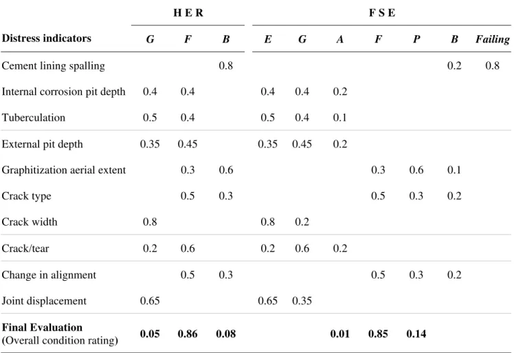
Rajani et al. (2006) proposed a fuzzy synthetic evaluation (FSE) model to determine the pipe condition rating. In their analysis, the authors employed seven condition states, namely,

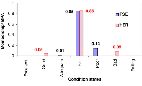
excellent, good, adequate, fair, poor, bad, failing for evaluation of pipe condition ratings instead of three as proposed in the HER model. The same data used to illustrate the HER model was repeated using the FSE model. Some simplified assumptions are made to map the data from three condition states to seven for the FSE model so that outcomes from both models can be compared. Table 6 summarizes the input data for each distress indicator used in the HER and FSE models and compares (Fig. 3) the overall condition ratings. The estimated overall condition ratings using FSE and HER models are {E/0, G/0, A/0.01, F/0.85, P/0.14, B/0, Failing/0} and {G/0.05, F/0.86, B/0.08}, respectively. The results obtained from FSE model are similar to the overall condition rating obtained by HER model in this case.

The proposed HER model can efficiently deal with situations that involve partial ignorance, inconsistencies and conflicts without making simplified assumptions. In case of FSE model, we have to make assumption to deal with incomplete evidence. The unassigned mass (membership) is assigned to contiguous condition state as can be seen in Table 6. For example, the condition rating of a buried pipe based on the measurements of crack width is in good condition with 80% degree of confidence. This is incomplete information; therefore remaining 20% will be assigned to ignorance without making any assumption. In case of FSE model, the remaining unassigned mass is shifted to the contiguous state so that the sum of the degree of membership function equal to 1.

The HER model is also comparatively more sensitive to perturbations and anomalies. For example, if some of the factors in the aggregation process are in bad condition and remaining factors are in good condition, the FSE model will evaluate that the overall condition rating as adequate/fair due to inherent assumption of weighted averaging in FSE model. However, the application of the HER model will manifest conflict, and shift the conflicting mass to ignorance BPA in the final evaluation. This will help the decision maker to understand the underlying mechanism of conflicting bodies of evidence, and provide more realistic evaluation of the pipe condition rating.

Conclusions

The condition rating of large-diameter water mains reflects an aggregate (overall) state of its health. Distress indicators are physical manifestations of the ageing process. The type (or form) and location of observed distress indicators in large-diameter mains are dependent on the pipe material, its surrounding environment and the cumulative effects of stresses to which it was

subjected. The physicochemical processes that promote ageing are yet not well understood (Rajani et al. 2006).

A pipe condition assessment method requires a rational, repeatable, and transparent approach. Evaluation process for pipe condition rating is a challenging task as it involves aggregation of diverse nature of contributing distress indicators to interpret an overall state of its health. The problem becomes increasingly complex due to uncertainties attributable to inherent subjectivity in the interpretation process. In this paper, a hierarchical evidential reasoning (HER) model is proposed for pipe condition assessment which can combine subjective, imprecise and

incomplete information, and even conflicting data. The HER model is based on Dempster-Shafer (D-S) rule of combination, which can combine multiple bodies of evidence by

incorporating both aleatory (variability, heterogeneity) and epistemic (incertitude, ignorance) uncertainties.

The proposed model (HER) is built systematically on condition assessment example for large diameter water mains. The results are compared with an existing algorithm based on fuzzy synthetic evaluation (FSE), proposed earlier by Rajani et al. (2006). One of the major advantages of using HER is that it has capability to deal with incomplete and conflicting evidence without making strong assumption about missing data as required in FSE. The HER model can combine multiple bodies of evidence provided they are obtained (or assumed) from independent sources. Because of its robust framework and its firm mathematical foundation, the HER model can be modified at any level of hierarchical structure without changing the recursive combination algorithm.

The basic algorithm used in the proposed model is based on D-S rule of combination, which assumes stochastic independence of sources avoids “conflicts” through normalization process (Marashi and Davis 2006). Many alternatives to this combination rule have been proposed in response to these two issues. To address “conflict” and “normalization”, various techniques including Yager (1987), Smets (1990), Inagaki (1991), Dubois and Prade (1992), Zhang (1994), Murphy (2000), and more recently by Dezert and Smarandache (2004) have been proposed. Marashi and Davis (2006) have also proposed an extension of D-S rule to deal with the problem of “dependence” using t-norm based combination rule.

In the real-world situation, the multiple factors (or attributes) that contribute to overall evaluation are generally dependent (or correlated), and may also provide highly conflicting evidence, which reduces the reliability of results in case of direct use of D-S rule of combination (Zadeh 1984). The present model is built on a hierarchical framework for pipe condition

assessment in which all contributory factors (or attributes) are assumed independent, and only the parallel aggregation of factors (or attributes) are performed using D-S rule of combination. The proposed model presented in this paper is still in infancy, and extensive work needs to be done to make algorithm HER more robust to deal with dependent factors as well as to

effectively deal with the issue of “conflict” using alternative rules of combination.

Acknowledgements

This work was part of a strategic research of National Research Council of Canada at the Institute for Research in Construction (NRC-IRC) in Ottawa. It was also partially supported by the National Natural Science Foundation of China (NSFC) under Grant No.60772077.

References

Attoh-Okine, N.O., and Gibbons, J. (2001). “Use of belief function in brownfield infrastructure redevelopment decision making.” ASCE Journal of Urban Planning and Development, 127(3), 126-143.

Chang, Y.C., and Wright, J.R. (1996). “Evidential reasoning for assessing environmental impact.” Civil Engineering Systems, 14(1), 55-77.

Chae, M-J., and Abraham, D.M. (2001). “Neuro-fuzzy approach for sanitary sewer pipeline condition assessment.” ASCE Journal of Computing in Civil Engineering, 15(1), 4-14. Dempster, A. (1967). “Upper and lower probabilities induced by a multi-valued mapping.” The

Annals of Statistics, 28, 325-339.

Dezert, J., and Smarandache, F. (2004). “Presentation of DSmT.” Advances and Applications of DSmT for Information Fusion (collected works), American Research Press, Rehoboth, 3-35.

Dingus, M., Haven, J., and Austin, R. (2002). “Nondestructive, non-invasive assessment of underground pipelines.” American Water Works Research Foundation, Denver, CO. Dubois, D., and Prade, H. (1992). “On the combination of evidence in various mathematical

frameworks.” Reliability Data Collection and Analysis, Ed. J. Flamm and T. Luisi, Brussels, ECSE, EEC, EAFC 213-241.

Duran, O., Althoefer, K., and Seneviratne, L.D. (2002). “State of the art in sensor technologies for sewer inspection.” IEEE Sensors Journal, 2(2), 73-81.

Fan, Xianfeng, Zuo, Ming J. (2006). “Fault diagnosis of machines based on D–S evidence theory Part 1: D–S evidence theory and its improvement.” Pattern Recognition Letters, 27, 366–

376.

Hutchinson, Tara C., Chen, Zhiqiang. (2006). “Improved image analysis for evaluating concrete damage.” ASCE Journal of Computing in Civil Engineering, 20(3), 210-216.

Inagaki, T. (1991). “Interdependence between safety-control policy and multiple sensor scheme via Dempster-Shafer theory.” IEEE Transactions on Reliability, 40(2), 182-188.

Kleiner, Y., Rajani, B., and Sadiq, R. (2005). “Risk management of large-diameter water transmission mains.” American Water Works Association Research Foundation, Denver, CO, 1-120.

Kuzniar Krystyna, and Waszczyszyn Zenon (2006). “Neural networks and principal component analysis for identification of building natural periods.” ASCE Journal of Computing in Civil Engineering, 20(6), 431-436.

Makar, J., and Chagnon, M. N. (1999). “Inspecting systems for leaks, pits, and corrosion.” Journal of American Water Works, 91(7), 36-46.

Marashi, E., and Davis, J.P. (2006). “An argumentation-based method for managing complex issues in design of infrastructural systems.” Reliability Engineering and System Safety, 91, 1535-1545.

Morcous, G., Rivard, H., and Hanna, A.M. (2002). “Case-based reasoning system for modeling infrastructure deterioration.” ASCE Journal of Computing in Civil Engineering, 16(2), 104-114.

Murphy, C.K. (2000). “Combining belief functions when evidence conflicts.” Decision Support Systems, 29, 1-9.

Naidu, A.S.K., Soh, C.K., and Pagalthivarthi, K.V. (2006). “Bayesian network for e/m

impedance-based damage identification.” ASCE Journal of Computing in Civil Engineering, 20(4), 227-236

Najjaran, H., Sadiq, R., and Rajani, B. (2006). “Fuzzy expert system to assess corrosivity of cast/ductile iron pipes from backfill properties.” Computer Aided Civil & Infrastructure Engineering, 21, 67-77.

Rajani, B., and Kleiner, Y., (2002). “Towards pro-active rehabilitation planning of water supply systems.” International Conference on Computer Rehabilitation of Water Networks CARE-W, Dresden, Germany, 29-38.

Rajani, B., Kleiner, Y., and Sadiq, R. (2006). “Translation of pipe inspection results into condition rating using fuzzy synthetic evaluation technique.” Journal of Water Supply: Research & Technology – AQUA, 55(1), 11-24.

Sadiq, R., Kleiner, Y., and Rajani, B. (2006). “Estimating risk of contaminant intrusion in distribution networks using Dempster-Shafer theory of evidence.” Civil Engineering and Environmental Systems, 23(3), 129-141.

Sentz, K., and Ferson, S. (2002). “Combination of evidence in Dempster-Shafer theory.” SAND 2002-0835.

Shafer, G. (1976). “A mathematical theory of evidence.” Princeton University Press, Princeton, N.J.

Sinha, S.K. (2004). “A multi-sensor approach to structure health monitoring of buried sewer pipelines infrastructure system.” Proceedings of the ASCE Pipeline Division Specialty Congress Pipeline Engineering and Construction, 1-11.

Smets, P. (1990). “The combination of evidence in the transferable belief model.” IEEE Transactions on Pattern Analysis and Machine Intelligence, 12(5), 447-458.

Wang, Y., and Civco, D.L. (1994). “Evidential reasoning-based classification of multi-source spatial data for improved land cover mapping.” Canadian Journal of Remote Sensing, 20, 381-395.

WEF (1994). “Existing sewer evaluation and rehabilitation.” Manual & Reports FD-6, ASCE Manuals & reports on engineering, No. 62.

Yager, R.R. (1987). “On the Dempster-Shafer framework and new combination rules.” Information Sciences, 41, 93-137.

Yang, J.-B., Xu, D.-L. (2002). “On the evidential reasoning algorithm of multiple attribute

decision analysis under uncertainty. ” IEEE Transactions on Systems Man and

Cybernatics, 32(3), 289-304.

Zadeh, L.A. (1984). “Review of books: A mathematical theory of evidence.” The AI Magazine, 5(3), 81-83.

Zhang, L. (1994). “Representation, independence, and combination of evidence in the Dempster-Shafer theory.” Advances in Dempster-Dempster-Shafer theory of evidence, Ed. Yager R.R.

Symbol list:

Ek kth attribute in the final evaluation i

k

e ith factor in the aggregation contributing to the kth attribute )

(i e

k

I combined set of i factors of the k th

attribute

Hn nth grade to which the state of an attribute may be evaluated

Lk number of the factors contributing to the kth attribute

M number of bodies of evidence

m(ei_k) basic probability assignment set for factor e_ki

m(e (i)) basic probability assignment for the combined set of i factors of the k

k I th attribute n H i k

m _, basic probability assignment assessed to grade Hn of ith factor in the kth attribute

n k

H j I

m _{( )} basic probability assignment for the jth combined set that is assessed to grade Hn

m(Ψ) basic probability assignment of the subset Ψ

m12(Ψ) combination basic probability assignment of two sets, m1(Ψ) and m2(Ψ)

N the number of evaluation grade (condition states)

S(ei_k) evaluation for a factor ei_k

βn,i degree of confidence assigned to the grade Hn of the ith factor

Φ empty (void) set

i k

λ normalized relative weight of factoreki contribute to attribute Ek Θ, H frame of discernment (universe of discourse)

Figure captions:

Fig. 1. Generic framework for the proposed HER model

Fig. 2. Hierarchical framework for condition assessment of cast/ductile iron pipes

⊕ ⊕ ⊕ Attribute level Factor level …

Model inputs for assigning BPA to different factors 1 k e m( 1 k e )= S(e )×1k 1 k λ m( Lk k e )=S( Lk k e )× lk k λ Final evaluation E1 1 1 e 1 1 L e m( 1 1 e )= S( 1 1 e )×λ m(11 11 L e )= S( 1 1 L e )× 1 1 L λ Ek k L k e … …

Final evaluation Attribute level Factor level

Cement lining spalling

Internal surface

condition (E1) Internal corrosion pit depth

Tuberculation

External pit depth

Graphitization aerial extent Overall pipe condition rating (E) External pipe barrel condition (E2) Crack type Crack width External coating condition (E3) Crack/tear Change in alignment Joint condition (E4) Joint displacement

Figure 2. Hierarchical framework for condition assessment of cast/ ductile iron pipes

0.01 0.14 0.08 0.86 0.05 0.85 0 0.2 0.4 0.6 0.8 1 Excellent Good Adequate

Fair _Poor Bad

Failing Condition states Mem bership/ BPA FSE HER

Table 1. Evaluation of the contributory factors for the attribute of joint condition

The values in the matrix represent degree of confidence.

Contributory factors good (H1) fair (H2) bad (H3) ignorance (H) Joint displacement 0.9 ⎯ ⎯ 0.1

Table 2. The D-S rule of combination for two bodies of evidence

Second body of evidence (factor), m

( )

Joint body of evidence ( )

(

)

( )

First body of evidence (factor),

1 1 e m {H} {H1}/ (m_kH_,1 1) 2 , H k m … {Hn}/ (m_kH_,1 Hn) k m _,2 … {HN}/ (m_kH_,1 HN ) k m _,2 {H}/ (m_kH_,1 m_kH_,2)

Table 3. Evaluation of internal surface condition of a lined cast iron pipe Attribute, k = 1 Contributory factors, i = 1, 2, 3 Distress indicator status Condition rating, S(e₁i)

Cement lining spalling (e₁1) Yes B/0.8

Internal corrosion pit depth (e₁2) 30% < Pit depth < 60% G/0.4, F/0.4

Internal surface condition (E1)

Tuberculation (e₁3) Diameter reduced

by < 20%

G/0.5, F/0.4

The evaluation grades for the related factors are defined as {good(G)/β, fair(F)/β, bad(B)/β}, where β represents the degree of confidence.

Table 4. Summary of attributes and contributory the factors that define the overall condition rating of a lined cast iron pipe

Attributes, k Contributory factors, i Condition ratings of distress indicators, S(ei_k)

Weight,

(λi_k)

Cement lining spalling (e₁1) B/0.80 1.0

Internal corrosion pit depth (e₁2) G/0.40, F/0.40 1.0

Internal surface

(E1)

Tuberculation (e₁3) G/0.50, F/0.40 0.6

External pit depth (e1₂) G/0.35, F/0.45 1.0

Graphitization aerial extent (e₂2) F/0.30, B/0.60 1.0

Crack type (e3₂) F/0.50, B/0.30 1.0 External pipe barrel (E2) Crack width (e₂4) G/0.80 0.6 External coating (E3) Crack/tear (e1₃) G/0.20, F/0.60 1.0 Change in alignment (e1₄) F/0.50, B/0.30 1.0 Joint (E4) Joint displacement (e₄2) G/0.65 0.6

The evaluation grades for the related factors are defined as {good(G)/β, fair(F)/β, bad(B)/β}, where β represents the degree of confidence.

Table 5. Final evaluation of pipe condition rating

Condition assessment

Attributes, k Condition ratings of

categories, S(Ek) Weight (γk) Overall condition rating Internal surface (E1) G/0.32, F/0.28, B/0.31 1.0

External pipe barrel

(E2) G/0.06, F/0.67, B/0.24 1.0 External coating (E3) G/0.20, F/0.60, B/0.00 1.0 Final evaluation (E) Joint (E4) G/0.11, F/0.44, B/0.26 0.3 G/0.05, F/0.86, B/0.08

The evaluation grades for the related factor are defined as {good(G)/β, fair(F)/β, bad(B)/β}, where β represents the degree of confidence.

Table 6. Summary of input information used to compare FSE and HER models to evaluate overall condition ratings of the lined cast iron pipe

H E R F S E

Distress indicators G F B E G A F P B Failing

Cement lining spalling 0.8 0.2 0.8

Internal corrosion pit depth 0.4 0.4 0.4 0.4 0.2

Tuberculation 0.5 0.4 0.5 0.4 0.1

External pit depth 0.35 0.45 0.35 0.45 0.2

Graphitization aerial extent 0.3 0.6 0.3 0.6 0.1

Crack type 0.5 0.3 0.5 0.3 0.2 Crack width 0.8 0.8 0.2 Crack/tear 0.2 0.6 0.2 0.6 0.2 Change in alignment 0.5 0.3 0.5 0.3 0.2 Joint displacement 0.65 0.65 0.35 Final Evaluation

(Overall condition rating) 0.05 0.86 0.08 0.01 0.85 0.14

In hierarchical evidential reasoning (HER) model, the frame of discernment for condition states of a pipe is defined as {good(G), fair(F), bad(B)}; in fuzzy synthetic evaluation (FSE) model, the frame of discernment (universe of discourse) for condition states of a pipe is defined as {excellent(E), good(G), adequate(A), fair(F), poor(P), bad(B),