Automatic identification of artifacts in electrodermal activity data
The MIT Faculty has made this article openly available.
Please share
how this access benefits you. Your story matters.
Citation
Taylor, Sara, Natasha Jaques, Weixuan Chen, Szymon Fedor, Akane
Sano, and Rosalind Picard. “Automatic Identification of Artifacts
in Electrodermal Activity Data.” 2015 37th Annual International
Conference of the IEEE Engineering in Medicine and Biology Society
(EMBC) (August 2015), 25-29 Aug. 2015, Milan, Italy. pp.1934-1937.
As Published
http://dx.doi.org/10.1109/EMBC.2015.7318762
Publisher
Institute of Electrical and Electronics Engineers (IEEE)
Version
Author's final manuscript
Citable link
http://hdl.handle.net/1721.1/103781
Terms of Use
Creative Commons Attribution-Noncommercial-Share Alike
Automatic Identification of Artifacts in Electrodermal Activity Data
Sara Taylor
1∗, Natasha Jaques
1∗, Weixuan Chen
1, Szymon Fedor
1, Akane Sano
1and Rosalind Picard
1Abstract— Recently, wearable devices have allowed for long term, ambulatory measurement of electrodermal activity (EDA). Despite the fact that ambulatory recording can be noisy, and recording artifacts can easily be mistaken for a physiological response during analysis, to date there is no auto-matic method for detecting artifacts. This paper describes the development of a machine learning algorithm for automatically detecting EDA artifacts, and provides an empirical evaluation of classification performance. We have encoded our results into a freely available web-based tool for artifact and peak detection.
I. INTRODUCTION
Electrodermal Activity (EDA) refers to the electrical po-tential on the surface of the skin [1]. When the body responds to stress, temperature, or exertion, the sympathetic nervous system (SNS) increases sudomotor innervation, causing EDA to increase and perspiration to occur. Because the SNS is influenced by the hypothalamus and limbic system — structures in the brain that deal with emotion — EDA has frequently been used in studies related to affective phenomena and stress (e.g. [5], [6], [7], [8], [10], [12], [14]). Despite its popularity, little research has been done into detecting noise and artifacts in an EDA signal. This is especially problematic given the increasing number of studies that are collecting ambulatory EDA data over long time periods using wearable devices (e.g. [2] [5] [7] [11] [14]). While these studies may provide profound insight into how affect and stress interact with other factors in daily life, continuous and unobtrusive measurement of EDA using wearable devices makes the signal collected vulnerable to several types of noise. Artifacts can be generated from electronic noise or variation in the contact between the skin and the recording electrode caused by pressure, excessive movement, or adjustment of the device. If these artifacts remain in the signal when it is analyzed they can easily be misinterpreted and skew the analysis; for example, they may be mistaken for a skin conductance response (SCR) (a physiological reaction that may indicate increased stress).
Consequently, many researchers are forced to manually inspect the data in order to decide which portions are too noisy to retain (e.g. [3]). This approach cannot scale to the type of large-scale EDA studies that are currently being proposed [7], which may involve data collected from hun-dreds of participants over weeks or months. In order to make collecting EDA viable in these types of studies, an automated
*Both authors contributed equally to this work
1Affective Computing Group, Media Lab, Massachusetts
Institute of Technology, 75 Amherst Street, Cambridge, U.S. {sataylor, jaquesn, cvx, sfedor, akanes, picard}@media.mit.edu
method for detecting and removing noise and artifacts must be developed. In this paper we describe the development of both a classification algorithm for automatically detecting artifacts, and an online system hosted at eda-explorer. media.mit.edu that will apply the algorithm to users’ uploaded EDA files in order to provide them with an analysis of which portions contain artifacts.
II. RELATED WORK
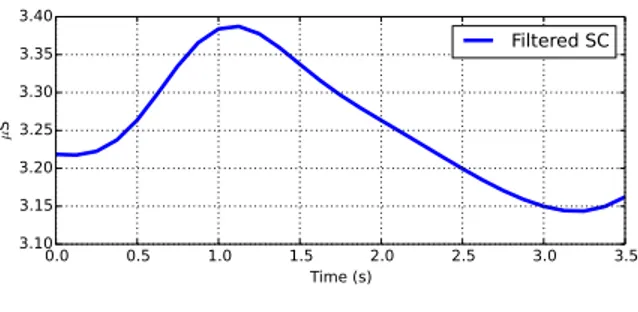
Through extensive research into the physiological pro-cesses underlying EDA, as well as the electrical properties of the recording equipment used in measurement, Boucsein [1] is able to provide a complete description of the characteristic shape of an SCR: the response typically lasts between 1-5 seconds, has a steep onset and an exponential decay, and reaches an amplitude of at least .01µS (see Fig. 1 for an example of a typical SCR). However, despite the availability of this knowledge, no accepted technique for removing signal artifacts has been developed.
0.0 0.5 1.0 1.5 2.0 2.5 3.0 3.5 Time (s) 3.10 3.15 3.20 3.25 3.30 3.35 3.40 µ S Filtered SC
Fig. 1. Shape of a typical SCR
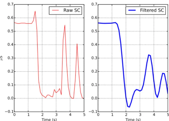
Currently, many researchers deal with signal artifacts and noise by simply applying exponential smoothing (e.g. [6]) or a low-pass filter (e.g. [8] [9] [12]). While these techniques are able to smooth small variations in the signal, they are not able to compensate for large-magnitude artifacts that can result from pressure or movement of the device during ambulatory recording. Fig. 2 shows a portion of signal that contains three obvious artifacts, in which the sharp decreases could not possibly be produced by human physiology. As is evident from comparing the raw and filtered versions of the signal, the low-pass filter has not removed the artifacts, and any subsequent analysis based on the filtered signal is likely to mistake the artifacts as genuine physiological responses.
Other researchers have used Boucsein’s analysis to de-velop heuristic techniques for removing atypical portions of the EDA signal. Kocielnik and colleagues [8] chose to discard portions of their data where the signal increased more than 20% per second or decreased more than 10% per
0 1 2 3 4 5 Time (s) −0.1 0.0 0.1 0.2 0.3 0.4 0.5 0.6 0.7 µ S Raw SC 0 1 2 3 4 5 Time (s) −0.1 0.0 0.1 0.2 0.3 0.4 0.5 0.6 0.7 Filtered SC
Fig. 2. A portion of the signal containing artifacts. The raw signal is shown on the left; a 1Hz low-pass filter has been applied to the signal on the right.
second. They verified that this approach removed artifacts based on visual inspection. Using a similar approach, Storm and colleagues manually set thresholds for the maximum and minimum amplitude, maximum slope, and minimum width of an SCR, and discarded responses that did not fit these criteria [13]. In another case, a study which collected EDA from two sensors (on both the ankle and the wrist) was able to detect artifacts by looking for epochs when only one of the two sensors had an abnormally low signal, or showed an unusually rapid increase or decrease [5].
These heuristic thresholds were developed for particular studies and participants, and verified only through visual inspection by the researchers conducting them; they may not generalize beyond those contexts. We seek to develop an empirically validated automatic technique for removing artifacts in EDA signals.
III. METHODS
In order to validate our automatic artifact detection method, we needed to establish a ground truth for what portions of an EDA signal are considered clean, and what portions contain artifacts. To do this we had two expert EDA researchers label 5-second epochs of EDA data collected from a previous experiment [3]. The labeled data was used as input to our machine learning classifier.
A. Data Collection
The data used in this analysis were collected during a study in which 32 participants completed physical, cognitive and emotional tasks while wearing Affectiva Q EDA sensors on both wrists [3]. The Q sensor collects EDA data by measuring skin conductance (SC) in microSiemens (µS) at a frequency of 8Hz. All experimental procedures were ap-proved by the Institutional Review Board for human subjects research at MIT.
B. Expert Labeling
We created a data set of 1560 non-overlapping 5-second epochs of EDA data, sampled from portions of data that were identified as possibly containing artifacts, true SCRs, or static skin conductance level (SCL). As part of our website, we built an interface to allow our two experts to review these epochs and assign a label of either ‘artifact’ or ‘clean’. Both experts agreed on a set of criteria that defines an artifact in the signal, which is as follows:
• A peak which does not show exponential decay, de-pending on the context (e.g. if two SCRs occur close together in time, the first response may not decay before the second begins, yet this is not considered an artifact) • Quantization error with ≥ 5% of signal amplitude • A sudden change in EDA correlated with motion • A SCL ≤ 0
Although our classification labels were created using these criteria, our website provides the ability for other researchers to agree to label their own data according to their individual application needs. The site allowed the experts to view both the raw signal and a filtered signal (to which a standard 1Hz low-pass filter had been applied), as well as the accelerometer data, which is simultaneously collected by the Q sensor. We felt that viewing the accelerometer data might help the experts to identify motion artifacts. However, we do not provide acceleration data to our classification algorithm, for two reasons. Firstly, by training the classifier using only EDA data, we enable it to be applied to EDA signal collected from devices other than the Q that do not collect accelerometer data. Secondly, while it would be simple to discard por-tions of the signal with high power in the corresponding accelerometer data, this is not always desirable; for example, in applications such as detecting epileptic seizures, strong accelerometer signal occurs simultaneously with high EDA, but the EDA signal is both clean and valuable to the analysis [9]. Because we allowed the raters to skip epochs if they did not wish to label them, we eventually obtained 1301 data points that were labeled by both experts. The percentage agreement was 80.71%, and the Cohen’s κ = 0.55.
There are multiple ways to deal with epochs for which the raters’ labels did not agree. The first is to discard them, which is reasonable in the sense that we cannot establish a ground truth value for those epochs, meaning we have no way to train or assess the performance of the classifier. The second technique is to treat disagreements as a third class in which we are unsure whether the signal is clean or an artifact. We will present results from both approaches. Table I gives the datasets for both.
TABLE I
NUMBER OFEPOCHS IN EACH CLASSIFIER
Classifier # Clean Epochs # Questionable Epochs # Artifact Epochs Binary 798 NA 252 Multiclass 798 251 252
C. Feature Extraction
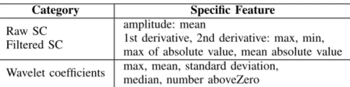
We extracted several features for each five second epoch. Given the importance of the shape of an SCR, we began by including statistics related to the amplitude and first and second derivative of the EDA signal (see Table II). These features were computed for both the raw and filtered signal; we are not concerned about including too many features at this stage, because we later apply a feature selection procedure to reduce the chance of overfitting.
TABLE II
COMPUTEDFEATURES
Category Specific Feature Raw SC
Filtered SC
amplitude: mean
1st derivative, 2nd derivative: max, min, max of absolute value, mean absolute value Wavelet coefficients max, mean, standard deviation,
median, number aboveZero
We then used a Discrete Haar Wavelet Transform to compute additional features that may be indicative of sudden changes in the EDA signal. Wavelet Transforms have been successfully used in several noise reduction applications; be-cause of their good time-frequency localization, they can be considered a spatially aware noise filtration technique [15]. A wavelet transform decomposes a signal into coefficients at multiple scales; in our case, we obtain coefficients at 4Hz, 2Hz, and 1Hz. Because the Haar wavelet transform involves computing the degree of relatedness between subsequent points in the original signal, it is excellent for detecting edges and sharp changes [15]. Using this technique applied to the participant’s full EDA signal, the 3 levels of detail coefficients were computed, and statistics were computed on the coefficients over each 5-second epoch.
D. Feature Selection
Because we computed a large number of potentially redun-dant features, we used wrapper feature selection to ensure that our classifier did not overfit the training data. Unlike simple filtering techniques that merely rank features based on their relationship to the classification label, Wrapper feature selection (WFS) repeatedly tests subsets of features using a specific classifier1in order to select an independent subset of features that work well in combination with each other [4]. Since this is computationally expensive, we used a greedy search process, which can quickly search the space of all subsets and is robust to overfitting [4].
E. Classification
In order to perform feature and model selection, we partitioned the data set into training, validation, and testing sets, using a randomized 60/20/20% split. Feature selection was performed using only the training data. In order to find a suitable machine learning technique for this problem, we tested a variety of algorithms including neural networks, 1WFS was used with SVM after it was found to be the most effective
algorithm
random forests, na¨ıve Bayes, nearest neighbour, logistic re-gression, and support vector machines (SVM). The algorithm that produced the best accuracy on the validation data set was SVM, so we focus on SVM for the remainder of the paper. In order to perform model selection we tested a range of settings for the parameters of SVM, including both a Radial Basis Function (RBF), polynomial, and linear kernel, and selected the settings that produced the highest accuracy on the validation set. The held-out test set was not used in feature or model selection.
IV. RESULTS A. Classification results
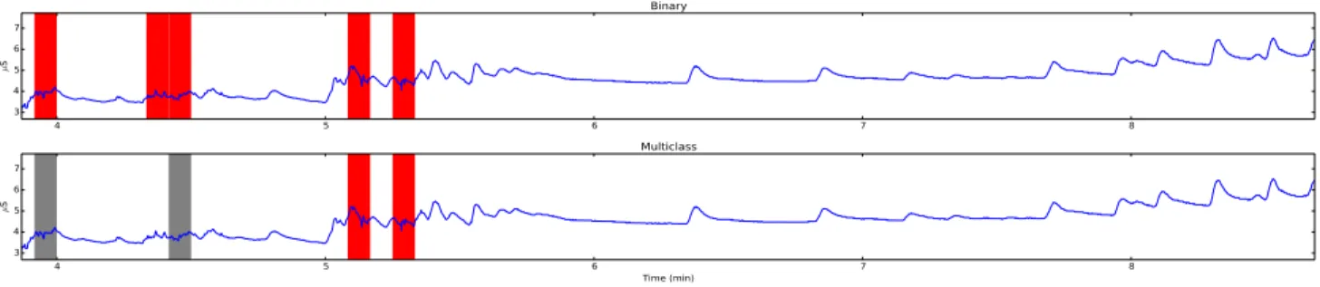
Table III shows the classification results obtained for both the binary and multiclass classifiers on the validation and test sets, as well as the optimal SVM parameters. Although the accuracy for the multiclass classifier is lower (three-class (three-classification is a more difficult problem), the output may prove more useful for real users. Fig. 3 shows both algorithms applied the same portion of EDA signal. As is evident from the figure, portions of the signal containing artifacts are detected (in red), while normal SCRs are labeled clean. Fig. 4 shows the performance of the algorithms on another sample containing a greater number of artifacts, which are also detected by both algorithms. The multiclass algorithm is able to label questionable parts of the data that are not clear artifacts in grey. Note that the binary classifier labels some epochs as artifacts that the multiclass one does not. The level of stringency needed in the classifier may depend on the researchers’ application; computing aggregate measures like area under the curve may be less sensitive to artifacts than SCR detection.
TABLE III
CLASSIFIER SETTINGS AND ACCURACY RESULTS
Classifier Parameter settings Baseline Accuracy Validation Accuracy Test Accuracy Binary RBF, β=0.1, C=1000 76.0% 96.95% 95.67% Multiclass RBF, β=0.1, C=100 61.33% 88.38% 78.93% B. Features selected
The feature selection process only led to a marginal improvement in classification on the validation set: 1.3% and 1.4% for the binary and multiclass classifiers, respectively. However the features selected provide valuable insight into the signal characteristics that best distinguish between nor-mal EDA and an artifact. Table IV shows the features se-lected by the binary classifier; the multiclass version sese-lected extremely similar features. The selected features confirm the theoretical assumption that shape, including first and second derivative, are important in detecting artifacts. The wavelet features also proved valuable, especially the standard deviation of the coefficients. This is intuitive, because these values indicate whether there is a change in the wavelet domain, which may be indicative of an edge or sharp change in the original signal.
4 5 6 7 8 3 4 5 6 7 µ S Binary 4 5 6 7 8 Time (min) 3 4 5 6 7 µ S Multiclass
Fig. 3. A subset of a single participant’s data which includes true SCRs and artifacts. The red and grey shading shows epochs labeled as artifact and unsure, respectively. We note that both classifiers label true SCRs as clean signal.
75.4 75.6 75.8 76.0 76.2 0.0 0.5 1.0 1.5 2.0 2.5 3.0 µ S Binary 75.4 75.6 75.8 76.0 76.2 Time (min) 0.0 0.5 1.0 1.5 2.0 2.5 3.0 µ S Multiclass
Fig. 4. An example of a typical artifact similar to Fig. 2 when the participant removed the sensor. Red and grey shading show where the classifiers labeled the SC data as artifact and questionable, as respectively.
TABLE IV
FEATURESSELECTED FORBINARYCLASSIFICATION
Category Specific Feature Raw SC
amplitude: mean
1st derivative: max absolute value 2nd derivative: max, mean absolute value Filtered SC amplitude: mean
2nd derivative: min, max absolute value Wavelet
Mean: 1st coefficient
St. Dev: 1st, 2nd, 3rd coefficients Median: 3rd coefficient
V. CONCLUSION
In summary, we have developed algorithms that can au-tomatically and accurately distinguish artifacts in an EDA signal from normal physiological responses. The code we have written to develop these algorithms is freely available on our website, and we are currently extending the site so that anyone will be able to upload their raw EDA signal and re-ceive an output indicating which portions contain noise. This tool could be enormously time-saving to researchers dealing with large data sets involving many participants measured over long periods of time. In the future we hope to extend
our approach using active, semi-supervised learning, which will allow the machine learning algorithm to interactively ask the user to label specific epochs based on its level of uncertainty. This way, human raters will be required to label fewer epochs that are highly similar, and instead will only label novel data for which the classifier has little information.
ACKNOWLEDGMENT
This work was supported by the MIT Media Lab Con-sortium, Samsung, NIH Grant R01GM105018, Canada’s NSERC program, and the People Programme (Marie Curie Actions) of the European Union’s Seventh Framework Programme FP7/2007-2013/ under REA grant agreement #327702.
REFERENCES
[1] W. Boucsein. Electrodermal activity. Springer Science+Business Media, LLC, 2012.
[2] S. Doberenz et al. Methodological considerations in ambulatory skin conductance monitoring. Int. J. of Psychophysiology, 80(2):87–95, 2011.
[3] S. Fedor and R. Picard. Ambulatory eda: Comparisons of bilateral forearm and calf locations. 51:S76–S76, 2014.
[4] I. Guyon and A. Elisseeff. An introduction to variable and feature selection. J. of Machine Learning Research, 3:1157–1182, 2003. [5] E. B. Hedman. In-situ measurement of Electrodermal Activity during
Occupational Therapy. PhD thesis, MIT, 2010.
[6] J. Hernandez, R. R. Morris, and R. W. Picard. Call center stress recognition with person-specific models. In ACII, pages 125–134. Springer, 2011.
[7] C. Kappeler-Setz et al. Towards long term monitoring of electrodermal activity in daily life. Pers. ubiquit. comput., 17(2):261–271, 2013. [8] R. Kocielnik et al. Smart technologies for long-term stress monitoring
at work. In Comput.-Based Medical Syst., pages 53–58. IEEE, 2013. [9] M.-Z. Poh. Continuous assessment of epileptic seizures with
wrist-worn biosensors. PhD thesis, MIT, 2011.
[10] T. Reinhardt et al. Salivary cortisol, heart rate, electrodermal activity and subjective stress responses to the mannheim multicomponent stress test (mmst). Psychiatry research, 198(1):106–111, 2012.
[11] A. Sano et al. Discriminating high vs low academic performance, self-reported sleep quality, stress level, and mental health using personality traits, wearable sensors and mobile phones. In Body Sensor Networks (BSN) (to appear), 2015.
[12] A. Sano and R. Picard. Stress recognition using wearable sensors and mobile phones. In ACII, pages 671–676. IEEE, 2013.
[13] H. Storm et al. The development of a software program for analyzing spontaneous and externally elicited skin conductance changes in infants and adults. Clin. Neurophysiology, 111(10):1889–1898, 2000. [14] F. H. Wilhelm and W. T. Roth. Taking the laboratory to the skies: Ambulatory assessment of self-report, autonomic, and respiratory responses in flying phobia. Psychophysiology, 35(5):596–606, 1998. [15] Y. Xu et al. Wavelet transform domain filters: a spatially selective