Asymmetric Modes of Elastic Wave Propagation in a Fluid-Filled Borehole

FINITE DIFFERENCE SYNTHETIC ACOUSTIC LOGS

FOR BOREHOLES WITH SHARP, ROUGH INTERFACES

by R.A. Stephen

P.O.

Box 567

West Falmouth, MA 02547

ABSTRACT

Previous finite difference codes developed for this consortium were unstable at rough, sharp liquid-solid interfaces. In this paper we present results from a method developed by Nicoletis (1981) and Bhasavanija (1983) which is stable at rough, sharp liquid-solid interfaces. The method gives acceptable accuracy for the vertically homogeneous case when compared with discrete wavenumber results. Examples are also given for waShouts and horizontal fissures with sharp liquid-solid boundaries. Head waves tend to follow the shape of the borehole wall in the washout examples, but are greatly attenuated at fissures. In the fissure case, pseudo-Rayleigh waves are reflected from the fissure, but Stoneley waves are almost unaffected.

INTRODUCTION

This paper is the third in· a· series on finite difference synthetic acoustic logs. The first paper (Stephen et al., 1983) introduced a finite difference code for the acoustic logging problem and the second paper (Stephen and Pardo-Casas, 1984) demonstrated the applicability of the method to acoustic logging problems with vertically varying velocity and density profiles. The code used in these papers was stable and accurate at flat (vertical), sharp interfaces and at two-dimensionally varying interfaces where the transition in elastic parameters was smooth. In the first case boundary conditions were specifically coded (the boundary condition method) and in the second case solutions were obtained directly from the elastic wave equation for heterogeneous media (the Stephen method). It is too inconvenient to specifically code boundary conditions for non-planar, or even piecewise planar, interfaces. At sharp interfaces, where the elastic parameters varied from liquid to solid over a few grid points, the finite difference formulation of the wave equation for heterogeneous media was unstable.

In this report we show the results of a scheme developed by Nicoletis (1981) and Bhasavanija (1983) which is stable for rough, sharp interfaces and has acceptable accuracy.

Bhasavanija (1983) applied the method to the acoustic logging problem by considering examples consisting of homogeneous blocks. He applied his code for heterogeneous media to the edges and corners of the blocks, and used the traditional code for homogeneous media inside the blocks. (The Bhasavanija code reduces to the traditional code in homogeneous media). At the borehole wall he used

102

Stephen

the space increments.

Our application of the formulation differs from Bhasavanija (1983) in two respects. First, we use the general Bhasavanija formulation at every point in the "transition" region (Figure 1). In homogeneous sections in the transition region we get the traditional formulation by default. However, by applying the Bhasavanija formuiation everywhere we can handle general sharp interfaces and gradients without changing the code. The second difference is that we also use the general Bhasavanija formulation at the liquid-solid borehole wall, without applying a specific boundary condition code. We no longer define two components of tangentiai displacement at the interface to allow for slip. Although there is a logical inconsistency in doing this, comparison of results with other methods suggests that this is not serious. We suggest that the Bhasavanija method can be used for general fluid-solid transitions consisting of sharp or gradual contrasts in one or two dimensions.

THE METHOD OF NICOLETIS AND BHASAVANIJA

The new finite difference formulation, which we refer to as the Bhasavanija method, is outlined by Nicoletis (1981) and Bhasavanija (1983). Although there are some typographical errors, particularly in the latter reference, we refer the reader to these papers for details of the method. The essential feature which distinguishes the Bhasavanija formulation from the Stephen formulation (Stephen et al., 1983) is the manner in which elastic parameters and particle displacements are defined on the grid (Figure 2). In the Stephen method, which follows earlier formulations by Alterman and Karal (1968) and others, the elastic parameters and particle displacements are defined at the same grid points. In the Bhasavanija scheme the elastic parameters are defined at grid points which are offset by half a grid increment (in radius and depth) from the grid points for particle displacement. The averaging which is then necessary in the finite difference scheme leads to remarkably good accuracy for acoustic logging problems. Results are compared with the discrete wavenumber method and the original boundary condition finite difference method (Stephen et al., 1983) for vertically homogeneous media to confirm the accuracy. A comparison between the Stephen and Bhasavanija methods for steep gradients is presented to demonstrate where the accuracy of the former method breaks down. Examples of washouts and fissures with sharp boundaries are also discussed.

The previous papers discussed only hard formation examples

(v..

>

VI)'

so for completeness we are including in the Appendix some examples of propagation in soft formations

(V$

<

VI)'

Model Parameters

In order to facilitate comparison, model sizes and source frequencies are the same as in the previous papers. Figure 1 shows the geometry used for the calculations. Unless otherwise noted, all models considered are 0.6 m wide by 3.0 m long (60 grid points by 300 grid points at 0.01 m per grid point) and time series are generated out to 2.5 msec (1250 time steps at 0.002 msec per step). A compressional point source is located at the center of a 0.1 m radius borehole and receivers are placed at the center of the borehole at increments of 0.2 m between

Stephen and Pardo-Casas (1984). The center frequency in pressure is 15 kHz and the upper half-power frequency is 20 kHz.

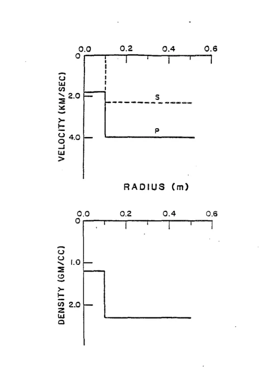
NUMERICAL EXAMPLES The Vertical Liquid- olid Interface

As an initial test of the Bhasavanija scheme we ran the same sharp interface example as discussed in the previous papers (Figure 3a). Figure 3b compares the discrete wavenumber and boundary condition finite difference codes. (Figure 3b was presented in an earlier paper.) Comparison of the Bhasavanija scheme (which does not allow slip at the Interface) with the boundary condition method (which does specifically allow slip) shows acceptable agreement for all phases (Figure 3c). We have no explanation for the apparent unimportance of the slip condition in this model. The snapshots and a discussion of the various arrivals for this model were given in Stephen and Pardo-Casas (1984).

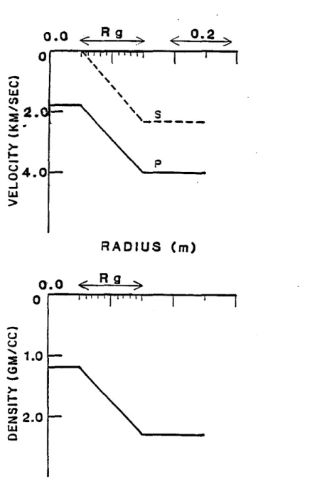
Vertically Homogeneous Gradients between the Borehole Fluid and the Formation In this series of examples we compare the Stephen and Bilasavanija schemes for a range of gradients between the liquid and the homogenecus solid. This emphasizes the stability of the Bhasavanija scheme, shows the magnitude of gradient at which the Stephen scheme breaks down, and demonstrates the range of effects one might see in field data from regions where gradient models are applicable. In Figure 4, results are presented for the two methods when the transition width between liquid and solid (Rg) varies from 0.03 to 0.20 m.

The nature of the instability of the Stephen scheme at liquid-solid interfaces can be seen at widths 0.03 and 0.05 m (Figure 4b). The onset time of the instability is a function of gradient. At a width of 0.01 m no useful results are obtained. It appears that the liquid-solid contrast is always unstable but that the rise time of the instability depends on the velocity contrast immediately at the borehole wall.

Good agreement in compressional head waves and leaky PI. modes is obtained by a width of 0.07 m and in guided waves by a width of 0.15 m. However, even at 0.20 m there are still discrepancies in the guided wave packet. These are probably caused by the slight increase in borehole radius (0.005m) for the Bhasavanija case, caused by the manner in which the eiastic parameters are defined (Figure 2).

The Washout with a Sharp Interface

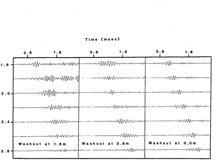
As in the previous paper (Stephen and Pardo-Casas, 1984) we consider washouts at three depths relative to the source (Figure 5). In these examples the pseudo-Rayleigh wave has significant amplitude (because of the shear coupling) and the PI. modes are very diminished (since "diving ray" or body wave energy plays no role in this case).

104

Stephen

examples for deeper washouts (0.8 and 1.6 m) indicating that once generated, they follow the shape of the borehole. Frequency-wavenumber analysis should be pursued to more fully understand the complicated behavior in the guided waves.

The Bhasavanija code Is a little noisy for the case with the washout at 1.6 m. This is best illustrated by comparing the microseismograms at 1.6 m for the washout at 0.0 m and at 1.6 m. By reciprocity, these two microseismograms should be identical, as demonstrated in Stephen and Pardo-Casas. In this paper, the early parts of the microseismograms are identical; however, there are significant differences between the two past about 1.2 msec. We attribute this to numerical noise. This numerical noise appears to arrive late in the microseismogram and does not seem to affect the body and guided wave packets.

The Horizontal Fissure with Sharp Edges

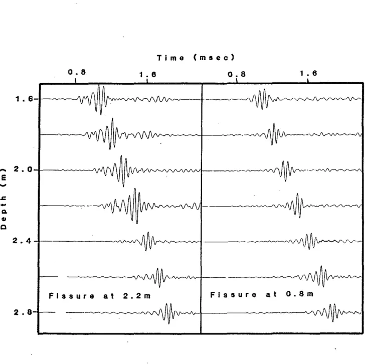
As in the washout case, by studying the sharp interface model we can see the effects of fissures on the shear and pseUdo-Rayleigh waves, as well as the compressional and Stoneley wave (Figure 6). The dramatic effect demonstrated here is that a 10 cm wide fissure almost totally reflects the pseudo-Rayleigh wave but is more transparent to the Stoneley wave. The reflected pseudo-Rayleigh wave can be clearly seen in the case of the fissure at 2.2 m. For the fissure at 0.8 m, almost all the guided wave energy below the fissure is in the Stoneley wave. Head wave energy is greatly attenuated at the fissure with sharp interfaces.

Computational Time

The Bhasavanija formulation does more calculations than the Stephen formulation. For the model described above with a transition zone width of 40 grid points, the Bhasavanija scheme required 162 minutes of CPU time compared to 118 minutes for the Stephen scheme (on a VAX 11-780 with VMS). The comparison is obviously very dependent on transition zone width.

CONCLUSIONS

The Bhasavanija formulation Is an acceptable finite difference scheme for wave propagation in boreholes with sharp, rough interfaces. The slight degradation in accuracy is compensated by the ease and convenience of the new method.

Application of the method shows that horizontal fissures essentially filter pseudo-Rayleigh from Stoneley waves. The pseudo-Rayleigh waves are almost totally· reflected at the fissure and the Stoneley waves are almost totally transmitted. Paillet (1984) observed reflections from a fracture for both Stoneley and pseudo-Rayleigh waves in field data. The reflections of either of both guided waves may be a function of the width and other fracture parameters. For smooth changes in borehole radius, head waves follow the shape of the well.

ACKNOVVLEDGEMENTS

This research is supported by the Full VVaveform Acoustic Logging Consortium at M.LT.

106

stephen

APPENDIX: SLOW FORMATIONS

For the model dimensions described above, slow formation examples have presented difficulties. We consider here a sharp interface (using the boundary condition formulation) between a fluid filled borehole and a soft formation with

v"

<

V

_J. Instabilities arise from the right hand absorbing boundary if Poisson's ratio is significantly higher than 0.25. These occur at large times after the initially incident energy was absorbed.

Figure A-1 is an example of the problem. The high frequency energy at the end of the traces is numerical noise arising from the absorbing boundary after the initial body waves have been absorbed. The two solutions around the problem are to use a larger grid or to keep Poisson's ratio at the boundary closer to 0.25.

Figure A-2 shows the solution to the problem using a larger grid. The right hand boundary is far enough away that any instabilities there do not have time to effect the solution. The solution consists almost entirely of the compressional head wave and PL modes with a phase velocity of 3.0 km/sec. The direct wave in the borehole is too low in amplitude to be identified.

Figure A-3 uses the same model as Figure A-1, but the compressional wave velocity in the formation has been reduced to 2.63 km/sec to give a Poisson's ratio of 0.25. The high frequency noise from the boundary has been considerably reduced. The dominant energy is the compressional head wave (approximately 2.6 km/sec) with successively weaker PL mode amplitudes The direct arrival (approximately 1.8 km/sec) can be seen at the tail of the PL packet. It is lower in amplitude than the head wave and is slightly higher in frequency. Note the dramatic difference in waveform between this low velocity formation case (shear velocity in formation less

REFERENCES

Alterman, Z.S. and Karal, F.C., 1968, Propagation of elastic waves in layered media by finite difference methods: Bull. Seism. Soc. Am., 58, 367-398.

Bhasavanija, K., 1983, A finite difference model of an acoustic logging tool: the borehole in a horizontally layered geologic medium: Ph.D. Thesis, Colorado School of Mines.

Cheng, C.H. and Toksoz, M.N., 1981, Elastic wave propagation in a fluid-filled borehole . and synthetic acoustic logs: Geophysics, 46, 1042-1053.

Nicoletis, L., 1981. Simulation numerique de la propagation d'ondes sismiques dans les milieux stratifies

a

deux et trois dimensions: contribution

a

la construction et Ii I'interpretation des sismogrammes synthetiques: Ph.D. Thesis, L'Universite Pierre et Marie Curie, Paris VI.

Paillet, F.L., 1984, Field test of a low-frequency sparker source for acoustic waveform logging: Trans. SPWLA 25th Ann. Logging Symp., Paper GG.

Stephen, R.A., Pardo-Casas, F., and Cheng, C.H., 1983, Finite difference synthetic acoustic logs: Full Waveform Acoustic Logging Consortium Annual Report, 1983, MIT-ERL.

Stephen, A. and Pardo-Casas, F., 1984, Applications of finite difference synthetic acoustic logs: Full Waveform Acoustic Logging Consortium Annual Report, i 984, MIT-ERL.

108

Stephen radius(r)

Homogeneous

Homogeneous

T

Liquid

r

Scilid

a

n

A

s

B

I

₀

s

t

R

I

B I 0 N

~

n

G B

R

0

u

e

N

1"";""

9

0_A

i

R 0 y

n

Absorbing Boundary A X I S

o

F S y M M E T R y

Point Compressional Source

, Axis of Symmetry

depth (z)

Figure 1: The geometry used for the finite difference calculations is shown. In this paper, the only difference between Bhasavanija examples (BHAS) and Stephen examples (STEP) is the code used in the transition region.

)(

x

)<

x

x

STEP

I-

I

_I

.-

_r

-

_{I .}

- I -

_, l

-I-

.,

L

~+

BHAS

- r

_+-

-

,-I

I

I

I

D

r - _

,

' I _X '_I I ; I.. J

displacements

elastic parameters

and

density

Figure 2: In the Stephen code (STEP) elastic parameters and displacements are de-fined at the same grid points. In the Bhasavanija code (BHAS) the elastic param-eters are defined at locations offset from the displacement grid by half a grid in-terval.

110

-

U lJJ (fl

:i

2.0

I -~

-

>-

I-g

4.0

I -...l lJJ

>

Stephen

0.2

0.4

0.6

:

. I

•

_I

,

_I

I I I I I

s

--- -

---p

RADIUS

(m)

0.0 0.2 0.4 0.6

o

.----r-'-..--I-.,...-

'-""'1-""'--'1

u

u ...

1.0-::e

(!)

-

>- I-(fl

2.0 ,

-Z lJJ

o

ow

.

I-Jv..

_~

.

I-a

_,

0.

0.4~ 0.g~

1.29

1.60..

2.00

.

FO

b

0.

a.4~

0.30

1.29

Time (ms)

L61i1

Figure 3b: Comparison of the discrete wavenumber (DW) and boundary condition fin-ite difference (FD) solutions for a sharp interface model.

112

Stephen

~.

STEP

. d1

I

.;~r~l'~nj~1

V~!\J'1\J'~

I

I

I

! I

BHAS

•

I

o

1 .0

Time

(msec)

2.0

Figure 3c: Comparison of the boundary condition (STEP) and Bhasavanija (BHAS) for-mulations for a sharp interface model. The agreement is quite remarkable since the BHAS code does not specifically allow slip at the liquid-solid interface. The boundary condition code used in this example specifically allows slip.

(

0.2

>

p

,

_,

,,

_,

,

_,

,

s

,---(" R 9

)

o

0.0

-

U I.IJ

en

~

2.

::.::'

-RADIUS

em)

0.0

<:

R 9

:>

o

u

u

~

1.0

C)

1 - - .

-

>-

I--

en

z

2.0

I.IJ

o

114

Stephen

Figure 4b: This sequence of figures compares the Stephen code (based on the elas-tic wave equation for heterogeneous media) and the Bhasavanlja code, for models with various gradients In elastic parameters between the borehole fluid and the formation. The width of the gradient zone,

R

_{g ,} ranges from 3 grid inter-vals (0.03 m) to 20 grid interinter-vals (0.20 m). At a gradient over 1 grid interval the Stephen code is unstable and the results of the Bhasavanija code are shown in Figure 3. The nature of the instability in the Stephen code which improves with smaller gradients is apparent in the examples for

R

_g

=

0.03 m and 0.05 m. Good agreement in compressional head waves and leaky PL modes occurs by

Rr,

=

0.07 m and acceptable agreement in the guided waves by

R

_g

=

0.15 m. However, even at

R

_g

=

0.20 m there are still some discrepancies in the gUided wave pack-et. These are most probably caused by the very slight increase in borehole ra-dius (0.005 m) for the Bhasavanija case, caused by the manner in which the elastic parameters are defined (see Figure 2).

(

Til

w~JV'~

ST

P

STEP

V\i\I\j\j1

J\iV~vN~J'

HAS

_BHAS

Rg=O.03m

_Rg=O.09m

1 • 0

msec

,

I

_•

;)

Rg=O.05m

Rg=O.15m

At!1

i\ \

"" v

M/'If, ':

\j\/\j\J!j)V\j\J'J

S T E P

.'

"" v -JV ""

~,W\\J\Ajl~Ar

BHAS

v

\/V\jW\~ tt'-~~

-.-STEP

,

~~\~~ll\(\r---

-B HAS

VV\

Rg=O.07m

Rg=O.20m

116

stephen Time (msec) 1 .8 0.8 1.8 0.8 1 .6 0.8 _1.8

-

2.0

-~ : ~

,

) 2.4

Washout at 108m Washout at 0.8m Washout at O.Om

Figure 5: These examples of washouts have the same borehole wall geometry as the examples shown in Stephen and Pardo-Casas (1984) but in this case the borehole wall is sharp. In these examples the pseudo-Rayleigh wave has signifi-cant amplitude (because of the shear coupling) and the PL modes are very dimin-ished (since "diving ray" or body wave energy plays no role in this case). With the washout at the source (0.0 m) Stoneley waves are diminished as expected due to the larger diameter hole. Head waves are still present in the examples for deeper washouts (0.8 and 1.6 m) indicating that once generated, they follow the shape of the borehole. Frequency-wavenumber analysis should be pursued to more fully understand the complicated behavior in the guided waves.

Time (msec) 0.8 _{1 . 6 0.8} 1 • 6

vv~--t._._._-+"-/~

\I~-~--~-~

~/VVl---~-+-'-"~

---~~~

1 . 6-1--~~---'\

....

2.0

e

...,

.c

-

Q. <II Q

2.4

Fissure at 2.2m Fissure at 0.8m

Figure 6: These examples correspond to horizontal fissures with sharp edges at depths of 0.8 and 2.2 m. A clear reflection from the fissure at 2.2 m can be ob-served. This is much larger in amplitude than the reflection from the fissure with gradient edges discussed in Stephen and Pardo-Casas (1984). The pseudo-Rayleigh wave is almost totally blocked by the fissure, but the Stoneiey wave is less affected. This observation is confirmed for the fissure at 0.8 m. In this case almost all of the guided wave ener9Y below the fissure is in the Stoneley wave.

118

Stephen

Rgure A-1: An example of absorbing boundary problems which can arise when com-puting synthetic acoustic logs for slow formations with high Poisson's ratios. The high frequency energy at the end of these traces is numerical noise generated at the absorbing boundary after the initial body waves have been absorbed. Two solutions around this problem are (1) to use a larger grid, or (2) to keep Poisson's ratio at the absorbing boundary at

0.25.

The model used for this calculation is a sharp Interface between a fluid

(lj,

=

1.83 km/s, p

=

1.2 gm/cm3) and a soft

formation

(lj,

=

3.05

km/s ,

Yo

=

1.52 km/s and p

=

2.1 gm/cm3). The solution

was obtainea using the Stephen formulation which specifically included the boun-dary conditions at the liquid-solid interface. The grid size in these calculations was0.0066 x 60

=

0.396 m in radius and 0.0066 x603

=

3,98 m in depth. The time increment was0.0019 msec.

1 • 9

.-e

...,

2.3

~

-

c.

CD Q

2 . 7 t

-Time

(msec)

0.8

1.6

120

Stephen

Figure A-2: The solution to the problem in Figure A-1 with a larger grid does not have the high frequency noise. The range dimension in this case is 200 x 0.0066

=

1.32 m rather than 60 x 0.0066

=

0.396 m in the previous ex-ample. The right hand boundary is far enough away that any instabilities there do not have time to effect the solution. The solution consists almost entirely of the compressional head wave and PL modes with a phase velocity of about 3.0 kmjs (the first wave packet). The direct wave in the borehole with a velocity of ap-proximately 1.8 kmjs is too low in amplitude to be identified. It should arrive at about 1.0 seconds on the 1.6 m trace. The second packet of energy is a reflec-tion from the right hand edge due to the imperfectly absorbing "Reynolds" boun-dary condition. It did not appear in Figure A-1 because the incident energy in that case was at near normal incidence.

...

E

....

.:

2.3

-

Co CD C

Time

(msec)

0.8

1.6

• I

122

Stephen

Figure A-3: This model uses the same geometry as Figure A-1, but the compressional wave velocity in the formation has been reduced to 2.63 km/s to give a Poisson's ratio of 0.25. The high frequency noise from the boundary has been considerably reduced. The dominant energy is the compressional head wave (ap-proximately 2.6 km/s) with successively weaker PL mode amplitudes. The direct arrival (approximately 1.8 km/s) can be seen at the tail of the PL packet. It is lower in amplitude than the head wave and is slightly higher in frequency. Note the dramatic difference in waveform between this low velocity formation case (shear velocity in formation less than fluid velocity in borehole) and the high velocity formation case (Figure 3).

Time

(msec)

0.8

,

1.6

I

(I

r

h"A~

'.-. ..

-

\VV'V\!( .

,','.'

-(: r;,..J\

rVW'ojV\'~"-'~

. \: V N V \ " . J \ V

J\r\f\f\J\r'\f'!"J\-"'\~J~~~

J\

_J

'YI!

_'~

J.

_1:

;v"

_1"

r:f.!,-o/I,""v·"'---"vV'Nvv~vv\r.,'-

_~

-

_{JVlfVJ\r·VJvw.."V'-/~\II!JI!l""'V'N}

f

_\i-V\,

_{rv\'/V'vrvV~"f\.Iv'.}

'

_·v

,"n",

'V

'

,'~V\i'..I\"'\rvV'v\"-..~-

JNJ'v

J\!"V\rvv-v~~,

V

V\'J\r-V\rV"VVV~

If

v

,

v V .

,

1 • 9

2. 7

.: 2.3

....

E

.Q, CD Q