HAL Id: hal-02381600
https://hal.archives-ouvertes.fr/hal-02381600
Submitted on 16 Dec 2020
HAL is a multi-disciplinary open access
archive for the deposit and dissemination of
sci-entific research documents, whether they are
pub-lished or not. The documents may come from
teaching and research institutions in France or
abroad, or from public or private research centers.
L’archive ouverte pluridisciplinaire HAL, est
destinée au dépôt et à la diffusion de documents
scientifiques de niveau recherche, publiés ou non,
émanant des établissements d’enseignement et de
recherche français ou étrangers, des laboratoires
publics ou privés.
The Hubble Space Telescope PanCET Program:
Exospheric Mg ii and Fe ii in the Near-ultraviolet
Transmission Spectrum of WASP-121b Using Jitter
Decorrelation
Hannah Wakeford, David Sing, Panayotis Lavvas, Gilda Ballester, Alain
Lecavelier Des Etangs, Mark Marley, Nikolay Nikolov, Lotfi Ben-Jaffel,
Vincent Bourrier, Lars Buchhave, et al.
To cite this version:
Hannah Wakeford, David Sing, Panayotis Lavvas, Gilda Ballester, Alain Lecavelier Des Etangs, et al..
The Hubble Space Telescope PanCET Program: Exospheric Mg ii and Fe ii in the Near-ultraviolet
Transmission Spectrum of WASP-121b Using Jitter Decorrelation. Astronomical Journal, American
Astronomical Society, 2019, 158 (2), pp.91. �10.3847/1538-3881/ab2986�. �hal-02381600�
Typeset using LATEX twocolumn style in AASTeX62
The HST PanCET Program: Exospheric Mg II and Fe II in the Near-UV transmission spectrum of WASP-121b using Jitter Decorrelation
David K. Sing,1, 2 Panayotis Lavvas,3Gilda E. Ballester,4 Alain Lecavelier des Etangs,5Mark S. Marley,6
Nikolay Nikolov,1Lotfi Ben-Jaffel,5Vincent Bourrier,7Lars A. Buchhave,8 Drake L. Deming,9
David Ehrenreich,7 Thomas Mikal-Evans,10Tiffany Kataria,11Nikole K. Lewis,12 Mercedes L´opez-Morales,13
Antonio Garc´ıa Mu˜noz,14 Gregory W. Henry,15 Jorge Sanz-Forcada,16 Jessica J. Spake,17 and
Hannah R. Wakeford18
(the PanCET collaboration)
1Department of Earth & Planetary Sciences, Johns Hopkins University, Baltimore, MD, USA 2Department of Physics & Astronomy, Johns Hopkins University, Baltimore, MD, USA
3Groupe de Spectrom´etrie Mol´eculaire et Atmosph´erique, Universit´e de Reims, Champagne-Ardenne, CNRS UMR 7331, France 4Lunar and Planetary Laboratory, University of Arizona, Tucson, AZ 85721, USA
5Sorbonne Universit´es, UPMC Universit´e Paris 6 and CNRS, UMR 7095, Institut d’Astrophysique de Paris, 98 bis boulevard Arago,
F-75014 Paris, France
6NASA Ames Research Center, Moffett Field, California, USA
7Observatoire de l’Universit´e de Gen`eve, 51 chemim des Maillettes, 1290 Sauverny, Switzerland
8DTU Space, National Space Institute, Technical University of Denmark, Elektrovej 328, DK-2800 Kgs. Lyngby, Denmark 9Department of Astronomy, University of Maryland, College Park, Maryland, USA
10Kavli Institute for Astrophysics and Space Research, Massachusetts Institute of Technology, 77 Massachusetts Avenue, 37-241,
Cambridge, MA 02139, USA
11NASA Jet Propulsion Laboratory, 4800 Oak Grove Drive, Pasadena, CA 91109, USA
12Department of Astronomy and Carl Sagan Institute, Cornell University, 122 Sciences Drive, Ithaca, NY 14853, USA 13Center for Astrophysics — Harvard & Smithsonian, 60 Garden Street, Cambridge, MA 02138, USA
14Zentrum f¨ur Astronomie und Astrophysik, Technische Universit¨at Berlin, Berlin, Germany 15Center of Excellence in Information Systems, Tennessee State University, Nashville, TN 37209, USA
16Centro de Astrobiolog´ıa (CSIC-INTA), E-28692 Villanueva de la Ca˜nada, Madrid, Spain 17Physics and Astronomy, Stocker Road, University of Exeter, Exeter, EX4 3RF, UK 18Space Telescope Science Institute, 3700 San Martin Drive, Baltimore, Maryland 21218, USA
(Received 2019 March 27; Revised 2019 June 7; Accepted 2019 June 11; Published 2019 August 1)
ABSTRACT
We present HST near-ultraviolet (NUV) transits of the hot Jupiter WASP-121b, acquired as part of the PanCET program. Time series spectra during two transit events were used to measure the transmission spectra between 2280 and 3070 ˚A at a resolution of 30,000. Using HST data from 61 STIS visits, we show that data from HST’s Pointing Control System can be used to decorrelate the instrument systematic errors (Jitter Decorrelation), which we used to fit the WASP-121b light curves. The NUV spectrum show very strong absorption features, with the NUV white light curve found to be larger than the average optical and near-infrared value at 6-σ confidence. We identify and spectrally resolve absorption from the Mg ii doublet in the planetary exosphere at a 5.9-σ confidence level. The Mg ii doublet is observed to reach altitudes of Rpl/Rstar = 0.284 ± 0.037 for the 2796 ˚A
line and 0.242 ± 0.0431 in the 2804 ˚A line, which exceeds the Roche lobe size as viewed in transit geometry (ReqRL/Rstar= 0.158). We also detect and resolve strong features of the Fe ii UV1 and UV2
multiplets, and observe the lines reaching altitudes of Rpl/Rstar ≈ 0.3. At these high altitudes, the
atmospheric Mg ii and Fe ii gas is not gravitationally bound to the planet, and these ionized species may be hydrodynamically escaping or could be magnetically confined. Refractory Mg and Fe atoms at
Corresponding author: David K. Sing
Sing et al.
high altitudes also indicates that these species are not trapped into condensate clouds at depth, which places constraints on the deep interior temperature.
Keywords: planets and satellites: atmospheres — stars: individual (WASP-121) — techniques: pho-tometric, techniques: spectroscopic
1. INTRODUCTION
Close-in exoplanets are exposed to immense stellar X-ray and extreme-UV (EUV) radiation. These pho-tons ionize atmospheric species and deposit enormous heat through electron collisions, that can greatly ex-pand the upper atmosphere and drive hydrodynamic outflow and mass escape (Yelle 2004; Garc´ıa Mu˜noz
2007; Murray-Clay et al. 2009; Owen & Jackson 2012).
Ultraviolet observations of transiting exoplanets are sen-sitive to these uppermost microbar atmospheric layers, where atomic and ionized species can be detected. Thus-far, these detections include species such as H i in Ly-α, as well as O i, C ii in the Far Ultraviolet (FUV) and Mg i in the near-ultraviolet (NUV, 2000 - 3000 ˚A). In the case of HD 209458b, ∼10% UV transit depths were found, indicating an extended H i, O i, C ii, and Mg i exosphere (Vidal-Madjar et al. 2003, 2004, 2013;
Linsky et al. 2010; Ballester & Ben-Jaffel 2015;
Ben-Jaffel 2007, 2008). Detections of H i and O i have also
been made in HD 189733b (Lecavelier Des Etangs et al.
2010; Lecavelier des Etangs et al. 2012; Ben-Jaffel &
Ballester 2013). Some of the best examples of
escap-ing exoplanet atmospheres occur in warm-Neptune mass planets. For GJ 436b (Ehrenreich et al. 2015), an ex-tensive H i atmosphere has been detected, including an extended cometary-like tail. The transit depth reaches ∼50% at Ly-α, showing H i extending well beyond the Roche lobe and surviving photo-ionization (Ehrenreich
et al. 2015; Lavie et al. 2017). Similarly, the warm
Neptune GJ 3470b also shows an extended upper at-mosphere of H i (Bourrier et al. 2018), with transit ab-sorption depths reaching 35%.
The most highly irradiated hot Jupiters are expected to have vigorous atmospheric escape. These exoplan-ets could be excellent probes of evaporation and photo-ionization, as metals such as Fe and Mg are not con-densed into clouds (Visscher et al. 2010;Wakeford et al. 2017), which would otherwise trap these atomic species in the lower atmosphere. Neutral and ionized Fe and Ti have been detected in the ultra-hot Jupiter KELT-9b
(Gaudi et al. 2017) from high spectral resolution ground
based observations (Hoeijmakers et al. 2018) as have Mg i and H i in Hα (Yan & Henning 2018;Cauley et al.
2019; Hoeijmakers et al. 2019). As ultra-hot Jupiters
are rare and often located in systems far from the sun, the currently known population is inaccessible to FUV
observations due to the prohibitively large absorption by the interstellar medium (ISM). However, these very hot exoplanets are accessible in the NUV where there are nu-merous atomic spectral lines and the ISM does not pose such a large problem. For the ultra-hot Jupiter WASP-12b, which has an equilibrium temperature of 2580 K, NUV spectrophotometry with the Cosmic Origins Spec-trograph revealed strong broadband absorption signa-tures between 2539 and 2811 ˚A. These signatures have been interpreted as a continuum of metal lines absorb-ing the entire NUV region (Fossati et al. 2010, 2013;
Haswell et al. 2012), and excess transit depths were seen
at Mg ii and Fe ii wavelengths. Possible early ingress signatures in Hα and Na have also been seen at optical wavelengths (Jensen et al. 2018). An early ingress was also found, which could be a signature of material over-flowing the Roche lobe at the L1 Lagrangian point or a magnetospheric bow shock (Lai et al. 2010;Vidotto et al.
2010;Llama et al. 2011;Bisikalo et al. 2013). However,
Mg ii and Fe ii do not exist in the stellar wind or corona, which poses problems for the bow-shock interpretation
(Ben-Jaffel & Ballester 2014). These observations were
followed up by additional WASP-12b COS observations
(Nichols et al. 2015), which also showed significant NUV
absorption but did not find evidence for the previously claimed early ingress (see alsoTurner et al. 2016).
WASP-121b is an ultra-hot Jupiter discovered by
Del-rez et al.(2016), with a dayside equilibrium temperature
above 2400 K. The planet has a mass of 1.18±0.06 MJ, a
large inflated radius of ∼1.7 RJ, and is in a short orbital
period around a bright (Vmag=10.5) F6V star.
WASP-121b is extremely favourable to atmospheric measure-ments. The planet’s dayside emission spectra has been measured in the near-IR with HST WFC3, where a stratosphere has been found exhibiting spectroscopically resolved emission features of H2O (Evans et al. 2017).
The transmission spectra acquired with HST STIS and WFC3 revealed molecular absorption due to H2O and
likely VO (Evans et al. 2016,2018). In addition, strong NUV absorption signatures between 3000 and 4500 ˚A were found in the STIS G430L transmission data, which
Evans et al.(2018) interpreted as a possible SH signature
or some other absorber. NUV observations of WASP-121b have also been made with the SWIFT telescope
(Salz et al. 2019), where a tentative excess absorption
Here we present Hubble Space Telescope (HST) trans-mission spectrum results for WASP-121b from the Panchromatic Exoplanet Treasury (PanCET) program (HST GO-14767 P.I.s Sing & L´opez-Morales), which consists of multi-wavelength transit and eclipse obser-vations for 20 exoplanets. In this work, we present new HST NUV transit observations with the Space Tele-scope Imaging Spectrograph (STIS). We describe a new method to decorrelate time series HST light curves in Section2, present our observations in Section 3, give the analysis of the transit light curves in Section 4, discuss the results in Section 5 and conclude in Section 6.
2. HUBBLE JITTER DECORRELATION HST spectrophometric light curves taken with the Space Telescope Imaging Spectrograph (STIS) show instrument-related systematic effects that are widely thought to be caused by the thermal breathing of HST. The thermal breathing trends cause the point-spread function (PSF) to change repeatedly for each 90 minute spacecraft orbit around the Earth, producing corre-sponding photometric changes in the light curve (Brown
et al. 2001). These systematic trends have widely been
removed by a parameterized deterministic model, where the photometric trends are found to correlate with a number n of external detrending parameters (or opti-cal state parameters, x). These parameters describe changes in the instrument or other external factors as a function of time during the observations, and are fit with a coefficient for each optical state parameter, pn,
to model and detrend the photometric light curves. In the case of HST STIS data, external detrending param-eters including the 96 minute HST orbital phase, φHST,
the Xpsf and Ypsf detector position of the PSF, and
the wavelength shift Sλof the spectra have been
identi-fied as optical state parameters (Brown et al. 2001;Sing
et al. 2011). This set of detrending parameters
(here-after called the ‘traditional model’) have been widely used to fit HST transit and eclipse light curves (e.g.
Huitson et al. 2013;Wakeford et al. 2013;Nikolov et al.
2014; Demory et al. 2015; Sing et al. 2016; Lothringer
et al. 2018), and even non-parametric models like
Gaus-sian Processes still rely on these detrending parameters of the traditional model as inputs (Gibson et al. 2017;
Bell et al. 2017). In addition to the STIS CCD with
the G430L, G750L and G750M STIS gratings, these de-trending parameters have been used to fit STIS Echelle E230M data, that uses the Multi-Anode Microchannel Array (NUV-MAMA) detector.
A potential source of astrophysical noise from our main-sequence FGK target stars is expected to be photo-metric variations due to stellar activity, with star spots
modulating the total brightness of the star in a quasi-periodic fashion on timescales similar to the rotation period of the star (typically ranging from a few days to a few weeks). However, our HST transit observa-tions only span 6.4 to 8 hours (four or five HST orbits), which is short compared to the stellar rotational period. The small fraction of the stellar rotation period observed strongly limits the photometric amplitude of any rota-tional modulation in our transit light curves, and makes any quasi-periodic variations appear as linear changes in the baseline stellar flux. We estimate that highly ac-tive stars variable at the 1% level in the optical over 10 day periods (similar to HD189733A) would be ex-pected to have photometric stellar activity change the baseline stellar flux during the HST visit by ∼600 ppm or less. Inactive stars such as WASP-12A, which is pho-tometrically quiet below 0.19% (Sing et al. 2013), would be expected to have an upper limit to a stellar activ-ity signal of 100 ppm during our transit observations, which is below the photon noise limit of a typical STIS CCD white-light-curve exposure. These potential astro-physical noise sources can be modeled by fitting a linear function of time to the transit light curves, φt.
There are still limitations with the traditional model in detrending instrument-related systematic effects. No-tably, the first orbit in HST STIS visits has generally been discarded as it takes one spacecraft orbit for the telescope to thermally relax, which compromises the photometric stability of the first orbit of each HST visit beyond the limits of the traditional model. To help re-duce the level of systematic errors in HST STIS measure-ments, in this paper we investigated additional optical state parameters which could be used to help decorrelate transit or eclipse light curves. Rather than attributing all the trends to a thermal breathing effect, we explored parameters under the assumption that the stability of the telescope pointing itself (and subsequent effects such as slit light losses) is a limiting factor. The jitter files are products of the Engineering Data Processing Sys-tem (EDPS), which describes the performance of HST’s Pointing Control System (PCS) during the duration of an observation.1 The files contain a determination of the
telescope pointing during an observation utilizing the Fine Guidance Sensor (FGS) guidestar measurements to map the telescope’s focal plane onto a RA and DEC. The determination is accurate to the level of the guidestar positional uncertainty and the knowledge of the tele-scope’s focal plane geometry, which is typically at the sub-pixel level. The data contained in the jitter files are
1 See http://www.stsci.edu/hst/observatory/pointing/ for
Sing et al. time-tagged and recorded in 3 second averages, thus
pro-viding suitable fidelity to describe the pointing during a transiting exoplanet observations, which have science frame exposure times typically of several minutes.
For an HST visit, we extracted the time-tagged en-gineering information from the jitter files (extension jit.fits) for each science exposure by taking the median value of each measured quantity between the beginning and end date of the exposure. We found using the me-dian made the values less sensitive to occasional bad values recorded in the jitter files (a known issue). For the jitter file measurement of the HST sub-point longi-tude, measured in degrees between 0 and 360, care was taken to prevent a value discontinuity in the time-series at 360 degrees. For use in decorrelation as optical state vectors, we then normalized each measured quantity by removing the mean value from each variable and then dividing the values by the standard deviation (see Ap-pendixAfor additional details).
2.1. Global STIS Light Curve-Jitter Correlation Trends
The jitter files include 28 different engineering mea-surements (see Table1). To determine the suitability of each of the jitter optical state vectors for decorrelating transit or eclipse light curves, we measured the linear Pearson correlation coefficient, R, between each jitter vector and the out-of-transit white-light-curve photo-metric data for 61 separate HST visits covering close to 300 spacecraft orbits. Specifically, we used all of the STIS G430L and G750L data from 23 visits of program GO-12473 (P.I. Sing), G430L and G750L data from 34 visits of GO-14767 (P.I.s Sing & L´opez-Morales), and four G430L visits from GO-14797 (P.I. Crossfield). The data from each HST STIS visit was reduced in the same manner as detailed inSing et al.(2016), and we summed the counts of each extracted spectra to produce a white-light-curve for each visit. Using the out-of-transit data, the percent of variance in common between jitter decor-relation parameters and the STIS white-light-curve pho-tometry, R2, was determined for each of the 61 visits. We also measured the quantity for the traditional de-trending variables (φHST, Xpsf, Ypsf and Sλ) with the
results given in Table 1. As a point of comparison, the individual R2 values for a G430L eclipse of WASP-12b
are reported in addition to the two STIS E230M transits of WASP-121b which are visits 97 and 98 of the PanCET program. The raw white-light curve of the STIS G430L eclipse of WASP-12b reaches a photometric precision of 979 ppm, as measured by the standard deviation of the light curve about the mean, which is a factor of 6.4× higher than expected from the photon noise levels.
An additional systematic trend is seen in the STIS CCD time-series data, where the first exposure of each spacecraft orbit is consistently found to exhibit signifi-cantly lower fluxes than the remaining exposures (Brown
et al. 2001; Sing et al. 2011). Attempts were made to
mitigate this effect in the observational setup by em-ploying a quick 1 second integration (Sing et al. 2015), which is discarded. However, higher overall correlation values were found between the STIS CCD white light curves and the optical state vectors if, in addition, the first long science exposure of every orbit was also sys-tematically discarded from the analysis. We suspect the 1 second integration technique is not an overall effective method to mitigate the first-orbit-exposure systematic, and the first long science exposure of any STIS CCD orbit in a time series analysis should be treated with caution. For the correlation analysis and for all subse-quent CCD light curve fitting throughout this paper, we chose to discard the first long science exposure of each HST orbit.
From the correlation analysis, we identify several pairs of jitter vectors that are often found to correlate well with the STIS data (R2
& 30%, also see Appendix). The roll of the telescope along the V2 and V3 axis (V 2 roll, V 3 roll) and the right ascension and declination of the aperture reference RA and DEC are two pairs of vec-tors that are both related to the pointing of the telescope and in some datasets are found to highly correlate with the data with R2 values as high as 90% seen in some datasets. In addition, the HST sub-point latitude and longitude (Lat and Long respectively) are also seen to have large correlations. The latitude and longitude are similar in nature (but not identical) to φHST, which is
already included in the traditional model. From HST visit to visit, the correlation values themselves for any particular vector are found to change by large amounts, which is reflected in Table1by the large standard devi-ation values, σR2. However, in retrospect a large spread
in correlation values related to the telescope’s position is to be expected. Different targets across the sky ob-served at different telescope orientation values will not necessarily favour any particular telescope axis or RA and DEC direction, but rather the actual vector direc-tion(s) the target PSF takes with respect to the instru-ment during a transit observation. We note a general trend where the R2values in visits with relatively good
pointing show lower levels of correlation (e.g. visit 98), while visits with poorer quality pointing show higher levels of correlation (e.g. visit 97).
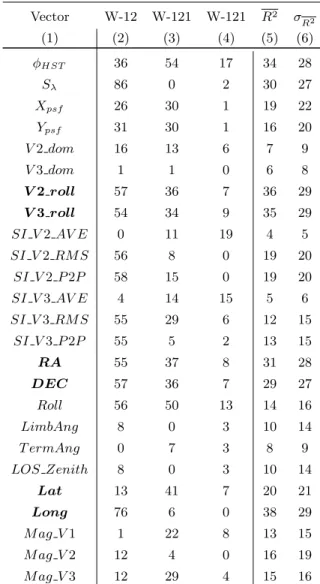
Table 1. Jitter engineering data optical state vectors (column 1) and the correlation R2 values (in %) with the white light curve photometry for the visits covering a STIS/G430L eclipse of 12 (column 1) and the STIS/E230M data of WASP-121 for visits 97 and visit 98 (columns 3 and 4 respectively). The average R2 value from 61 HST STIS G430L & G750L CCD visits, R2, is also reported in column 5, and the standard deviation of R2 in column 6. Vector W-12 W-121 W-121 R2 σ R2 (1) (2) (3) (4) (5) (6) φHST 36 54 17 34 28 Sλ 86 0 2 30 27 Xpsf 26 30 1 19 22 Ypsf 31 30 1 16 20 V 2 dom 16 13 6 7 9 V 3 dom 1 1 0 6 8 V 2 roll 57 36 7 36 29 V 3 roll 54 34 9 35 29 SI V 2 AV E 0 11 19 4 5 SI V 2 RM S 56 8 0 19 20 SI V 2 P 2P 58 15 0 19 20 SI V 3 AV E 4 14 15 5 6 SI V 3 RM S 55 29 6 12 15 SI V 3 P 2P 55 5 2 13 15 RA 55 37 8 31 28 DEC 57 36 7 29 27 Roll 56 50 13 14 16 LimbAng 8 0 3 10 14 T ermAng 0 7 3 8 9 LOS Zenith 8 0 3 10 14 Lat 13 41 7 20 21 Long 76 6 0 38 29 M ag V 1 1 22 8 13 15 M ag V 2 12 4 0 16 19 M ag V 3 12 29 4 15 16
Trends with telescope position are consistent with photometric systematics caused by slit light losses. If correct, the trends appear even when using slit sizes that are much greater than the size of the PSF. Our hypoth-esis is that the known telescope breathing leads to small changes in the position of the PSF on the detector (usu-ally at the sub-pixel level), which largely manifest them-selves as slit light losses. Even if the central PSF is well centered on a much wider slit, diffraction spikes and the
wide wings of the PSF could contribute to light losses. If the dominant source of systematics with STIS are po-sition related slit light losses, assuming similar guiding performance, then presumably there could be larger sys-tematics when using small slits such as the 0.200×0.200
used with the STIS E230M compared to the 5200×200slit
used with the CCD. In addition, there would be larger systematics in visits with poorer guiding performance, which appears to be the case. Several STIS visits in the PanCET program had guide star acquisition problems, which resulted in reduced pointing accuracy and light curves with comparably larger systematic trends. We also observe that the jitter vectors (V 2 roll, V 3 roll) and (RA and DEC) often have the same general trends as the traditional vectors (Sλ, Xpsf, and Ypsf), which
are measured directly from the spectra. Similar trends are generally expected, as changes in the PSF position (measured through the telescope position in the jitter files) will also be recorded by changes in the placement of the target stellar spectra on the detector. These vec-tors are not identical, however, as the detector-measured vectors will also be sensitive to further detector effects such as the pixel-to-pixel flat fielding, while the jitter vectors are able to record the telescope position regard-less of whether the target PSF is contained within the slit.
As a test, we implemented Jitter detrending on the STIS G430L eclipse data of WASP-12b, finding good agreement in the eclipse depth with Bell et al. (2017) who used a Gaussian process method to decorrelate the time series data (see AppendixA). However, several im-provements can be seen utilizing Jitter Detrending. The best-fit measured eclipse depth was found to be positive whileBell et al.(2017) found a negative value. In addi-tion, with Jitter Detrending the first orbit was success-fully recovered for use in the analysis, while Bell et al.
(2017) had to discard the orbit.
3. OBSERVATIONS
3.1. Hubble Space Telescope STIS NUV spectroscopy We observed two transits of WASP-121b with the HST STIS E230M echelle grating during 23 February 2017 (visit 97) and 10 April 2017 (visit 98). The ob-servations were conducted with the NUV-Multi-Anode Microchannel Array (NUV-MAMA) detector using the Echelle E230M STIS grating and a square 0.200×0.200
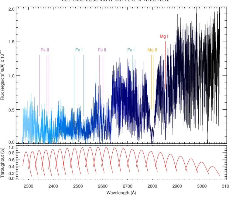
entrance aperture. The E230M spectra has resolving power of λ/(2∆λ) = 30,000 and was configured to the 2707 ˚A setting to cover the wavelength ranges between 2280 and 3070 ˚A in 23 orders (see Fig. 1). The result-ing spectra have a dispersion on the detector of approx-imately 0.049 ˚A/pix. Both transits covered five HST
Sing et al. spacecraft orbits, with the transit event occurring in the
third and fourth orbits. During each HST orbit, the spectra were obtained in TIME-TAG mode, where the position and detection time of every photon is recorded in an event list, which has 125 microsecond precisions.
We sub-divided the spectrum of each HST space-craft orbit into sub-exposures with the Pyraf task int-tag, each with a duration of 274.01996 seconds. This allowed orbits 2 through 5 to be divided into 10 sub-exposures each, while the first orbit was divided into 7 sub-exposures. These sub-exposures were then each re-duced with CALSTIS version 3.17, which includes the calibration steps of localization of the orders, optimal order extraction, wavelength calibration, and flat field corrections. The mid-time of each exposure was con-verted into BJDT DB for use in the transit light curves
(Eastman et al. 2010).
4. ANALYSIS
4.1. STIS E230M light curve fits
The light curves were modeled with the analytical transit models ofMandel & Agol(2002). For the white-light curves, the central transit time, planet-to-star ra-dius ratio, stellar baseline flux, and instrument sys-tematic trends were fit simultaneously, with flat pri-ors assumed. The inclination and stellar density (or equivalently the semi-major axis to stellar radius ratio, a/Rstar) were held fixed to the values found in Evans
et al.(2018), as fitting for these parameters found values
consistent with the literature, though with an order of magnitude lower precision. For example, we find a value of a/Rstar=3.63±0.16 from the NUV white light curve
of visit 98, whileEvans et al. (2018) reports a value of 3.86±0.02. Compared to the NUV data here, the study
ofEvans et al.(2018) benefits from much higher
photo-metric precision in a larger dataset with a wider array of wavelengths, including STIS data with complete phase coverage of the transit, which constrains the planet’s or-bital system parameters to a much greater degree than the NUV data alone.
The total parameterized model of the flux measure-ments over time, f (t), was modelled as a combination of the theoretical transit model, T (t, θ) (which depends upon the transit parameters θ), the total baseline flux detected from the star, F0, and the instrument
system-atics model S(x) giving,
f (t) = T (t, θ) × F0× S(x). (1)
Based on the results of section 2 and Appendix A, for our most complex systematics error model tested, we included a linear baseline time trend, φt, as well as the
traditional optical state vectors (φt, φHST, φ2HST, φ3HST,
φ4
HST, Xpsf, Ypsf & Sλ) and jitter vectors (V 2 roll,
V 3 roll, RA, DEC, Lat, & Long) resulting in up to fourteen total terms used to describe S(x) depending on the dataset in question as described below.
The errors on each datapoint were initially set to the pipeline values, which is dominated by photon noise. The best-fitting parameters were determined simultane-ously with a Levenberg-Marquardt (L-M) least-squares algorithm (Markwardt 2009) using the unbinned data. After the initial fits, the uncertainties for each data point were rescaled to match the standard deviation of the residuals. A further scaling was also applied to account for any measured systematic errors correlated in time (‘red noise’). After rescaling the error-bars, the light-curves were then refit, thus taking into account any un-derestimated errors in the data points.
The red noise was measured by checking whether the binned residuals followed a N−1/2 relation, when bin-ning in time by N points. In the presence of red noise, the variance can be modelled to follow a σ2= σ2
w/N +σ2r
relation, where σwis the uncorrelated white noise
com-ponent, and σr characterizes the red noise (Pont et al. 2006). For our best-fitting models for S(x), we did not find evidence for substantial rednoise.
The uncertainties on the fitted parameters were calcu-lated using the covariance matrix from the Levenberg-Marquardt algorithm, which assumes that the probabil-ity space around the best-fit solution is well-described by a multivariate Gaussian distribution. Previous anal-yses of other HST transit observations (Berta et al.
2012; Line et al. 2013a; Sing et al. 2013; Nikolov et al.
2014) have found this to be a good approximation when fitting HST STIS data. We also computed uncertain-ties with a Markov Chain Monte Carlo analysis (
East-man et al. 2013), which does not assume any functional
form for this probability distribution. In each case, we found equivalent results between the MCMC and the Levenberg-Marquardt algorithm for both the fitted pa-rameters and their uncertainties, as the posterior distri-butions were found to be Gaussian. Inspection of the 2D probability distributions from both methods indi-cate that there are no significant correlations between the systematic trend parameters and the planet-to-star radius contrast.
4.2. Limb darkening
The effects of stellar limb-darkening are strong at NUV wavelengths. To account for the effects of limb-darkening on the NUV transit light curve, we adopted the four parameter non-linear limb-darkening law, cal-culating the coefficients as described in Sing (2010). For the model, we used the 3D stellar model from
Figure 1. (Top) Flux calibrated out-of-transit spectrum of WASP-121A, each order is plotted in a different color. Several resonant lines of Mg and Fe are indicated. (Bottom) The instrumental throughput of each order.
the Stagger-grid (Magic et al. 2015) with the model (Tef f=6500, log g=4, [Fe/H]= 0.0), which was closest
to the measured values of WASP-121A in effective tem-perature, gravity, and metallicity (Tef f= 6460±140 K,
log10 g = 4.242±0.2 cgs, [Fe/H] = +0.13±0.09 dex;
Del-rez et al. 2016). The Stagger-grid 3D models are
calcu-lated at a resolution of R =20,000 which is close to the native resolution of the E230M data (R =30,000), and contains a fully line-blanketed NUV region that matches the flux-calibrated data of WASP-121A well (see Fig. 2). We included the individual responses from each order in the echelle spectra and converted the stellar model spec-tral wavelengths from air to vacuum. We also applied a wavelength shift to the data to take into account the systemic radial velocity of the system, 38.36 km/s (Gaia
Collaboration et al. 2018), shifting the star to the rest
frame.
In a test to see how well the 3D models performed, we fit visit 98 with a 3-parameter limb-darkening law
(see Sing 2010) and let the linear coefficient, c2, fit
freely while the other two non-linear parameters were fixed to the model values. We found good agreement at the 1-σ level between the fit coefficient c2=0.881±0.215
and the theoretical value of 1.077. In addition, the fit Rpl/Rstar= 0.1415 ± 0.0050 was also consistent (within
1-σ) when fitting for c2vs fixing the limb-darkening (see
Section4.4). For the remainder of the study, we fixed the limb-darkening coefficients to the model values. We note that using the second-order Akaike Information Crite-rion (AICc) for model selection (see AppendixA), that
Sing et al.
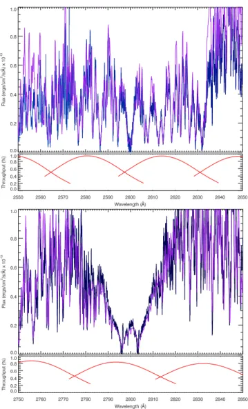
Figure 2. Same as 1, but zoomed in on two wavelength regions covering a Fe ii line at 2600 ˚A and the Mg ii doublet at 2796.35 and 2803.53 ˚A with the 3D Stagger-grid model overplotted (purple).
the AICc favoured fixing the limb-darkening parameters to the model values.
4.3. Updated ephemeris with NASA TESS data The Transiting Exoplanet Survey Satellite (TESS) ob-served WASP-121b in camera 3 from 7 Jan 2019 to 2 Feb 2019, and we obtained the timeseries photome-try though the Mikulski Archive for Space Telescopes’ exo.MAST2 web-service. We fit the TESS WASP-121b
transits using the Presearch Data Conditioning (PDC) light curve, which has been corrected for effects such as non-astrophysical variability and crowding (Jenkins
2https://exo.mast.stsci.edu
et al. 2016; Stumpe et al. 2012). From the timeseries,
we removed all of the points which were flagged with anomalies. The timeseries Barycentric TESS Julian Dates (BTJD) were converted to BJDTDB by adding
2,457,000 days. The TESS light curve contains data for 16 complete transits of WASP-121b and one par-tial transit. For each transit in the light curve, we extracted a 0.5 day window centered around the tran-sits and fit each transit event individually. We fit the data using the model as described in Sections 4.1
and 4.2, though only included a linear baseline time trend, φt, for S(x). We find a weighted-average value
of Rpl(TESS)/Rstar = 0.12342 ± 0.00015, which is in
good agreement with the HST transmission spectrum of
Evans et al.(2018). We converted the transit times of
Evans et al.(2018) and (Delrez et al. 2016) to BJDTDB
using the tools from (Eastman et al. 2010) and fit these along with the TESS transit times and visit 98 from Section 4.4 with a linear function of the period P and transit epoch E,
T (E) = T0+ EP. (2)
We find a period of P =1.2749247646 ± 0.0000000714 (days) and central transit time of T0= 2457599.551478
±0.000049 (BJDT DB). We find a very good fit with a
linear ephemeris (see Fig. 3), having a χ2 value of 16.8
for 21 degrees of freedom (DOF). We find no obvious signatures of quasi-periodic photometric variabiltiy due to stellar activity, with the TESS data binned by 62 minutes (excluding the transit and eclipse times) giving a standard deviation about the mean of 0.07% which is only modestly higher than the expected photometric precision of 0.02%.
4.4. White light curve fits
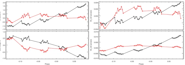
Visits 97 and 98 show dramatically different levels of instrumental systematic trends (see Fig. 4). In partic-ular, visit 97 shows a ∼4% change in flux in the 5th out-of-transit orbit, while for visit 98 there is no such large trend, and the light curve points are within ∼0.4% of each other. Upon inspection of the telescope RA and DEC from the jitter files, it is clear that visit 97 suf-fers from a very large drift during the 5-orbits covering the transit event, while visit 98 has much more stable pointing (see Fig. 5). The large drift likely leads to large slit light losses in visit 97. Most importantly, the RA and DEC positions of the telescope during the transit in visit 97 are significantly different than the out-of-transit positions, especially the 5th orbit that was shifted by about a quarter of a pixel. As discussed inGibson et al.
(2011), detrending with optical state vectors can only be expected to work if we interpolate the vectors for the
Figure 3. Observed - Calculated mid-transit times of WASP-121b. Included is the results fromDelrez et al.(2016) (dark green) andEvans et al.(2018) (blue) as well as the the NUV transit time (purple) and TESS times (grey) from this work. A zoom-in around the TESS mid-transit times is also shown. The 1-σ error envelope on the ephemeris is plotted as the horizontal dashed lines.
in-transit orbit(s), with the out-of-transit orbits, which requires the baseline function to be well represented by the linear model over the range of the decorrelation pa-rameters.
For each visit, we used the AICc and measured σr to
determine the optimal optical state vectors to include from the full set without overfitting the data while min-imizing the rednoise. As found in section 2, the differ-ent position related vectors from the Jitter files typically contained similar trends. For visit 98, we found it was optimal to include φHST terms up to a second order, as
well as the Jitter Detrending vectors V 2 roll, V 3 roll, and RA. We rotated the roll vector pair (V 2 roll, V 3 roll) which are contained in the engineering jitter files relative to the axis of the square slit (V n roll, V t roll), which is rotated by about 45 degrees relative to the spacecraft orientation reference vector U3, such that S(x) could be written as,
S(x) = p1φt+ p2φHST + p3φ2HST+
p4RA + p5V nroll+ p6V troll+ 1. (3)
The fit values of interest, namely Rpl/Rstar, did not
substantially change for any of the top fitting mod-els (AICc-AICcmin .6). With nine free parameters
(Rpl/Rstar, F0, T0, p1..6), the fit achieves a
signal-to-noise which is 81% of the theoretical photon signal-to-noise limit, with no detectable rednoise and a χ2
ν of 1.21 for 37
DOF. We note that including the jitter corrections and
Table 2. WASP-121b broad-band transmission spectral re-sults and non-linear limb darkening coefficients for the STIS E230M. λc ∆λ RP/R∗ σRP/R∗ c1 c2 c3 c4 ˚ A ˚A 2673 799 0.13735 0.00257 0.4011 -0.2625 1.2818 -0.4674 2387 236 0.15300 0.00845 0.4282 -0.8777 1.6772 -0.2513 2600 200 0.13962 0.00465 0.4826 -0.6976 1.9529 -0.7708 2800 200 0.13760 0.00366 0.4090 -0.2445 1.1797 -0.3940 2986 172 0.12734 0.00389 0.3374 0.2045 0.8312 -0.4348
the 2nd order breathing polynomial not only provides
a significantly better fit than the traditional systemat-ics model, but we were also able to make use of the first orbit in the visit. The overall photometric perfor-mance is similar to that achieved with the STIS CCD using the G430L or G750L, despite the use of a much narrower slit. With visit 97, we measure the white light curve Rpl/Rstar = 0.1374 ± 0.0026 (see Table 2)
and a T0 =2457854.536411±0.001073 (BJDT DB). The
central transit time agrees very well with the expected ephemeris, occurring -0.2±1.6 minutes relative to the ex-pected central transit time using the updated ephemeris from Section4.3.
For visit 97, even the most complex model did not achieve fit residuals as small as visit 98. As noted above, the fifth orbit of the visit displays dramatically increased systematic trends compared to the other orbits, with the position of the telescope during the orbit being relatively far from the position of the in-transit orbits (see Fig. 5). As such, we find the Rpl/Rstar can change dramatically
(by about 0.016 Rpl/Rstar) between differing
systemat-ics models when including the data from the fifth orbit in the light-curve fits. Given these factors, we find that it is preferable to drop the last orbit from the analysis when measuring the absolute transit depths in visit 97. This is similar to many HST STIS and WFC3 transit studies that have dropped the first orbit as it usually displays larger non-repeatable trends due to changes in the thermal breathing or charge trapping. When ex-cluding the fifth orbit, we found the fit Rpl/Rstarvalues
did not change substantially between differing system-atics models (∼0.008 Rpl/Rstar), and using the AICc,
we find S(x)=S(RA, V nroll, V troll, φt) to be optimal.
The best-fit planet radius for visit 97 is found to be Rpl/Rstar = 0.1364 ± 0.0110, which matches the value
from visit 98 at well within 1-σ, and achieves 43% of the theoretical photon noise limit.
Sing et al. 0.96 0.97 0.98 0.99 1.00 1.01 1.02
Normalised raw flux
1.01 1.02 0.97 0.98 0.99 1.00 Normalised flux Visit 97 Visit 98 -0.15 -0.10 -0.05 -0.00 0.05 -150 -100 -50 0 50 100 150 O-C ( × 10 -4) -0.15 -0.10 -0.05 -0.00 0.05 100 150
Planetary Orbital phase
Figure 4. WASP-121b E320M white light curves for visits 97 (left) and 98 (right). Top plot contains the raw flux, the middle panels contain the flux with the fitted instrument systematics model removed, and the bottom panel shows the residuals between the data and the best-fit model.
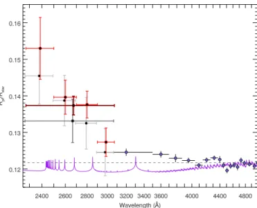
Figure 6. The STIS E230M NUV spectra of WASP-121b compared to the optical transmission spectrum. Plotted (red) is the broadband transmission spectra from visit 98 as well as the white light curve value (dark red). The broad-band spectra NUV spectra from visit 97 is also plotted (grey) along with the white light curve value (dark grey). The op-tical spectra are also shown (blue) along with a lower at-mospheric model fromEvans et al. (2018) covering ∼mbar pressures (purple) which was fit to the spectra long-ward of 4700 ˚A. The average optical to near-infrared (OIR) value of Rpl(OIR)/Rstar = 0.1217 is also shown by the dashed hori-zontal line.
When measuring the transmission spectrum, Rpl(λ)/Rstar,
we fixed the system parameters as they are not expected to have a wavelength dependence. In addition, we fixed the the limb darkening coefficients to those determined from the stellar model for each spectroscopic passband, using the same method as described in Section4.2. The light curve fitting methods were otherwise identical to those described in section4.1. We fit each spectroscopic light curve with the same functional systematics model as was found to optimally fit the white light curve, fit-ting the various spectroscopic bins simultaneously for the wavelength-dependent Rpl(λ)/Rstar and systematic
parameters p1..6.
Fig. 6 shows our resulting broadband spectra from visit 98 in ∼200 ˚A bins, as well as the NUV white light curve value. Rpl(λ)/Rstar is observed to sharply rise
toward shorter wavelengths. The overall NUV trans-mission spectrum shows strong extinction and is sub-stantially higher than the optical and near-IR, reach-ing altitudes of ∆Rpl(λ)/Rstar=0.0157±0.0026 higher in
the atmosphere. This is more than 18× the size of the pressure scale height of the lower planetary atmosphere, H = kT /µg, that is H/Rstar=0.00084 at a temperature
T of 2000 K.
While the overall transit depths of visit 97 are de-pendent upon the choice of S(x), the steep rise in the NUV broadband spectrum can be seen regardless of in-cluding or exin-cluding the fifth orbit from the analysis. When including the fifth orbit, a systematics model of S(x)=S(φHST, Sλ, RA, DEC, V nroll) produces a fit
radius that is both consistent with visit 98 and indepen-dent of excluding the fifth orbit. The resulting broad-band transmission spectra is shown in Fig. 6, which matches well with the results of visit 98.
Given the much lower precision and the sizeable sys-tematic uncertainty of including or excluding the fifth orbit in visit 97, we elect to report the transmission spec-tra at higher resolutions using visit 98 only. We fit the data to various resolutions and report the transmission spectra at a resolution of R ∼650, corresponding to 4 ˚
A bins with results from 5 ˚A bins also reported in Sec-tion 4.6. At these binsizes, each light curve point has a few thousand photons and the ∼1.5% transit depth can typically be detected across the E230M wavelength range. However, in the spectral regions with strong stel-lar absorption lines, or at the edges of the spectral or-ders where the efficiency is low, the transit itself is not always detected due to the lack of flux. At this res-olution, strong atomic transitions can be resolved and probed efficiently and a resolution-linked bias is min-imized (Deming & Sheppard 2017). Given the high resolution on the E230M, each 4 ˚A bin still contains ∼ 60 pixels. To help probe the central wavelength of the observed features more precisely, we also measured the transmission spectra in multiple 4 ˚A bin sets, each set shifted by 1 ˚A, corresponding to about 100 km/s ve-locity shifts (see Fig. 7). We removed points where the transit was not detected (Rpl(λ)/Rstar <0.05) or had
large errors (σRP/R∗ >0.09), which predominantly
oc-curred within strong stellar lines or at the order edges. The R∼650 NUV transmission spectrum can be seen in Figs. 8, 9,10, and11.
4.6. Mg i, Mg ii, Fe i and Fe ii
We find no evidence for absorption by Mg i. In a 5˚A band centered on the ground-state Mg i line at 2852.965 ˚
A, we measure a Rpl(Mg i)/Rstar=0.100±0.056, which
is consistent at the 1-σ confidence level with the optical and near-infrared value.
We find strong evidence for absorption by Mg ii. We detect and resolve absorption by both the k and h features of the Mg ii ground-state doublet located at 2796.35 and 2803.53 ˚A respectively (see Fig. 11). In 5 ˚A passbands, the transmission spectra in the Mg ii doublet is found to have radii of Rpl(Mg ii,k)/Rstar = 0.284 ±
Sing et al.
Figure 7. WASP-121b NUV transmission spectrum scanned in 4 ˚A passbands, with a 1 ˚A wavelength shift between each adjacent point. The data points have been colored with the significance in transit depth above/below that of the NUV broadband value, which is indicated by the dashed line at Rpl(NUV)/Rstar= 0.1374. The average optical to near-infrared (OIR) value of Rpl(OIR)/Rstar = 0.1217 is also shown by the solid black line.
substantially larger than the value at optical and near-IR (Onear-IR) wavelengths (Rpl(OIR)/Rstar = 0.1217) and
larger than the average NUV value of Rpl(NUV)/Rstar=
0.1374 ± 0.0026. A 10 ˚A passband split to cover the Mg ii doublet simultaneously is found to have a ra-dius value of Rpl(Mg ii,h,k)/Rstar = 0.271 ± 0.024 (see
Fig. 12), which is 5.4-σ above the white light curve Rpl(NUV)/Rstar value. In the continuum region
sur-rounding the Mg ii doublet, no other substantial absorp-tion features are observed and most all of the spectral bins in a 100 ˚A region around the doublet are consistent with the Rpl(OIR)/Rstar value (see Fig. 11).
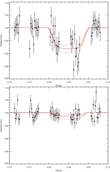
The strong Mg ii absorption can also be seen in the transit light curves, with Fig. 12showing transit depths of about 8% within the Mg line, while the surrounding continuum is consistent with the optical and near-IR transit depth of 1.5%. The stellar Mg ii double line cores exhibit narrow emission lines, associated with the stellar corona (see Fig. 2) with both peaks found just red-ward of the line centers at velocities near 20 to 40 km/s. We
performed several checks to ensure that the presence of the emission line did not adversely affect the planetary Mg ii signal. Inspecting the photometric time series of just the stellar Mg ii emission lines, we do not observe any substantial variability differences from that of the surrounding continuum. In addition, when scanning the transmission spectrum over the Mg ii region, we find the peak of the transmission spectrum is found 50 to 100 km/s blue-ward of the Mg ii line cores, rather than red-ward where the emission lines are located.
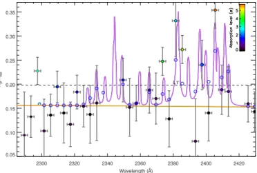
The transmission spectrum contains a very strong absorption feature at 2381.5 ˚A (Rpl(2381.5)/Rstar =
0.332 ± 0.074), which can be identified with a ground-state resonant transition of Fe ii. Fe ii transitions occur in a set of multiplets, with notable transitions at 2600, 2382, and 2344 ˚A for the UV1, UV2, and UV3 mul-tiplets respectively. For the aforementioned UV1 and UV3 ground-state transitions, the stellar line is strong enough such that almost no flux is measured in the line cores (see Fig. 2), so the transmission spectrum of the
Figure 8. WASP-121b NUV transmission spectrum in unique 4 ˚A passbands. The data points have been colored with the signif-icance in transit depth above that of the NUV spectra, which is indicated by the black dashed line at Rpl(NUV)/Rstar= 0.1374. A model fit that includes Fe i (green), Fe ii (purple) and Mg ii (orange) absorption is shown, with the complete model integrated over the spectral passband shown with (blue) open circles. The Lagrange point distance L10 is also indicated.
Figure 9. Same as 8 but zoomed in over the Fe ii UV2 region. Points have been removed in the spectral regions with strong stellar absorption lines, where the transit itself has not been detected due to low signal-to-noise.
planet can not be measured with sufficient precision at those wavelengths. However, other candidate Fe ii
fea-Figure 10. Same as 8 but zoomed in over the Fe ii UV1 region.
tures are also seen in the stellar spectrum (see Figs. 8,
9,10).
For Fe i, there are strong ground-state transitions in the NUV region at wavelengths of 2484, 2523, 2719,
Sing et al.
Figure 11. Same as8but zoomed in over the Mg ii region.
2913, and 2937 ˚A. While a significant absorption fea-ture does appear near 2484 ˚A (see Fig. 8), the other transitions of Fe i do not obviously appear in the data.
4.7. 1D Transmission Spectra Model
To help further identify absorption features, we fit a 1D analytic transmission spectral model to the data
(Lecavelier des Etangs et al. 2008), following the
proce-dures as detailed in Sing et al. (2015) and Sing(2018). Formally, the analytic model is isothermal and assumes a hydrostatic atmosphere with a constant surface grav-ity with altitude. These assumptions are not expected to be valid over the large altitude ranges probed by the NUV data, especially at very high altitudes. However, the model is useful for identifying spectral features in the transmission spectra, ruling out absorption by dif-ferent species, and getting a zeroth-order handle on the atmospheric properties, including the velocity. A more comprehensive and physically motivated modeling effort will be presented in a future work (P. Lavvas et al. in prep.).
To model the transmission spectra, a continuum slope was included, which was assumed to have cross sec-tion opacity with a power law of index α, (σ(λ) = σ0(λ/λo)−α). We also included the spectral lines of Mg i,
Mg ii, Fe i, and Fe ii with the wavelength-dependent cross-sections calculated using the NIST Atomic Spec-tra Database (Kramida et al. 2018). Voigt profiles were used to broaden the spectral lines. Given our trans-mission spectra are at very high altitudes, we did not include effects such as collisional broadening and choose instead to fit for the damping parameter governing the line broadening. We calculated the scale height assum-ing a mean molecular weight correspondassum-ing to atomic hydrogen and fit the model using an isothermal tem-perature. We also assumed that the number of atoms existing in the various atomic levels for a given species
Figure 12. Transit light curves for 10 ˚A wide passbands, which are corrected for systematic errors. (Top) A light curve composed of two 5˚A bins that are centered directly on the Mg II doublet, which optimally covers the two lines. (Bottom) A light-curve composed of two 5 ˚A bands placed adjacent to either side of the Mg II centered bands, which samples the nearby continuum. In both plots the average optical-near-IR radius is shown as the grey dashed lines. The red lines show the best-fit transit depths (solid) and the depths covering the 1-σ uncertanties (dashed).
followed a Boltzmann distribution with the statistical weights given in the NIST database, though this as-sumption may not be accurate at very low pressures. To simplify the calculation, we only included transitions where the lower energy level was beneath a threshold. High energy levels will in practice not be sufficiently populated to produce significant absorption signatures, and for Fe II we found transitions above 0.43 eV (cor-responding to 5000 Kelvin) were not prevalent in the data. However, the excited states of Fe II up to 0.43 eV
were needed, as including only ground-state transitions resulted in a much worse fit to the data. The presence of these excited states indicates high temperatures, as a significant population of Fe atoms are found above the ground state.
We fit the model to the NUV data with a L-M least-squares algorithm and MCMC (Eastman et al. 2013). The fit contained five free parameters: the isothermal temperature, α, the Doppler velocity of the planetary atmosphere, the reference planet radius, and the Mg and Fe abundances. We fit for the data between 2300 and 2900 ˚A, finding a good fit with a χ2 of 130.4 for 126
DOF. We estimate the detection significance of Fe ii by excluding its opacity from the model and refitting, find-ing the χ2increases by a ∆χ2=61.8, which corresponds
to a 7.9-σ detection significance. The velocity of the planetary atmospheric Mg and Fe lines is measured to be −56+43−63 km/s. Given the velocity uncertainties are larger than the spectrograph resolution, the uncertain-ties can likely be improved using different data reduction methods (e.g. smaller bins or using cross-correlation techniques), which will be presented in a future work (P. Lavvas et al. in prep.).
5. DISCUSSION
5.1. Constraints on the deep interior
A relatively cold planet interior can lead to the con-densing of refractory species deep in the atmosphere, thereby removing the gaseous species from the upper layers of the atmosphere, trapping them within conden-sate clouds at depth (Hubeny et al. 2003;Fortney et al.
2008; Powell et al. 2018), a process that is dependent
upon particle settling in the presence of turbulent and molecular diffusion (Spiegel et al. 2009;Koskinen et al. 2013). Al, Ti, VO, Fe, and Mg are among the first refrac-tory species to condense out of a hot Jupiter atmosphere
(Visscher et al. 2010; Wakeford et al. 2017). As such,
the presence or absence of these species can then provide constraints to the temperatures of the deeper layers for hot Jupiters, as the presence of these elements in the gas phase of the upper layers limits the global tempera-ture profile to be hotter than the condensation of these species. For WASP-121b, the NUV transmission spectra provides evidence for Mg and Fe in the exosphere, while the optical transmission spectrum shows signatures of VO but a lack of TiO (Evans et al. 2018). The presence of Fe can provide contraints on the interior temperature, Tint, as the element condenses at the highest
tempera-tures for pressures above about 100 bar (see Wakeford
et al. 2017).
We explore the constraints on the deep interior tem-perature (pressures ' 10 bar) using the best-fit retrieved
Figure 13. Temperature-Pressure profiles for WASP-121b (solid lines) compared to condensation curves computed for a metallicity of 10× solar (dashed lines). Interior temperatures from 100 to 500 K are shown.
temperature-pressure (T-P) profile for WASP-121b, de-rived from fitting the dayside emission spectra ofEvans
et al. (2017), which is sensitive to approximately bar
to mbar pressure levels and has recently been updated to include HST WFC3 G102 and Spitzer data (
Mikal-Evans et al. 2019). The T-P profile was generated
us-ing the analytical model of Guillot (2010), which as-sumes radiative equilibrium, and is parameterized with the Planck mean thermal infrared opacity, κIR, the
ra-tio of the optical to infrared opacity, γ, an irradiara-tion efficiency factor β, and the interior temperature of the planet, Tint. Emission spectra are not directly
sensi-tive to Tint (Line et al. 2013b), so retrievals often do
not probe the deep interior pressure layers and fix Tint,
withEvans et al.(2017) andMikal-Evans et al. (2019))
setting Tint to Jupiter-like 100 K values. However, with
both Mg and Fe present in the upper layers of the at-mosphere, temperatures of Tint=100 K are clearly too
low, as the T-P profile intersects Fe and Mg conden-sation curves at high pressures (see Fig. 13). As the condensation curves are metallicity dependent (Visscher
et al. 2010;Wakeford et al. 2017), we illustrate the
con-straints in Fig. 13 using 10× solar metallicity, which is close to the best-fit retrieved abundances for WASP-121b in both the transmission and emission spectrum
(Evans et al. 2018,2017, Evans et al. in prep). Varying
Tintin steps of 100 K and using the best-fit T-P profile
parameters [κIR=0.0049 cm2 g−1, γ=4.08, β=1.03], we
find internal temperatures near Tint=500 K are needed
to prevent both Fe and Mg from condensing deep in the atmosphere, but also allows TiO to condense at
pres-Sing et al. sures well below the photosphere. As discussed in
Fort-ney et al. (2008), for adiabatic interiors higher values
of Tint lead to warmer interiors and larger planet radii.
Given WASP-121b is one of the largest exoplanets found (Rpl= 1.865RJup,Delrez et al. 2016), a high Tint would
be expected. While there are computational limitations, we note that self-consistent 3D modeling efforts that in-clude both the deep interior and the exosphere in com-parison to transmission, emission and phase curve data can provide better constraints on the irradiation effi-ciency, atmospheric abundances, atmospheric mixing, and global T-P profiles, which in turn would provide the best condensation constraints on Tint.
5.2. Roche lobe geometry and exospheric constraints The ionized Mg and Fe lines are seen up to extremely high altitudes, corresponding to high planetary radii of Rpl/Rstar ∼0.3. We compare the altitudes of this
ab-sorption material to the theoretical distances of the L1 Lagrange point, DL1, and the L10 Lagrange point, DL10,
which is the distance between the planet’s center and the closest point of the equipotential surface including L1, which is the Roche lobe. Using the formalism inGu et al.
(2003) and using a mass ratio of Mpl/(Mpl+ Mstar) =
8.3 × 10⁻⁴ as well as a/Rstar = 3.76, we calculate
DL1/Rstar=0.24 (or 1.96Rpl) and the L10 Lagrange size
relative to that of the star to be DL10/Rstar=0.209 (or
1.72Rpl). In a transit configuration, the observed limit
of the Roche lobe is perpendicular to the planet-star direction and the Roche lobe extends to about 2/3 of the extension to the L1 Lagrange point (Vidal-Madjar
et al. 2008). For WASP-121b, we numerically calculated
the equivalent radius3of a transiting Roche lobe, R
eqRL,
finding ReqRL/Rstar = 0.158 (or 1.3 Rpl).
The core of the Mg ii k line reaches up to Rpl/Rstar=
0.309±0.036 (or 2.52±0.29Rpl), which is in excess
of ReqRL/Rstar at 4-σ confidence. In addition, the
ground-state Fe ii resonance line at 2382˚A reaches up to Rpl/Rstar =0.331±0.074 (or 2.7±0.6Rpl), which is in
excess of ReqRL/Rstar at 2.7-σ confidence. In a transit
configuration, these absorption features indicate that both Mg ii and Fe ii reach altitudes such that they are no longer gravitationally bound to the planet. While large hydrogen tails extending well beyond the Roche lobe have been seen at Lyman-α (Ehrenreich et al. 2015;
Bourrier et al. 2018), elements heavier than hydrogen in
exoplanets have not previously been found at distances in excess of the Roche lobe.
The existence of heavy atmospheric material reaching beyond the Roche lobe agrees with a geometric blow-off
3equivalent meaning the radius of a disk with the same area
scenario (Lecavelier des Etangs et al. 2004), where the Roche lobe is in close spatial proximity to the planet and the exobase can extend beyond it letting atmospheric gas freely stream away from the planet. WASP-121b is an ideal planet to potentially observe this phenomenon, as the planet is on the verge of tidal disruption (
Del-rez et al. 2016). At the terminator, the planet fills a
significant portion of it’s Roche lobe, with the optical-to-infrared radii reaching Rpl(OIR)/ReqRL=77%. The
NUV reaches Rpl(NUV)/ReqRL=87±2%, indicating the
NUV continuum contains opaque material nearly up to the transit-projected Roche lobe, while the cores of the Mg ii and Fe ii exceed the Roche lobe. A similar process is likely happening in comparably hot and tidally dis-torted planets such as WASP-12b, which also shows ev-idence of Mg ii and Fe ii absorption (Fossati et al. 2010;
Haswell et al. 2012). However WASP-121b has a more
favorable transmission spectral signal and orbits a signif-icantly brighter star than WASP-12A. These properties allow the WASP-121b NUV data to be fit at relatively high-resolution with a full limb-darkened instrument-systematic corrected transit model, which allows the transmission spectral line profiles to be well resolved and absolute transit depths preserved. Our transit light curves cover ingress, though no early ingress is observed as the NUV transit time is in excellent agreement with the expected ephemeris (see Section4.3). Like WASP-12b (Nichols et al. 2015; Turner et al. 2016), there is no evidence in WASP-121b for a bow-shock or mate-rial overflowing the L1 Lagrange point (Lai et al. 2010;
Vidotto et al. 2010; Llama et al. 2011; Bisikalo et al.
2013).
As ionized species, the Mg ii and Fe ii atoms are po-tentially sensitive to the planet’s magnetic field, which if strong enough could lead to magnetically controlled out-flows (Adams 2011). As such, departures in the transit light curves from spherical-symmetry and the velocity profile of the ionized lines could give insights into the nature of the outflow. Our data lacks complete phase coverage, so only has a limited ability to constrain a non-spherical absorption profile and we cannot constrain a possible post-transit cometary-like evaporation tail. However, we note that all of our transit light curve fits were well fit to near the photon-noise limit assuming the planet was a sphere. In addition, our model fit found ve-locities of −56+43−63 km/s, which does not have sufficient precision to confidently distinguish between outflowing blue-shifted gas or zero velocity gas.
6. CONCLUSION
We have presented HST NUV transit observations of WASP-121b and have introduced a new detrending
method, which we find helps improve the photometric performance of time-series HST STIS data. WASP-121b is one of the few exoplanets with a complete NUV-OIR transmission spectrum that can be compared on an ab-solute transit depth scale from NUV wavelengths into the near-IR. The whole NUV wavelength region shows significant absorption, with transit depths well in ex-cess of the optical and near-IR levels and a NUV con-tinuum that rises dramatically blueward of about 3000 ˚
A. We find spectral characteristics that have not previ-ously been observed, with strong features of ionized Mg and Fe lines that extend well above the Roche lobe ob-served, with multiple resolved spectral lines detected for both species. While not gravitationally bound, it is un-clear whether these ionized species are magnetically con-fined to the planet, though better signal-to-noise spec-tra would improve velocity measurements, and complete phase coverage searching for non-spherical symmetries could provide further insight. The presence of gas be-yond the Roche lobe is evidence this tidally distorted planet is undergoing hydrodynamic outflow with a geo-metric blow-off, where the exobase extends to or exceeds the Roche lobe, and elements heavier than hydrogen are free to escape. Spectrally resolved Mg ii and Fe ii fea-tures on an absolute transit depth scale will allow de-tailed simulations of the local physical conditions of the upper atmosphere, where it may be possible to deduce the altitude dependent density, temperature, and abun-dances of the upper atmosphere.
ACKNOWLEDGEMENTS
This work is based on observations made with the NASA/ESA Hubble Space Telescope that were obtained at the Space Telescope Science Institute, which is oper-ated by the Association of Universities for Research in Astronomy, Inc. Support for this work was provided by NASA through grants under the HST-GO-14767 pro-gram from the STScI A.G.M. acknowledges the sup-port of the DFG priority program SPP 1992 ”Explor-ing the Diversity of Extrasolar Planets (GA 2557/1-1). P.L. also acknowledges support by the Programme National de Plan´etologie (PNP) of CNRS/INSU, co-funded by CNES. L.B.-J. and P.L. acknowledge support from CNES (France) under project PACES. J.S.-F. ac-knowledges support from the Spanish MINECO grant AYA2016-79425-C3-2-P. This project has been carried out in part in the frame of the National Centre for Competence in Research PlanetS supported by the Swiss National Science Foundation (SNSF), and has received funding from the European Research Council (ERC) un-der the European Union’s Horizon 2020 research and innovation programme (project Four Aces; grant agree-ment No 724427). The authors would like to thank the staff at STScI for their extra efforts with these datasets which required special handling and scheduling. We also would like to thank the anonymous reviewer for their constructive comments and suggestions.
Facilities:
HST (STIS)Facilities:
TESSREFERENCES
Adams, F. C. 2011,ApJ, 730, 27
Ballester, G. E., & Ben-Jaffel, L. 2015,ApJ, 804, 116
Bell, T. J., Nikolov, N., Cowan, N. B., et al. 2017,ApJL, 847, L2
Ben-Jaffel, L. 2007,ApJL, 671, L61
—. 2008,ApJ, 688, 1352
Ben-Jaffel, L., & Ballester, G. E. 2013,A&A, 553, A52
—. 2014,ApJL, 785, L30
Berta, Z. K., Charbonneau, D., D´esert, J.-M., et al. 2012,
ApJ, 747, 35
Bevington, P. R., & Robinson, D. K. 2003, Data reduction and error analysis for the physical sciences (McGraw-Hill) Bisikalo, D., Kaygorodov, P., Ionov, D., et al. 2013,ApJ,
764, 19
Bourrier, V., Lecavelier des Etangs, A., Ehrenreich, D., et al. 2018,A&A, 620, A147
Brown, T. M., Charbonneau, D., Gilliland, R. L., Noyes, R. W., & Burrows, A. 2001,ApJ, 552, 699
Cauley, P. W., Shkolnik, E. L., Ilyin, I., et al. 2019,AJ, 157, 69
Delrez, L., Santerne, A., Almenara, J.-M., et al. 2016,
MNRAS, 458, 4025
Deming, D., & Sheppard, K. 2017,ApJL, 841, L3
Demory, B.-O., Ehrenreich, D., Queloz, D., et al. 2015,
MNRAS, 450, 2043
Eastman, J., Gaudi, B. S., & Agol, E. 2013,PASP, 125, 83
Eastman, J., Siverd, R., & Gaudi, B. S. 2010,PASP, 122, 935
Ehrenreich, D., Bourrier, V., Wheatley, P. J., et al. 2015,
Nature, 522, 459
Evans, T. M., Pont, F., Sing, D. K., et al. 2013,ApJL, 772, L16
Sing et al.
Evans, T. M., Sing, D. K., Wakeford, H. R., et al. 2016,
ApJ, 822, L4
Evans, T. M., Sing, D. K., Kataria, T., et al. 2017,Nature, 548, 58
Evans, T. M., Sing, D. K., Goyal, J. M., et al. 2018,AJ, 156, 283
Fortney, J. J., Lodders, K., Marley, M. S., & Freedman, R. S. 2008,ApJ, 678, 1419
Fossati, L., Ayres, T. R., Haswell, C. A., et al. 2013,ApJL, 766, L20
Fossati, L., Haswell, C. A., Froning, C. S., et al. 2010,
ApJL, 714, L222
Gaia Collaboration, Brown, A. G. A., Vallenari, A., et al. 2018,A&A, 616, A1
Garc´ıa Mu˜noz, A. 2007,Planet. Space Sci., 55, 1426
Gaudi, B. S., Stassun, K. G., Collins, K. A., et al. 2017,
Nature, 546, 514
Gibson, N. P. 2014,MNRAS, 445, 3401
Gibson, N. P., Nikolov, N., Sing, D. K., et al. 2017,
MNRAS, 467, 4591
Gibson, N. P., Pont, F., & Aigrain, S. 2011,MNRAS, 411, 2199
Gu, P.-G., Lin, D. N. C., & Bodenheimer, P. H. 2003,ApJ, 588, 509
Guillot, T. 2010,A&A, 520, A27
Haswell, C. A., Fossati, L., Ayres, T., et al. 2012,ApJ, 760, 79
Hoeijmakers, H. J., Ehrenreich, D., Heng, K., et al. 2018,
Nature, 560, 453
Hoeijmakers, H. J., Ehrenreich, D., Kitzmann, D., et al. 2019, arXiv e-prints,arXiv:1905.02096 [astro-ph.EP]
Hubeny, I., Burrows, A., & Sudarsky, D. 2003,ApJ, 594, 1011
Huitson, C. M., Sing, D. K., Pont, F., et al. 2013,MNRAS, 434, 3252
Jenkins, J. M., Twicken, J. D., McCauliff, S., et al. 2016,in Proc. SPIE, Vol. 9913, Software and Cyberinfrastructure for Astronomy IV, 99133E
Jensen, A. G., Cauley, P. W., Redfield, S., Cochran, W. D., & Endl, M. 2018,AJ, 156, 154
Koskinen, T. T., Yelle, R. V., Harris, M. J., & Lavvas, P. 2013,Icarus, 226, 1695
Kramida, A., Yu. Ralchenko, Reader, J., & and NIST ASD Team. 2018, NIST Atomic Spectra Database (ver. 5.6.1), [Online]. Available: https://physics.nist.gov/asd [2019, Feb 05]. National Institute of Standards and Technology, Gaithersburg, MD.
Lai, D., Helling, C., & van den Heuvel, E. P. J. 2010,ApJ, 721, 923
Lavie, B., Ehrenreich, D., Bourrier, V., et al. 2017,A&A, 605, L7
Lecavelier des Etangs, A., Pont, F., Vidal-Madjar, A., & Sing, D. 2008,A&A, 481, L83
Lecavelier des Etangs, A., Vidal-Madjar, A., McConnell, J. C., & H´ebrard, G. 2004,A&A, 418, L1
Lecavelier Des Etangs, A., Ehrenreich, D., Vidal-Madjar, A., et al. 2010,A&A, 514, A72
Lecavelier des Etangs, A., Bourrier, V., Wheatley, P. J., et al. 2012,A&A, 543, L4
Line, M. R., Knutson, H., Deming, D., Wilkins, A., & Desert, J.-M. 2013a,ApJ, 778, 183
Line, M. R., Wolf, A. S., Zhang, X., et al. 2013b,ApJ, 775, 137
Linsky, J. L., Yang, H., France, K., et al. 2010,ApJ, 717, 1291
Llama, J., Wood, K., Jardine, M., et al. 2011,MNRAS, 416, L41
Lothringer, J. D., Benneke, B., Crossfield, I. J. M., et al. 2018,AJ, 155, 66
Magic, Z., Chiavassa, A., Collet, R., & Asplund, M. 2015,
A&A, 573, A90
Mandel, K., & Agol, E. 2002,ApJ, 580, L171
Markwardt, C. B. 2009, in Astronomical Society of the Pacific Conference Series, ed. D. A. Bohlender, D. Durand, & P. Dowler, Vol. 411, 251
Mikal-Evans, T., Sing, D. K., Goyal, J., et al. 2019,
MNRAS, 1700
Murray-Clay, R. A., Chiang, E. I., & Murray, N. 2009,
ApJ, 693, 23
Nichols, J. D., Wynn, G. A., Goad, M., et al. 2015,ApJ, 803, 9
Nikolov, N., Sing, D. K., Pont, F., et al. 2014,MNRAS, 437, 46
Owen, J. E., & Jackson, A. P. 2012,MNRAS, 425, 2931
Pont, F., Zucker, S., & Queloz, D. 2006,MNRAS, 373, 231
Powell, D., Zhang, X., Gao, P., & Parmentier, V. 2018,
ApJ, 860, 18
Salz, M., Schneider, P. C., Fossati, L., et al. 2019, arXiv e-prints, arXiv:1901.10223
Sing, D. K. 2010,A&A, 510, A21
—. 2018, arXiv e-prints,arXiv:1804.07357 [astro-ph.EP]
Sing, D. K., Pont, F., Aigrain, S., et al. 2011,MNRAS, 416, 1443
Sing, D. K., Lecavelier des Etangs, A., Fortney, J. J., et al. 2013,MNRAS, 436, 2956
Sing, D. K., Wakeford, H. R., Showman, A. P., et al. 2015,
MNRAS, 446, 2428
Sing, D. K., Fortney, J. J., Nikolov, N., et al. 2016,Nature, 529, 59
Spiegel, D. S., Silverio, K., & Burrows, A. 2009,ApJ, 699, 1487
Stumpe, M. C., Smith, J. C., Van Cleve, J. E., et al. 2012,
PASP, 124, 985
Turner, J. D., Pearson, K. A., Biddle, L. I., et al. 2016,
MNRAS, 459, 789
Vidal-Madjar, A., Lecavelier des Etangs, A., D´esert, J.-M., et al. 2003,Nature, 422, 143
—. 2008,ApJL, 676, L57
Vidal-Madjar, A., D´esert, J.-M., Lecavelier des Etangs, A., et al. 2004,ApJL, 604, L69
Vidal-Madjar, A., Huitson, C. M., Bourrier, V., et al. 2013,
A&A, 560, A54
Vidotto, A. A., Jardine, M., & Helling, C. 2010,ApJL, 722, L168
Visscher, C., Lodders, K., & Fegley, Jr., B. 2010,ApJ, 716, 1060
Wakeford, H. R., Sing, D. K., Evans, T., Deming, D., & Mandell, A. 2016,ApJ, 819, 10
Wakeford, H. R., Visscher, C., Lewis, N. K., et al. 2017,
MNRAS, 464, 4247
Wakeford, H. R., Sing, D. K., Deming, D., et al. 2013,
MNRAS, 435, 3481
Yan, F., & Henning, T. 2018,Nature Astronomy, 2, 714
Sing et al.
Figure 14. White light curve of WASP-12b and selected jitter engineering measurements (V 3roll, V 3roll, RA, and DEC) for visit 3. Several traditional detrending variables (Xpsf, Ypsf and Sλ) are shown as well.
APPENDIX
A. BENCHMARKING JITTER DETRENDING WITH WASP-12B STIS CCD ECLIPSE DATA
We benchmarked the use of jitter detrending on the STIS G430L eclipse data of WASP-12b to verify the jitter engineering data could be used to detrend and fit STIS transit light curve data and to compare the performance with the latest methods. A subset of the optical state jitter vectors can be seen in Figure 14 for the 2017 June 15 STIS data. Results from these data have been published in Bell et al.(2017), who used a Gaussian process with the traditional model optical state vectors to model the light curve systematics. In our analysis, the data reduction steps were identical to Bell et al. (2017); however, we included the first HST orbit in our analysis and discarded the first exposure in each orbit.
We modelled N measured fluxes over time, f (t), as a combination of an eclipse model, T (t, δ) (which depends upon the eclipse parameter δ), the total baseline flux detected from the star, F0, and a parameterised systematics error
model S(x) giving,