HAL Id: hal-00305087
https://hal.archives-ouvertes.fr/hal-00305087
Submitted on 3 Aug 2007
HAL is a multi-disciplinary open access
archive for the deposit and dissemination of
sci-entific research documents, whether they are
pub-lished or not. The documents may come from
teaching and research institutions in France or
abroad, or from public or private research centers.
L’archive ouverte pluridisciplinaire HAL, est
destinée au dépôt et à la diffusion de documents
scientifiques de niveau recherche, publiés ou non,
émanant des établissements d’enseignement et de
recherche français ou étrangers, des laboratoires
publics ou privés.
for hydrologic applications: a review
S. P. Wechsler
To cite this version:
S. P. Wechsler. Uncertainties associated with digital elevation models for hydrologic applications: a
review. Hydrology and Earth System Sciences Discussions, European Geosciences Union, 2007, 11
(4), pp.1481-1500. �hal-00305087�
www.hydrol-earth-syst-sci.net/11/1481/2007/ © Author(s) 2007. This work is licensed under a Creative Commons License.
Earth System
Sciences
Uncertainties associated with digital elevation models for hydrologic
applications: a review
S. P. Wechsler
California State University Long Beach, 1250 Bellflower Boulevard, Long Beach CA 90840, USA Received: 24 April 2006 – Published in Hydrol. Earth Syst. Sci. Discuss.: 28 August 2006 Revised: 23 May 2007 – Accepted: 5 June 2007 – Published: 3 August 2007
Abstract. Digital elevation models (DEMs) represent the
to-pography that drives surface flow and are arguably one of the more important data sources for deriving variables used by numerous hydrologic models. A considerable amount of research has been conducted to address uncertainty associ-ated with error in digital elevation models (DEMs) and the propagation of error to derived terrain parameters. This re-view brings together a discussion of research in fundamen-tal topical areas related to DEM uncertainty that affect the use of DEMs for hydrologic applications. These areas in-clude: (a) DEM error; (b) topographic parameters frequently derived from DEMs and the associated algorithms used to de-rive these parameters; (c) the influence of DEM scale as im-posed by grid cell resolution; (d) DEM interpolation; and (e) terrain surface modification used to generate hydrologically-viable DEM surfaces. Each of these topical areas contributes to DEM uncertainty and may potentially influence results of distributed parameter hydrologic models that rely on DEMs for the derivation of input parameters. The current state of research on methods developed to quantify DEM uncertainty is reviewed. Based on this review, implications of DEM un-certainty and suggestions for the GIS research and user com-munities are offered.
1 Introduction
The purpose of this review is to examine the nature, relevance and management of digital elevation model (DEM) uncer-tainty in relation to hydrological applications. DEMs provide a model of the continuous representation of the earth’s ele-vation surface. This form of spatial data provides a model of reality that contains deviations from the truth, or errors. The nature and extent of these errors are often unknown and not
Correspondence to: S. P. Wechsler
readily available to users of spatial data. Our lack of knowl-edge about these errors constitutes uncertainty. Nevertheless, DEMs are one of the most important spatial data sources for digital hydrologic analyses as they describe the topography that drives surface flow. Use of DEMs in hydrologic stud-ies is ubiquitous, however uncertainty in the DEM represen-tation of terrain through elevation and derived topographic parameters is rarely accounted for by DEM users (Wechsler, 2003). DEM uncertainty is therefore of great importance to the hydrologic community.
This paper reports on representative literature on DEM un-certainty as applied to hydrologic analyses1. To understand how to address and manage DEM uncertainty, specifically in relation to hydrologic applications, it is necessary to recog-nize the components and characteristics of DEMs that con-tribute to that uncertainty. This paper provides a review of research in each of these fundamental areas which includes: (a) DEM error; (b) topographic parameters frequently rived from DEMs and the associated algorithms used to de-rive these parameters; (c) the influence of DEM scale as im-posed by grid cell resolution; (d) DEM interpolation; and (e) terrain surface modification used to generate hydrologically-viable DEM surfaces. Each of these topical areas contributes to DEM uncertainty and potentially influences results of dis-tributed parameter hydrologic models that rely on DEMs for the derivation of input parameters. The current state of re-search on methods developed to quantify DEM uncertainty is reviewed. Based on this review, implications of DEM un-certainty and suggestions for the research and GIS user com-munities are suggested.
In the past decade DEM data has become increasingly available to spatial data users due to the decrease in data and computer costs and the increase in computing power.
1Given the burgeoning nature of this literature, it regrettably has
not been possible to cite every publication on this topic. An attempt has been made to give examples of studies related to focal variables.
DEMs produced from technologies such as Light Detec-tion and Ranging (LiDAR) and Interferometric Synthetic Aperture Radar (IFSAR) sensors are more readily available. These remotely-sensed DEM production methods provide users with high resolution DEM data that have stated vertical and horizontal accuracies in centimeters, making them more desirable, yet costly in both dollars and processing require-ments. DEM users with limited budgets can obtain DEMs from government sources or can conduct field surveys using global positioning systems (GPS) and interpolate DEMs for smaller study areas. No matter the source, DEM products provide clear and detailed renditions of topography and ter-rain surfaces. These depictions can lure users into a false sense of security regarding the accuracy and precision of the data. Potential errors, and their effect on derived data and applications based on that data, are often far from users’ con-sideration (Wechsler, 2003).
In colloquial terms, the word error has a negative conno-tation, indicating a mistake that could have been avoided if enough caution had been taken (Taylor, 1997). However, er-rors are a fact of spatial data and often cannot be avoided. In the context of spatial data, errors are often unavoidable and therefore must be understood and accounted for. There has been much discussion in the literature regarding philoso-phies (Fisher, 2000), ontologies (Worboys, 2001) and defi-nitions (Heuvelink, 1998; Refsgaard et al., 2004) of spatial data uncertainty. For the purposes of this discussion of DEM uncertainty, the term error refers to the departure of a mea-surement from its true value. Uncertainty is a measure of what we do not know about this error and its impact on sub-sequent processing of the data. In the spatial realm, errors and resulting uncertainty can never be eliminated.
Our responsibilities as DEM data users and researchers are to accept, search for and recognize error, strive to understand its nature, minimize errors to the best of our technical capa-bilities, and obtain a reliable estimate of their nature and ex-tent. Based on these understandings, the tasks are to develop and implement methods to quantify and communicate the un-certainty associated with the propagation of errors in spatial data analyses. The research reported in this paper brings to-gether knowledge about the components and characteristics of DEM uncertainty specifically related to hydrologic appli-cations
2 DEM error and accuracy
2.1 DEM error
DEM errors (the departure of a given elevation from truth) have been well documented in the literature (Pike, 2002). DEM errors are generally categorized as either systematic, blunders or random (USGS, 1997). Systematic errors result from the procedures used in the DEM generation process and follow fixed patterns that can cause bias or artifacts in the
fi-nal DEM product. When the cause is known, systematic bias can be eliminated or reduced. Blunders are vertical errors associated with the data collection process and are generally identified and removed prior to release of the data. Random errors remain in the data after known blunders and systematic errors are removed.
Sources of DEM errors have been described in detail, see for example (Burrough, 1986; Heuvelink, 1998; Pike, 2002; Wise, 1998). Error sources have been summarized as (a) data
errors due to the age of data, incomplete density of
observa-tions or spatial sampling; (b) processing errors such as nu-merical errors in the computer, interpolation errors or clas-sification and generalization problems; and (c) measurement
errors such as positional inaccuracy (in the x and y
direc-tions), data entry faults, or observer bias.
2.2 DEM production methods and sources of error Sources of DEM errors are inextricably linked to DEM production methods. These include field surveying (using tacheometers or global positioning systems), photogramme-try, surface sensing technologies such as Light Detection and Ranging (LiDAR), Interferometric Synthetic Aperture Radar (IFSAR) or sonar (for bathymetric data), and digitizing from existing maps.
Errors are specific to the various production techniques. For example, the error budget for a LiDAR DEM is related to the contributing errors in data acquisition subsystems such as the laser rangefinder, global positioning system and inertial measurement unit (IMU) (Airborne1, 2006).
Once elevation data is collected, DEMs are generated us-ing interpolation or aggregation techniques. A detailed re-view of various interpolation approaches can be found in (Burrough and McDonnell, 1998; Burrough, 1986; Wood, 1996). Often little is known about the error either occurring during or generated as a result of the interpolation (Desmet, 1997) or aggregation process. Uncertainty associated with interpolation procedures has been a focus of practitioners and researchers in the geostatistical community (Dubois et al., 1998). However, relatively few studies explicitly address the impact that different interpolation methods have on a re-sulting DEM. A detailed review of various interpolation ap-proaches can be found in (Burrough and McDonnell, 1998; Burrough, 1986; Wood, 1996). The following are exam-ples of efforts to examine error that result from interpolation. Wood and Fisher (1993) and Wood (1996) applied visualiza-tion techniques to identify DEM interpolavisualiza-tion errors. Desmet (1997) investigated the effect of interpolation on precision (accuracy of the predicted heights) and shape reliability (de-gree of fidelity in the spatial pattern of topography) expressed by derived topographic parameters. Wise (1998) investigated the effect of interpolating DEMs from contours using differ-ent algorithms. Differences in results were attributed to the complex interactions between algorithms for both interpola-tion and derivainterpola-tion of DEM-derived topographic parameters
(Wise, 1998). Erxleben et al. (2002) evaluated the accu-racy of snow water equivalents derived from DEMs gener-ated using four interpolation methods. Kienzle (2004) tested the quality of DEMs interpolated at different resolutions and identified an optimum grid cell size that was determined to be between 5–20 m depending on terrain complexity. These studies reveal the variety of applications that are affected by DEM error and the efforts of researchers to document and to accommodate for error.
2.3 Quantifying DEM error
In the United States, national map accuracy standards pro-vide statistical guidelines for estimating the positional accu-racy of digital geospatial data (FGDC, 1998). DEM vendors establish threshold accuracies for specific products based on technological capabilities. DEM accuracy is quantified us-ing the Root Mean Square Error (RMSE) statistic. To com-pute the RMSE, differences between the source dataset and co-located values from an independent source of higher ac-curacy are computed. The RMSE is the square root of the average of these squared differences.
The RMSE assumes that DEM errors are random (FGDC, 1998). Because the RMSE is used as a measure of spread, it requires the assumption of normality (Monckton, 1994), which is often violated in the case of the DEM. While a valu-able quality control statistic, the RMSE does not provide an accurate assessment of how well each cell in a DEM repre-sents a true elevation.
The following example demonstrates the limitations of the RMSE. A LiDAR dataset that consists of roughly 120 million points has a stated vertical accuracy (RMSE) of 0.15 m. This value was computed from an external ground survey of 174 co-located points (representing 0.00014% of the dataset). A normal distribution with a mean of 0 and a standard devia-tion of 0.15 could range from −0.62 to +0.62. The vendor assures 95% of the data could deviate from the stated eleva-tion by 0.15 m or less. However, five percent of the values (six million points) could deviate by ±0.15 to ±0.30 m and 1% (1.2 million points) by ±0.30 to ±0.62 m. The RMSE’s adequacy in representation of the dataset’s accuracy is ques-tionable.
Maune (2001) provides a detailed review of DEM pro-duction methods and associated quality assessment. This includes source, size and spatial structure of error associ-ated with different DEM production techniques. Examples of studies that have evaluated the accuracy of various DEM products are: DEMs produced from synthetic aperture radar (SAR) (Wang and Trinder, 1999), the Shuttle Radar Topogra-phy Mission (SRTM) (Miliaresis and Paraschou, 2005; Suna et al., 2003), USGS DEMs (Berry et al., 2000; Shan et al., 2003), and comparisons of various DEM production methods (Li, 1994). While methods to assess and reduce DEM error have been developed (Hengl et al., 2004; Li, 1991; Lopez, 2002), errors persist. The inability to specify the relative
con-tribution of these errors and quantify their nature and extent in a DEM product results in uncertainty.
Assessment of DEM uncertainty requires more informa-tion on the spatial structure of DEM error – beyond that provided by the RMSE. DEM vendors have been urged to provide additional DEM quality information such as “maps
of local probabilities for over or underestimation of the un-known reference elevation values from those reported in the DEM, and joint probability values attached to different spa-tial features” (Kyriakidis et al., 1999, p. 677). DEM data
products should not only include information on standard er-rors associated with data values, but also provide values for error contributed by other sources, such as components of the production methods, so that DEM error can be correctly assessed (Heuvelink et al., 2007).
To date, information beyond the RMSE is not readily pro-vided to DEM users. Most DEM users will not take the time or spend the money to obtain such data sets in order to con-duct DEM error assessment (Wechsler, 2003). Because in-formation on sources of error are not readily available, it is currently often difficult, if not impossible, to recreate the spa-tial structure of error for a particular DEM. As demonstrated in the example above, quality control data points represent only a small percentage of a dataset and are insufficient to quantify the spatial structure of the DEM’s error. Knowledge about the spatial structure of error is an important compo-nent for gaining an understanding of where errors arise and uncertainty is propagated. DEM vendors should be urged to provide information that can be used to derive this and DEM users must be able to easily apply such information for it to be of use. Therefore the research and software communities should develop DEM assessment methods that accommodate detailed DEM error information when available, and provide mechanisms for addressing uncertainty in the absence of this information.
3 Computation of topographic parameters for hydro-logic analyses
Topographic attributes frequently used in hydrologic analy-ses are derived directly from DEMs. DEM errors propagate to derived parameters. While numerous algorithms exist to generate these hydrologic parameters, GIS software pack-ages limit users’ ability to select specific algorithms. Addi-tionally, the hydrologic community has not reached a consen-sus on appropriate algorithms for certain topographic param-eters (such as flow direction). This section discusses the cal-culation of certain topographic parameters from DEMs and identifies considerations related to their contribution to un-certainty in hydrologic applications.
The raster grid structure lends itself well to neighborhood calculations that are frequently used to derive hydrologic pa-rameters directly from a DEM. Primary surface derivatives such as slope, aspect and curvature provide the basis for
characterization of landform (Evans, 1998; Wilson and Gal-lant, 2000). The routing of water over a surface is closely tied to surface form. Flow direction is derived from slope and aspect. From flow direction, the upslope area that con-tributes flow to a cell can be calculated, and from these maps, drainage networks, ridges and watershed boundaries can be identified. Topographic, stream power radiation and tem-perature indices are all secondary attributes computed from DEM data. Wilson and Gallant (2000) provide a detailed review of the DEM-derived primary and secondary topo-graphic attributes. Research has demonstrated that DEM-derived topographic parameters are sensitive to both the qual-ity of the DEMs from which they are generated (Bolstad and Stowe, 1994; Wise, 2000) and the algorithms that are used to produce them.
Numerous algorithms exist for calculating topographic pa-rameters. For example, slope is calculated for the center cell of a 3×3 matrix from values in the surrounding eight cells. Algorithms differ in the way the surrounding values are selected to compute change in elevation (Carter, 1990; Dunn and Hickey, 1998; Guth, 1995; Hickey, 2001; Skid-more, 1989). Different algorithms produce different results for the same derived parameter and their suitability in repre-senting slope in varied terrain types may differ. The slope algorithm developed by Horn (1981) and currently imple-mented in ESRI GIS products is thought to be better suited for rough surfaces (Burrough and McDonnell, 1998; Horn, 1981). The slope algorithm presented by Zevenbergen and Thorne (1987), currently implemented in the IDRISI GIS package (Eastman, 1992), is thought to perform better in rep-resenting slope on smoother surfaces (Burrough and McDon-nell, 1998; Zevenbergen and Thorne, 1987).
The routing of flow over a surface is an integral compo-nent for the derivation of subsequent topographic parameters such as watershed boundaries, and channel networks. Many different algorithms have been developed to compute flow direction from gridded DEM data and are referred to as sin-gle or multiple flow path algorithms. The sinsin-gle flow path method computes flow direction based on the direction of steepest descent in one of the 8 directions from a center cell of a 3×3 window (Jenson and Domingue, 1988), a method referred to as D8. The D8 algorithm is the flow direction algorithm that is provided within mainstream GIS software packages (such as ESRI GIS). However, the users in the hy-drologic community recognize that the D8 approach over-simplifies the flow process and is insufficient in its character-ization of flow from grid cells. In response, researchers have developed multiple flow path methods that distribute flow in all possible down-slope directions, rather than just one; see for example (Costa-Cabral and Burgess, 1994; Quinn et al., 1991; Tarboton, 1997; Wolock and McCabe, 1995; Zhou and Liu, 2002). Multiple flow path methods attempt to approxi-mate flow on the sub-grid scale. Multiple flow path functions are currently not part of standard GIS packages and are there-fore not readily available to DEM users. Desmet and Govers
(1996) compared six flow routing algorithms and determined that single and multiple flow path algorithms produce signif-icantly different results. Thus any analysis of contributing areas such as watersheds or stream networks can be greatly affected by the algorithm implemented. Other approaches to deriving channel networks and watershed boundaries have been developed such as those that incorporate additional en-vironmental characteristics (Vogt et al., 2003).
Unfortunately, GIS packages do not differentiate between rough and smooth surfaces when applying a slope or provide users with any options when it comes to derivation of terrain parameters. Users cannot choose a particular method; only one algorithm for derivation of parameters such as slope, as-pect and flow direction is embedded in a particular GIS soft-ware package. This lack of flexibility in softsoft-ware capability introduces the likelihood of further error transferred to de-rived topographic parameters. Additional research on the ap-propriateness of certain algorithms for various terrain types is needed. Future GIS software packages should accom-modate research needs by providing flexibility in the algo-rithms available to users. The ability to represent topographic complexity is controlled by the DEM’s grid cell resolution. Systematic errors are introduced into topographic parame-ters, specifically slope, computed in flat areas and (Wechsler, 2000) and slopes computed for the same DEM but using a higher grid cell resolution results in larger computed slope values.
4 DEM resolution and scale for representing topography
Theobald (1989) noted that “. . . seldom are errors described
in terms of their spatial domain, or how the resolution of the model interacts with the relief variability.” (p. 99). This
continues to be a concern for users.
The raster GIS grid cell data structure makes it possible to represent locations as highly defined discrete areas. The size of a grid cell is commonly referred to as the grid cell’s resolution, with a smaller grid cell indicating a higher resolu-tion. DEM accuracy has been shown to decrease with coarser resolutions which average elevation within the support (Li, 1992). Smaller grid cell sizes allow better representation of complex topography. These high resolution DEMs are bet-ter able to refine characbet-teristics of complex topography that are missed in coarser DEMs. This has led many DEM users to seek the highest DEM resolutions possible, increasing the costs associated with both data acquisition and processing. However, is higher resolution necessarily better? To what extent is the grid cell resolution a factor in the propagation of errors from DEMs to derived terrain parameters? Studies have addressed these questions.
DEM-derived data is generated to emulate or predict a pro-cess. The scales of environmental processes are often un-known because they occur at a range of scales. Topography
is a result of many different processes operating over a range of spatial and temporal scales. DEM resolution imposes pro-cess and measurement scales on topography and thus hydro-logic analyses. Scale questions must be addressed to fully understand earth processes, and how these processes are re-flected in the geographic pattern and form of the landscape (Quattrochi and Goodchild, 1997).
DEM resolution has been shown to impact a wide range of hydrologic derivatives. These include: flow direction (Usul and Pasaogullari, 2004), topographic index (Quinn et al., 1991; Quinn et al., 1995; Rodhe and Seibert, 1999; Valeo and Moin, 2000), drainage properties such as chan-nel networks and flow extracted from DEMs (Garbrecht and Martz, 1994; Lacroix et al., 2002; Tang et al., 2001; Wang and Yin, 1998). Other hydrologic applications have been impacted including the spatial prediction of soil attributes (Thompson et al., 2001), computation of geomorphic mea-sures such as area-slope relationships, cumulative area dis-tribution and Strahler stream orders (Hancock, 2005), mod-eling processing of erosion and sedimentation (Schoorl et al., 2000), computation of soil water content (Kuo et al., 1999), slope and specific catchment area as applied to land-slide modeling (Claessens et al., 2005) and output from the popular rainfall-runoff model TOPMODEL (Brasington and Richards, 1998; Saulnier et al., 1997). DEM resolution has also been shown to directly impact hydrologic model pre-dictions from TOPMODEL (Band and Moore, 1995; Quinn et al., 1995; Wolock and Price, 1994; Zhang and Mont-gomery, 1994), the SWAT model (Chaplot, 2005; Chaubey et al., 2005), and the Agricultural Nonpoint Source Pollution (AGNPS) (Perlitsh, 1994; Vieux and Needham, 1993). The Water Erosion Prediction Project (WEPP) model, however, was not sensitive to coarser resolution DEMs unless the res-olution compromised watershed delineation (Chochrane and Flanagan, 2005).
The impact of grid cell resolution on terrain parameters has been shown to be related to both topographic complexity and the nature of the algorithms used to compute terrain at-tributes. For example, a variety of algorithms have been used to compute slope from grid-DEMs using various grid cell res-olutions. In each case, as the DEM resolution became finer the calculated maximum slope became larger (Armstrong and Martz, 2003; Bolstad and Stowe, 1994; Carter, 1990; Chang and Tsai, 1991; Gao, 1997; Jenson, 1991; Toutin, 2002; Yin and Wang, 1999). Larger slope values in higher resolution DEMs can specifically be attributed to the nature of the slope algorithm, in which the grid cell resolution is effectively the “run” in the rise-over-run formula.
Research to determine an appropriate grid cell resolution for particular analyses has been undertaken (Albani et al., 2004; Kienzle, 2004). The literature has established that the grid cell size of a raster DEM significantly affects derived terrain attributes (Kienzle, 2004). Research has also demon-strated that higher resolution is not necessarily better when it comes to the computation of DEM derived topographic
parameters (Wechsler, 2000; Zhou and Liu, 2004) and con-tributes to the propagation of errors to derived parameters under uncertain conditions (Wechsler, 2000). Selection of an appropriate resolution ultimately depends on characteristics of the study area such as topographic complexity, nature of the analysis, and finances available to purchase high resolu-tion DEM data if appropriate.
The repeated outcomes of the effects of grid cell resolution in various hydrologic applications suggest that grid cell res-olution will remain an important factor in our understanding, assessment and quantification of the propagation of DEM er-rors to hydrologic parameters and resulting uncertainty in re-lated modeling applications.
Variability at scales larger than those captured by the grid cell area, referred to as sub-grid variability, exists, but has for the most part, been ignored. To date, sub-grid information is either unavailable or lost through interpolation techniques. However, as technologies progress and more and more data becomes available from DEM production methods (such as LiDAR which produces millions of data points used for DEM interpolation), sub-grid information could be retained. Meth-ods to differentiate data from noise will need to be developed. This additional information could become a useful compo-nent for future DEM uncertainty estimations. Modifications to the raster grid cell structure should allow larger grid cells for representation of flatter areas and smaller grid cells for areas of topographic complexity, all within the same DEM. This coupled with appropriate algorithms for varied topog-raphy may lead to more appropriate representation of terrain surfaces for hydrologic applications.
5 Surface modification for hydrologic analyses
Overland flow routing through grid cells of a DEM requires a DEM without disruptions. DEMs often contain depressions that result in areas described as having no drainage, referred to as sinks or pits. These depressions disrupt the drainage sur-face, which preclude routing of flow over the surface. Sinks arise when neighboring cells of higher elevation surround a cell, or when two cells flow into each other resulting in a flow loop, or the inability for flow to exit a cell and be routed through the grid (Burrough and McDonnell, 1998; ESRI, 1998). Hydrologic parameters derived from DEMs, such as flow accumulation, flow direction and upslope contributing area, require that sinks be removed. This has become an ac-cepted and common practice.
To use a DEM as a data source in hydrologic analyses, sinks must be removed, a “necessary evil” according to Bur-rough and McDonnell (1998) and Rieger (1998). Sinks, how-ever, can be real components of the surface. For example in large scale data where surface hummocks and hollows are of importance to surface drainage flow, sinks are accurate fea-tures. With the advent of high resolution (submeter grid cell) DEMs it is likely that sink filling operations will be costly not
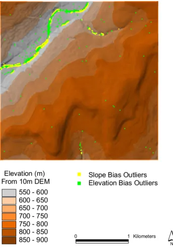
% % % % %% % % % %% % % % % % % % % % % % % % % % % %% % % %%%%%% %%%%%%% % % %%%%%%%%%%%%%%%%%%%%%%%%%%%%%%%%%%%%%%%%%%%%%%%%%%%%%%%%%%%%%%%%%%%%%%%%%%%%%%%%%%%%%%%%%%%%%%%%%%%%% %%% %%%%%%%%%%%%%%%%%%%%%%%% %%%%%%%% % %%%%%%%%%%%%%% %%%%%% % %%%%%%%%%%%%%%%% %%%%%%% %%%%%%%%%%%%%%%%%%%%%%%%%%%%%%%%%%%%%%%%%%%%%%%%%%%%%%%%%%%%%%%%%%%%%%%%%%%%%%%%%%%%%%%%%%%%%%%%%%%%%%%%%%%%%%%%%%%%%%%%%%%%%%%%%%%%%%%%%%%%%%%%%%%%%%%%%%%%%%%%%%%%%%%%%%%%%%%%%%%%%%% %%%%%%%%%%%%%%%%%%%%%%%%%%%%%%% %%%%%%%%%% %%%%%%%%%%%%%%%%%%%%%%%%%%%%%%%%%%%%%%%%%%%%%%%%%%%%%%%%%%%%%%%%%%%%%%%%%%%%%%%%%%%%%%%%%%%%%%%%%%%%%%%% %%%% %%%%%%%%% %%%%%%%%%%%%%% %%%%%%%%%%%%%%%% %%%%%%%%%%% %%%%%%%%%%%%%%%%%%% % %%%%%% %%%%%%%% % %%%%%%%% %%%%%%%%%%%%%%%%%%%%%%%%% %%%%%%% %%%%%%%%%%%%%%%%%%%%%%%%%%%%%%%%%%%%%%%%%%%%%%%%%%%%%%%%%%%%%%%%%%%%%%%%% % %%%%%%%%%% % %% % %%%%% % % % % %%%%%% %% % %%%%%%%%%%%%%%%%% %%%%%%%%%%%%% %%%%%%% %%%%%%%%%%%%%%%%%%%%%%%%% % %%%%%% %%%%%%%%%%%%%%%%%%%%%%%%%%%%%%%% %%%%%%% %%%%% %%%% %%% %%%%%%%% % %%%%%%%%%%%% %%%%% %%%%%%%%%%%% %%%% %%%%%%%% %%%%% %%%%%%%%%% %%%% %%% %%%%%%%%%%%%%%% % % %%%%%%%%%%%%%%%% % % % %%% % %%%%%%%%% %%% %%%%%%% % % % % %% % %%%%%%%%%%%%%%%%%%%%% %%%%%%%%%%%%%%%%%% %%%%%%%%%%%% %%%%%%%%%%%%%%%%%%%% 0 1 Kilometers
Locations of Bias Due To Sink Filling
Subsection of Claryville, NY Quadrangle
N Elevation (m) From 10m DEM 550 - 600 600 - 650 650 - 700 700 - 750 750 - 800 800 - 850 850 - 900 %
Elevation Bias Outliers Slope Bias Outliers
%
Fig. 1. Topographic locations of bias outlier points due to sink
fill-ing. Points contributing to positive elevation bias and negative slope bias were extracted from results of a Monte Carlo Simulation (ele-vation bias values greater than 1.61 and slope bias values less than
−3.78). Locations tend to coincide, falling in valley areas or loca-tions with relatively flat slopes.
only in processing time, but in removing naturally occurring features of the terrain surface.
Naturally occurring sinks in elevation data with a grid cell size of 100 m2or larger are rare, although they could occur in glaciated or karst topography (Mark, 1988; Tarboton et al., 1993). Rodhe and Seibert (1999) treated depressions in a 50×50 m grid as real topographic features as part of a process to identify mires. However, generally sinks are often treated as artifacts of the DEM creation method and eliminated.
Sinks are identified by simply identifying impediments to a flow direction surface derived from a DEM. A number of methods have been described for distinguishing (Lind-say and Creed, 2006) and eliminating depressions in DEMs (Hutchinson, 1989; Jenson, 1991; Jenson and Domingue, 1988; Lindsay and Creed, 2005a; Martz and Garbrecht, 1999; O’Callaghan and Mark, 1984; Rieger, 1998).
Methods to determine whether a sink is actual, or an arti-fact of the DEM are time intensive. They include (a) ground inspection through field survey, (b) examination of the source data used to generate the DEM, (c) development of a clas-sification model for a particular DEM that can be used to train the computer to recognize depressions in a particular data source, (d) knowledge-based approaches that incorpo-rate heuristic rules specific to a data set (Lindsay and Creed, 2006).
Methods used to eliminate depressions include: (a) sink
filling which raises elevations in the DEM to match
sur-rounding cells so that flow paths can be routed, (b)
breach-ing which lower cell elevations along a breach to route flow
and (c) combinations of these approaches that both raise and lower grid cells (Lindsay and Creed, 2005a). Although an evaluation of four different methods (Lindsay and Creed, 2005a) suggests that the breaching method and a combi-nation method are better alternatives (Lindsay and Creed, 2005a), the sink filling approach is the one most commonly found integrated into mainstream GIS software.
Sink filling is based on the D8 single flow direction flow routing method first described by Jenson and Domingue (1988) and Jenson (1991). This approach raises the sink ele-vation to that which enables flow linkage. The method has the disadvantage of assuming that all depressions are due to an underestimation of elevation in the sink, rather than the overestimation of surrounding cells, and flow routing is based on the D8 single-direction flow algorithm discussed previously. Other algorithms have been developed that incor-porate the multiple flow path approach (Martz and Garbrecht, 1999; Rieger, 1998).
While research has focused on the development of sink filling methods, little attention has been paid to either the ap-propriateness of a particular sink filling algorithm or to the impact of the sink filling operation on DEMs and derived pa-rameters. Wechsler (2000) investigated the impact of DEM errors and the sink filling procedure on representation of el-evation and derived parameters using a Monte Carlo simula-tion technique. The effect of sink filling was quantified di-rectly for elevation and slope and indidi-rectly for the TI. While there was no significant difference between elevation from filled and unfilled DEMs, a significant bias was observed in the slope parameter. The sink filling procedure raised the ele-vation of cells where sinks were found, increasing eleele-vations in these areas, resulting in a larger positive bias for elevation. Raising these elevations in turn decreased slope estimators in these areas, leading to negative bias for slope (Fig. 1). These findings have implications for watershed studies conducted in lower lying, flatter areas such as agricultural watersheds. Lindsay and Creed (2005) also evaluated the impact of de-pression filling on DEMs and derived topographic parame-ters and similarly concluded that depression removal signif-icantly alters the spatial and statistical distributions of de-rived terrain attributes. The occurrence of depressions in re-motely sensed DEMs representing varying terrain types (flat
to mountainous) was evaluated. As would be expected, flat areas experienced more depressions than high-relief land-scapes. The number of depressions found was related to grid cell resolution; coarser grids were found to be more vulnera-ble to depressions (Lindsay and Creed, 2005b).
In addition to the process of sink filling, hydrologists fre-quently undertake a method of surface modification referred to as stream burning, to generate “hydrologically enforced” DEMs (Maune, 2001). The method integrates vector repre-sentation of hydrography with the interpolation of the DEM. This automatic adjustment of the DEM has been incorporated into the ANUDEM package (Hengl et al., 2004; Hutchinson, 2006). The impact of this surface modification procedure on derived parameters has not been addressed in the litera-ture. An advantage of this procedure is that it avoids iterative modification of the entire DEM, focusing on just the low ly-ing stream areas. Errors could result from inconsistencies between the data sources, specifically in regard to scale.
DEMs are altered to generate surfaces over which flow can be routed to facilitate their use in further hydrologic analyses. The impact of this modification on resulting analyses bears further investigation.
6 Distributed parameter hydrologic models
“GIS do not ‘create’ information. However there appears to have developed an implicit reliance on GIS to provide information adequate to parameterize physically based dis-tributed hydrological models, often at spatial resolution and accuracy levels that are unrealistic given the original source of spatial data.” (Band and Moore, 1995, p. 419)
GISs are designed to represent environmental features, such as topography, which drive dynamic hydrologic (and other environmental) processes. Although they are not de-signed to serve as dynamic modeling tools (Reitsma and Albrecht, 2005) the ability of the GIS to represent the dis-tributed nature of data sets lends itself well as a platform for integrating distributed hydrologic models.
Topography is the driving force behind the hydrologic re-sponse of a watershed. Hydrologic processes are represented by and analyzed using hydrologic models. Many hydrologic models are distributed in nature; terrain representation is di-vided into smaller areas or grid cells within which hydrologic processes are simulated. The raster grid structure allows flow to be routed through the watershed via grid cells. This struc-ture integrates well with distributed parameter hydrologic models that are designed to accept grid-based inputs such as derived topographic parameters. Grid-based DEMs have been used ubiquitously to generate input parameters such as slope gradient, aspect, curvature, flow direction and upslope contributing area, for distributed parameter hydrologic mod-els (Armstrong and Martz, 2003; Johnson and Miller, 1997; Saghafian et al., 2000).
The use of a GIS to generate input parameters for dis-tributed parameter models enables a watershed to be
ana-lyzed at higher resolutions than would be practical using manual methods. The distributing of hydrologic informa-tion imposes an inherent scale on hydrologic analyses that must be recognized. The effect of this scale is often not ac-knowledged and the results of the effects of this scale are neither quantified nor considered when presenting results from various hydrologic models. Sensitivity analyses are frequently performed by hydrologists on model inputs such as hydrograph estimations, and Manning’s roughness coeffi-cients. However, they are rarely performed on DEM-derived attributes such as slope, aspect and flow direction. This leads to a number of questions such as: What is the appropriate
grid cell resolution for a hydrologic analysis? How does un-certainty propagate from the DEM to input parameters and through the models?
As discussed above, outputs from distributed parameter hydrologic models such as WEPP, SWAT, AGNPS and Top-Model have been shown to be highly sensitive to grid cell size. Lagacherie et al. (1996) evaluated the propagation of error in topographic parameters through a hydrologic model to simulate flood events. Variations in outputs were docu-mented and were not linear. Differences in DEM vertical ac-curacies were shown to impact the accuracy of runoff predic-tions from the soil-hydrology-vegetation model (DHSVM) (Kenward et al., 2000).
Hydrologic models are complex. Identifying sources of error in DEMs is difficult enough. Understanding their prop-agation to topographic parameters compounds the problem. The Generalized Likelihood Uncertainty Estimation (GLUE) method provides a mechanism for estimating uncertainty in hydrologic model predictions (Beven and Binley, 1992) and has been applied to assess uncertainty in TopModel which requires a DEM to derive input parameters (Freer et al., 1996). However, understanding, quantification and commu-nication of how errors in numerous input parameters often required of physically-based hydrologic models affect their output continues to challenge (Beven, 2006; Beven and Bin-ley, 1992). Practitioners often undertake hydrologic analy-ses with a hope that error propagation to hydrologic param-eters is minimal when combined within hydrologic models. A clear cut answer is preferred over the concept of equifi-nality (Beven, 2006; Beven, 2007). However, is it safe to make this assumption without assessing or reporting the un-certainties associated with input parameters, especially those derived from DEMs? Research has indicated that even small discrepancies can have a meaningful impact on the results of hydrologic models, and could influence the way hydrologic information, as represented by hydrologic models is evalu-ated and interpreted. Users of hydrologic models must be aware of the influence that both the DEM and GIS software have on the calculation of various model parameters. The task ahead is to develop accepted methodologies for quanti-fying and communicating propagation of DEM errors to re-sults of hydrologic analyses.
7 DEM uncertainty simulation
DEM error and issues of specific consideration for their use in hydrologic analyses have been identified in the preceding sections. This section reviews theories associated with spa-tial data uncertainty and their application, and reviews how the research community has responded to quantify and rep-resent DEM uncertainty.
7.1 Stochastic simulation
The “simulation school” (Chrisman, 1989) regards the map as a distribution of possible realizations within which the true values lie. Given spatial data uncertainty, a DEM can be garded as only one rendering of a distribution of possible re-alizations. The stochastic simulation approach to error mod-eling requires a number of maps, or realizations, upon which selected statistics are performed. Uncertainty is computed by evaluating the statistics associated with the range of outputs. Representation of these equiprobable distributions of maps is referred to as stochastic modeling (Chrisman, 1989; Journel, 1996), or Monte Carlo simulation due to the random genera-tion of uncertain variables used to simulate uncertainty.
Monte Carlo simulation assumes that the DEM is only one realization of a host of potential realizations. Each cell there-fore can be represented by a probability distribution func-tion (PDF) and each cell has a known mean and variance. A value is drawn from the PDF for each cell. This pro-cess repeated many times generating a set of realization maps (Burrough and McDonnell, 1998). In Monte Carlo analyses the outcomes represent the entire space by generating a com-plete probability distribution of possible outcomes (Srivasta, 1996).
Stochastic simulations provide a series of random plau-sible maps using stochastic modeling methods from mathe-matical statistics. The technique does not ensure that a “real” map is generated from the process (Chrisman, 1989), but the simulation does provide a bound within which we can state the true map lies. Simulation techniques can therefore be used to represent uncertainty about the true elevation.
Much research has focused on the use of simulation techniques to propagate error and quantify uncertainty in spatial data (see for example Brunsdon and Openshaw (1993), Deutsch and Journel (1998), Goodchild et al. (1992), Heuvelink et al. (1989), Openshaw et al. (1991), Veregin (1994)). Alternatives to Monte Carlo simulation include an-alytical models of error propagation based on Taylor Series expansion (see for example Albani et al. (2004), Bachmann and Allgower (2002), Heuvelink (1998), and Heuvelink et al. (1989)). However, Monte Carlo simulation is the ap-proach commonly applied to assess DEM uncertainty regard-ing error propagation “. . . Monte Carlo methods have almost
completely taken over. . . ” (Heuvelink et al., 2007, p. 91).
This can be attributed to their relative simplicity in concept, advances in computing power that have facilitated the
com-putational demands of this brute force approach, and the “simplifying approximations” required of analytical methods in the face of complexity (Heuvelink et al., 2007). For the purposes of this review, selected examples of methods based on the Monte Carlo simulation approach are presented. 7.2 Representing DEM errors by random fields
The differences among Monte Carlo methods for simulating DEM uncertainty lie in the methods used to generate
ran-dom fields. A ranran-dom field2 is a surface of random values that estimates the magnitude, variance and spatial variability of uncertainty. Each value represents the potential error at a specific point (grid cell). These error maps represent the PDF of the DEM’s error distribution, which accounts for the magnitude and spatial dependence of DEM error. Realiza-tions derived from these random fields are used to quantify DEM uncertainty. The value of each cell in a random field represents one possible case from a PDF that is developed to describe what is know about a DEM’s error.
The Monte Carlo simulation approach, as applied to DEMs, can be summarized as follows. a) A random field (error map) is generated based on statistical representation selected for DEM error. b) The random field is added to the original DEM resulting in a realization. c) Steps a. and b. are repeated N times based on the number of realizations deemed appropriate to capture the distribution of possible elevations. d) The distribution of these realizations is evaluated and un-certainty is quantified. Multiple realizations of the DEM pro-vide a Gaussian distribution that better represents the DEM under uncertain conditions (Fisher, 1998; Hunter and Good-child, 1997).
The underlying assumptions of the Monte Carlo simula-tion procedure as applied to DEM uncertainty assessment are as follows: (a) DEM error exists and constitutes uncer-tainty that is propagated with manipulation of the elevation data; (b) The nature and extent of these errors is unknown; c) DEM error can be represented by a distribution of DEM realizations; and d) The true elevation lies somewhere within this distribution (Wechsler, 2000; Lindsay, 2006).
Approaches to random field generation are based on two different assumptions: (a) No prior knowledge of the spa-tial structure of DEM error is available. Higher accuracy data can be difficult and costly to obtain. In the absence of this information, random fields can be approximated by the accuracy statistic (RMSE) provided with DEM metadata, and methods to incorporate spatial autocorrelation within
2The random function model for estimating uncertainty is rooted
in the field of geostatistics and is based on an assumption of local stationarity which assumes that spatial properties are independent of location. Error is complex and is likely non-stationary, and spatially autocorrelated. The assumption of stationarity, however, applies to the search neighborhood, not the entire data set and as such is a “viable assumption even in data sets for which global stationarity is clearly inappropriate” (Isaaks and Srivasta, 1989, p. 532).
these fields. (b) The second assumption is the empirical ap-proaches which assume that the spatial structure of DEM error is available. This information can be obtained from higher accuracy data generated from ground truth surveys or other DEMs and can be integrated into random field genera-tion.
7.3 Estimating the parameters of random fields
A number of methods have been presented for representing uncertainty through random fields. Simple uncorrelated ran-dom fields are normally distributed with a mean of 0 and a standard deviation often equivalent to the RMSE, which is typically the only information DEM users have about a DEM’s accuracy (Hunter and Goodchild, 1997; Van Niel et al., 2004; Wechsler, 2000; Wechsler and Kroll, 2006). How-ever, Tobler’s First Law of Geography – everything is related
to everything else, but near things are more related than dis-tant things – cannot be ignored (Tobler, 1970). The
uncorre-lated representation of error fields as “worst case scenarios” was refuted by Oksanen (2006). Elevation is characterized by spatial dependence, or autocorrelation, therefore eleva-tion errors are spatially autocorrelated. The nature of this autocorrelation is difficult to assess due to the complexity as-sociated with DEM errors and potential anisotropic nature of error. However, the following methods have been developed to account for spatial autocorrelation in random fields.
Spatial moving averages apply a filter to the random field
to increase its spatial autocorrelation. These filters range from 3×3 low pass filters to those that account for the dis-tance of spatial dependence as computed by a semivariogram of the original DEM (Liu and Herrington, 1993; Wechsler and Kroll, 2006).
A process referred to as pixel swapping (Fisher, 1991; Goodchild, 1980) is based on the geostatistical concept of
simulated annealing (Deutsch and Journel, 1998; Oksanen,
2006). A threshold spatial autocorrelation is identified based on properties of the input data. The spatial autocorrelation of the random field is computed. Two cells in the field are ran-domly identified, values in the two cells are swapped and the spatial autocorrelation recalculated. The steps are repeated until the difference between the threshold and calculated au-tocorrelation is within a certain threshold.
A spatial autoregressive model was presented by Hunter and Goodchild (1997). Error fields were generated using a spatially dependent disturbance term based on a spatially au-toregressive process: e=We+N (0, 1), where e represents a vector of grid values of the disturbance field, is a parameter, and N (0,1) is a vector of normally distributed random num-bers (mean of 0, standard deviation of 1). W is a matrix of weights that assigns a 1 to rook’s case neighbors, and 0 other-wise. This forces to lie in the range of 0 to 0.25 (Hunter and Goodchild, 1997). The disturbance maps were simulated it-eratively selecting values of e and fitting them to the equation
until the equation worked. Distinct patterns of autocorrela-tion emerged as reached values close to 0.25.
Sequential Gaussian simulation is a geostatistical
ap-proach that assumes errors are normally distributed and their distribution can be approximated by using higher accuracy data obtained from ground control points (Aerts et al., 2003). Random fields are generated as follows: each node in the grid is visited randomly. At each node original observations and simulated nodes are selected for conditioning and krig-ing is used to obtain descriptive statistics of this conditional cumulative distribution function (CCDF). A random value is drawn from the CCDF and placed in that node location. The process is repeated until all locations have been populated (Journel, 1996; Oksanen, 2006).
Additional methods that require data beyond the RMSE to establish the spatial structure of DEM error have been in-troduced. Elschlaeger (1998) developed a method that re-quires higher accuracy data derived from a GPS survey or higher resolution DEM to inform the development of the random field (Ehlschlaeger, 1998; Ehlschlaeger and Short-ridge, 1996; Holmes et al., 2000). This
three-parameter-method creates random fields with a Gaussian distribution
that matches the mean and standard deviation parameters de-rived from a “difference map”. Spatial autocorrelative char-acteristics of spatially dependent uncertainty are accounted for in the algorithm. This method improves upon the pixel swapping and spatial autoregressive approaches which allow only one parameter to define the structure of the error model (Ehlschlaeger, 1998; Oksanen, 2006).
Kyriakidis et al. (1999) present a geostatistical method that is based on a combination of sparsely available higher accuracy (“hard” data) with given DEM elevations (“soft” data). Elevation realizations are generated by cokriging and are based on auto- and cross-covariance models that quantify the autocorrelation and cross-correlation between the hard and soft data (Kyriakidis et al., 1999; Oksanen, 2006) . 7.4 DEM Error Simulation: Case Studies
“...there is no inherent reason why conditional simulation should not be used as routinely for uncertainty analysis as kriging is used for interpolation. It is unlikely, how-ever, that conditional simulation will become available in the GIS environment until a substantial demand has been estab-lished...this is likely to require the gradual accumulation of case studies in the literature...” (Englund, 1993 p. 437).
Each of the following case studies demonstrates the ap-plicability of the Monte Carlo simulation approach to er-ror propagation and uncertainty assessment in DEMs and DEM-derived data. These studies establish that progress has been made in demonstrating the applicability and effec-tiveness of these approaches to error propagation within a Monte Carlo Simulation. However the varied error prop-agation approaches indicate that an agreed approach is as of yet unresolved. The remaining challenge is to provide
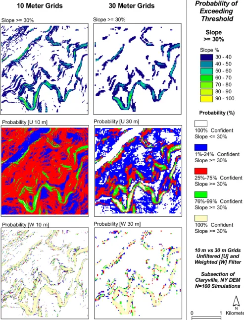
Probability [W 30 m] Probability [W 10 m] Probability [U 10 m] Probability [U 30 m] Slope >= 30% Slope >= 30% 30 Meter Grids 10 Meter Grids Slope % 30 - 40 40 - 50 50 - 60 60 - 70 70 - 80 80 - 90 90 - 100 0 1 Kilometers N 10 m vs 30 m Grids
Unfiltered [U] and Weighted [W] Filter Subsection of Claryville, NY DEM N=100 Simulations Probability of Exceeding Threshold Slope >= 30% 1%-24% Confident Slope >= 30% 25%-75% Confident Slope >= 30% 76%-99% Confident Slope >= 30% 100% Confident Slope <= 30% 100% Confident Slope >= 30% Probability (%)
Fig. 2. Results of a Monte Carlo simulation demonstrating the probability that slopes will be >=30%. Two methods for generating
ran-dom fields were used: U corresponds to uncorrelated ranran-dom fields and W represents spatially autocorrelated ranran-dom fields. The results demonstrate the effects of uncertainty using two different random field methods and grid cell resolutions (10 and 30 m).
these approaches as tools that DEM users can readily ac-cess through GIS software packages. There will be occa-sions when a DEM user has access to a higher accuracy data source for generating information on the spatial structure of error, and there will be occasions when that information is unavailable.
7.4.1 Higher accuracy data unavailable
The following studies incorporate either the RMSE statistic for a particular DEM or expert judgment regarding develop-ment of the error fields.
The Pixel swapping algorithm presented by Goodchild (1980) has been applied in a number of studies. Lee et al. (1992) found that floodplain delineations were signifi-cantly affected by DEM error. Fisher (1993) simulated the impact of DEM error on viewshed analyses using this method and determined that DEM-derived viewsheds may overesti-mate representation of the “true” viewshed. Davis and Keller (1997) modified the Goodchild (1980) approach to model un-certainty in slope stability prediction. The modified method was used to increase spatial autocorrelation in error field gen-erated by variogram analyses. The authors suggested that this method could be improved by incorporating autocorrelation
at different levels of aggregation based on slope classes, user defined windows or slopes. The Goodchild (1980) method was also adapted by Veregin (1997) to incorporate slope in the iterative swapping approach. In this approach, slope served as an underlying indicator of the spatial distribution of DEM error. Flow paths derived from DEMS using the D8 method were found to be sensitive to DEM errors, especially in areas of low slope. Murillo and Hunter (1997) applied the spatially autocorrelation iterative swapping method to evalu-ate the effect of DEM error on prediction of areas susceptible to landslides. While uncertainty associated with some model input such as choice of slope classes and slope algorithms were acknowledged the impact of these uncertainties was not assessed. Uncertainty results were communicated through visualization via map output. Lindsay (2006) applied this approach to assess the impact of DEM error on six meth-ods for extracting channel networks from a DEM. Methmeth-ods that required identification of patterns from surface morphol-ogy (valley-recognition algorithms) were more sensitive than channel-initiation techniques, perhaps because elevation er-ror was shown to influence positioning of channel heads and links (Lindsay, 2006).
Hunter and Goodchild (1997) applied a spatially autore-gressive random field method that incorporates spatial auto-correlation of DEM error. This method was compared with completely random, uncorrelated error fields to assess the ef-fect of these error representations on slope and aspect calcu-lations. The authors concluded that an error model ought to be based on an assumption of spatial dependence of error; however, completely random fields could be applied in the absence of a higher accuracy surface from which to obtain this information.
Wechsler (2000) and Wechsler and Kroll (2006) compared simulations resulting from four different methods of random fields that included completely random (mean of 0 and stan-dard deviation equal to the RMSE) and three different filter methods that increased the spatial autocorrelation of the error fields. Wechsler (2000) applied this method to evaluate the effects of DEM uncertainty on sink filling, topographic pa-rameters calculated at different resolutions, and topographic parameters computed for different terrain types (Figs. 2 and 3). Although less sophisticated than the iterative swapping method to achieving spatial autocorrelation, the methodol-ogy was implemented directly via an extension to a com-monly used GIS software package.
Widayati et al. (2004) implemented the error propagation methods presented by Wechsler (2000) to evaluate the prop-agation of elevation error on flat and varied slopes and dif-fering grid resolutions. Slope error was found to be sensitive to the spatial dependence of DEM error. Cowell and Zeng (2003) assessed uncertainty in the prediction of coastal haz-ards due to climate change. Uncertainty in the DEM was rep-resented by random, normally distributed error fields. As er-ror was increased, model output uncertainty decreased due to the nature of the normal distribution of the error fields used.
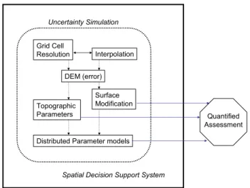
Uncertainty Simulation DEM (error) Topographic Parameters Grid Cell Resolution Interpolation Surface Modification
Distributed Parameter models
Spatial Decision Support System
Quantified Assessment
Fig. 3. Spatial model of a DEM uncertainty SDSS toolbox.
Yilmaz et al. (2004) simulated DEM error using completely random fields with a normal distribution based on the RMSE to demonstrate the impact of DEM uncertainty on the results of a flood inundation model.
More recently, a “process convolution” or spatial moving averages approach to the generation of random error fields was used to evaluate the delineation of drainage basins that were found to be very sensitive to DEM uncertainty (Oksa-nen and Sarjakoski, 2005a; Oksa(Oksa-nen and Sarjakoski, 2006). The approach was applied to both slope and aspect deriva-tives and demonstrated that completely random uncorrelated random error fields are not a valid mechanism for represent-ing DEM error (Oksanen and Sarjakoski, 2005b; Oksanen and Sarjakoski, 2006).
Methods for assessing DEM uncertainty through simula-tion and error propagasimula-tion have not been fully integrated into assessing hydrologic model output with the exception of Zerger (2002) who investigated the effect of DEM uncer-tainty on a storm surge model. Random error fields were spatially autocorrelated. DEM errors impacted low inunda-tion scenarios. This spatial uncertainty was communicated using visualization through risk maps.
7.4.2 Higher accuracy data available
Another school of thought on error propagation assumes that the RMSE alone is an insufficient indicator of DEM error, and that additional knowledge of the spatial structure of error in a particular DEM is required for uncertainty modeling in a Monte Carlo simulation. Approaches have been developed that incorporate higher accuracy data, such as that garnered from a higher accuracy DEM or GPS survey, to develop a model of the spatial structure of error, which in turn is used to generate DEM realizations.
Ehlschlaeger and Shortridge (1996) developed a model that creates random fields with a Gaussian distribution that
matches the mean and standard deviation derived from a higher accuracy data source. Spatial autocorrelative charac-teristics of spatially dependent uncertainty are accounted for in the algorithm that was applied to a least-cost-path appli-cation. Kiriakidis et al. (1999) present a geostatistical ap-proach to DEM realizations that incorporate autocorrelation information derived from residuals obtained from higher ac-curacy sources. Holmes et al. (2000) applied this approach to the prediction of slope failure. Endreny and Wood (2001) evaluated the effect of DEM error on flow dispersal area pre-dictions using six different algorithms. Error fields were spa-tially autocorrelated based on an error matrix derived from an assessment of differences between the test USGS 30 m DEM and a higher resolution 10m SPOT DEM. Uncertainty results were communicated using probability maps. Ehlschlaeger (2002) introduced a method for generating error fields that accounts for both the spatial autocorrelation of error and in-corporates information about DEM characteristics such as topological shapes in the error model. Canters et al. (2002) evaluated the effects of DEM error on a landscape classifica-tion model. Random error fields were spatially correlated us-ing error characteristics derived from a ground truth survey. While uncertainty caused by image classification was found to be more significant than DEM error, transition zones were particularly sensitive to DEM error. Van Niel et al. (2004) ap-plied Monte Carlo simulation to assess the impact of DEM uncertainty on slope, aspect, net solar radiation, topographic position and topographic index. The error in these DEM-derived parameters was propagated to results of a vegetation model. DEM error was assessed by comparison with a higher accuracy data source obtained from a GPS survey and used to filter normally distributed random error fields.
8 Integrating and communicating DEM uncertainty
“. . . The absence of facilities within GIS software for han-dling the effects of input data uncertainty and possible error propagation by GIS operations creates a question mark over the safe utilization of many aspects of the technology. . . ”
(Openshaw et al., 1991, p. 78)
Methods have been developed that transfer information from a GIS into external error propagation analysis tools (see for example Heuvelink (1998), Hwang et al. (1998)). Output from these external systems is either returned to the GIS for mapping and visualization or exported to graphic charts or statistical tables (Hwang et al., 1998). Attempts have also been made to integrate uncertainty simulation tools within a GIS (Wechsler, 2000). However, a viable DEM uncertainty
toolbox that incorporates various simulation approaches, and
considers the fundamental areas that contribute to DEM un-certainty described herein has not yet been realized. What are the essential components of a viable DEM uncertainty
tool-box and what form should it take? How should simulation
results be quantified and communicated?
8.1 User interfaces: decision support systems
Assessment of the multiple factors that contribute to DEM uncertainty and their propagation to topographic parameters and hydrologic models is complex. The ability of a user to interact with and explore possible outcomes is crucial for in-formed decision making. Spatial decision support systems (SDSS) provide a mechanism for integrating data exploration and assessing model outcome to facilitate informed decision making and can serve as a mechanism for achieving this interaction with DEM users. An SDSS is generally com-prised of a spatial database and a user-defined interface that accesses GIS analysis and modeling capabilities. Multiple Criteria Decision Models (MCDM) are a type of SDSS that allow users to make decisions with multiple alternatives (As-cough et al., 2002; Jankowski et al., 2001).
Current GIS interfaces provide limited support for spa-tial data exploration and uncertainty assessment. However, many GIS user interfaces can now be modified and enhanced through object-oriented programming that allows users to de-velop tools to assess model results and assist in decision mak-ing based on these results. Such direct integration of deci-sion support tools that incorporate uncertainty theory within a GIS has been achieved on a limited basis. Wechsler (2000) and Wechsler and Kroll (2006) integrated a toolbox within a GIS to allow users to simulate the effects of DEM error on elevation, slope, upslope area and the topographic in-dex. While results were not carried through to a particular hydrologic modeling effort, and used simple error propaga-tion techniques, the approach demonstrated how these tools can be integrated as pull-down-menus into mainstream GIS. Aerts et al. (2003) developed an SDSS external to a GIS to assess the impact of DEM uncertainty on a cost-path anal-ysis for ski run development. Although uncertainty associ-ated with specific model input parameters such as slope can-not be culled out, and the product is can-not specifically part of a GIS package, the research successfully demonstrates the efficacy of such an approach. Gunther (2003) developed a software program called SLOPEMAP, that integrates with two commonly used terrain analysis packages (ArcView GIS and Surfer) to derive geologic information from a DEM for assessment of rockslide susceptibility. Debruin and deWit (2005) developed a method to streamline the evaluation of grids within a stochastic simulation. This computer applica-tion demonstrates progress in the use of Monte Carlo simu-lations on desktop computers. Currently some GIS packages have limitations on the number of grids that can be assessed simultaneously. Other GIS-based decision support tools have been developed. Wise et al. (2001) report on the results of the successful integration of a GIS-based user interface for statistical spatial data analysis. Dura˜nona and Lopez (2000) developed a toolbar to detect errors in a DEM. Crosetto and Tarantola (2001) present general procedures for assess-ment of uncertainty within a GIS-based flood forecasting model. Karssenberg and DeJong (2005) describe concepts
for integrating error propagation functionality based on ex-isting concepts within an environmental modeling language. They concede that a consistent framework for implementing error propagation into environmental modeling has not been achieved and suggest that this is because tools are not avail-able or accessible for a wide range of users (Karssenberg and Jong, 2005).
Each of these studies demonstrates the viability of the SDSS as a mechanism for addressing DEM uncertainty, and integrating that knowledge with specific distributed parame-ter hydrologic models. There is as of yet no consensus about how to present these tools and to communicate results of un-certainty assessments. Visualization of the results of error propagation could be a mechanism for increasing their ac-cessibility.
8.2 Visualization
“A number of visualization tools need to be developed to portray error at the same time as the original data. The in-creasing use of computer displays and the development of stochastic models of error present the opportunity for doing just this.” (Fisher, 1994 p. 181).
Results of methods to assess DEM uncertainty must be effectively communicated in order to be integrated and ap-plied. Cartographic representations are the primary method of communicating results from GIS-based spatial analyses, and the main communicative output provided by GISs. DEM uncertainty can be visualized in a number of ways includ-ing static tables or graphs, error maps of residuals between a DEM and a higher accuracy data source, error matrices, static maps or map animations of realizations from Monte Carlo Simulations (Davis and Keller, 1997; Ehlschlaeger, 1998; Ehlschlaeger et al., 1997; Wood, 1996). Other efforts have integrated tools within the GIS interface. This section dis-cusses progress in these areas.
Visualization techniques have been applied to evaluate and convey the potential inaccuracies inherent in DEM data sets such as DEM error (Acevedo, 1991), interpolation accu-racy (Wood, 1996; Wood and Fisher, 1993) and results of DEM uncertainty simulations (Hunter and Goodchild, 1995). Spear et al. (1996) conducted a survey to investigate the ef-fectiveness of different visualization techniques in convey-ing DEM interpolation uncertainty. Map animations have been used to visualize uncertainty in image classification (Zhang and Stuart, 2001) and a slope stability model Davis and Keller (1997). Jankowski et al. (2001) investigated the role of maps as visual tools in the data exploration and de-cision making process. A user interface was developed that allows users to interactively visualize the results of certain input assumptions. While a DEM was not part of this par-ticular analysis, the approach could be followed to develop methods to assess DEM uncertainty.
Visualization of uncertainty alone may not be an effi-cient method for communicating uncertainty to the
deci-sion maker. Quantitative estimates of error and their con-sequences, if available, should be either incorporated into the visualization or reported. What should a
hydrologically-based DEM uncertainty SDSS toolbox look like and how should results be communicated? Research and technology
demonstrate that the integration of simulation research with hydrologic models is possible. Cartographic research contin-ues to focus on communication approaches. Distributed hy-drologic models vary extensively and therefore uncertainty results will vary based on the distributed model applied. A modular DEM error assessment system would be capable of breaking up the component uncertainties and assessing the impact of error on model outputs (see for example Fig. 3). For such a system to be successful, continued research is re-quired to assess the human component, to determine to what extent and in what format users are willing to accept, address and manage error.
8.3 DEM uncertainty toolbox
DEM uncertainty simulation methodologies have been devel-oped and some assessments of the effect of DEM uncertainty on specific hydrologic models have been evaluated in case studies. Although progress has been made, these approaches are far from being implemented as a spatial decision support system for DEM users. The paradigm of an “uncertainty
but-ton” (Goodchild et al., 1999) or uncertainty toolbox provided
by vendors and implemented by users is not yet a reality. Yet is such an invention even a viable option? Sentiment has been expressed that due to the complexity of the topic, an uncer-tainty toolbox is a fantasy. Unceruncer-tainty assessment is thought to require too much processing time and considerable prior knowledge is required of the DEM users (Heuvelink, 2002). DEM users are not likely to be willing to spend time on un-certainty assessment (Wechsler, 2003) unless it becomes a simplified and cost-effective exercise that can be justified in ‘billable hours’.
The call for a DEM uncertainty toolbox echoes that of pre-vious researchers and the GIS community. This has not yet been satisfactorily achieved in the decade-or-so since it was first suggested, probably due to a combination of technology limitations, software limitations and DEM user limitations. However, as a discipline, the hydrologic GIS user commu-nity is ready to progress in this area. Technology limitations are continuing to be overcome; computer processing power has increased and Monte Carlo simulations on raster grids can now be performed on most desktop computers.
Ultimately, a DEM uncertainty toolbox would provide a mechanism for users to simulate the effect of DEM error (whether higher accuracy data is available, or not) derive a series of plausible outcomes for particular distributed param-eter hydrologic models, and communicate model results vi-sually and quantitatively given DEM uncertainty. Perhaps once these buttons become part of the DEM processing tool-box, users may become more receptive to using an SDSS that