HAL Id: hal-00318293
https://hal.archives-ouvertes.fr/hal-00318293
Submitted on 29 Mar 2007
HAL is a multi-disciplinary open access
archive for the deposit and dissemination of
sci-entific research documents, whether they are
pub-lished or not. The documents may come from
teaching and research institutions in France or
abroad, or from public or private research centers.
L’archive ouverte pluridisciplinaire HAL, est
destinée au dépôt et à la diffusion de documents
scientifiques de niveau recherche, publiés ou non,
émanant des établissements d’enseignement et de
recherche français ou étrangers, des laboratoires
publics ou privés.
Analysis of equatorial plasma bubble zonal drift
velocities in the Pacific sector by imaging techniques
D. Yao, J. J. Makela
To cite this version:
D. Yao, J. J. Makela. Analysis of equatorial plasma bubble zonal drift velocities in the Pacific sector
by imaging techniques. Annales Geophysicae, European Geosciences Union, 2007, 25 (3), pp.701-709.
�hal-00318293�
www.ann-geophys.net/25/701/2007/ © European Geosciences Union 2007
Annales
Geophysicae
Analysis of equatorial plasma bubble zonal drift velocities in the
Pacific sector by imaging techniques
D. Yao and J. J. Makela
Department of Electrical and Computer Engineering, University of Illinois at Urbana-Champaign, Urbana, Illinois, 61801, USA
Received: 5 October 2006 – Revised: 27 February 2007 – Accepted: 20 March 2007 – Published: 29 March 2007
Abstract. Using 1024 nights of data from 2002–2005 taken
by the Cornell Narrow Field Imager (CNFI), we examine equatorial plasma bubble (EPB) zonal drift velocity charac-teristics. CNFI is located at the Maui Space Surveillance Site on the Haleakala Volcano (geographic: 20.71◦N, 203.83◦E; geomagnetic: 21.03◦N, 271.84◦E) on the island of Maui, Hawaii. The imager is set up to view in a magnetic field-aligned geometry in order to maximize its resolution. We cal-culate the zonal drift velocities using two methods: a correla-tion routine and an EPB west-wall intensity gradient tracking routine. These two methods yield sizeable differences in the evenings, suggesting strong pre-local midnight EPB devel-opment. An analysis of the drift velocities is also performed based on the three influencing factors of season, geomag-netic activity, and solar activity. In general, our data match published trends and drift characteristics from past studies. However, we find that the drift magnitudes are much lower than results from other imagers at similar latitude sectors but at different longitude sectors, suggesting that zonal drift ve-locities have a longitudinal dependence.
Keywords. Ionosphere (equatorial ionosphere; ionospheric
irregularities; instruments and techniques)
1 Introduction
At equatorial latitudes, large-scale ionospheric plasma deple-tions occur quite frequently in the nighttime F-region. These depletions often stretch for hundreds of kilometers in the vertical direction and map poleward along magnetic field lines, creating elongated depletions approximately aligned with the magnetic meridian. This creates a major concern for satellite-based navigation and communications systems, as radio signals propagating through these depletions can
Correspondence to: J. J. Makela
become disrupted due to their turbulent nature. This phe-nomenon has been termed equatorial spread-F (ESF) based on the first measurements by ionosondes in the late 1930s (Booker and Wells, 1938). Since that time, as more instru-ments have made observations in the equatorial ionosphere, alternate names have been introduced. Common terms in-clude equatorial plasma bubbles, plumes, wedges, and deple-tions. However, all of these relate to the same physical pro-cess commonly believed to be associated with the Rayleigh-Taylor instability (RTI) (Kelley, 1989). For our purposes here, we will refer to equatorial plasma bubbles (EPB) as the manifestation of dark bands in the nightglow measured with an imaging system, indicating the presence of irregular-ity regions associated with the RTI.
Beginning in the late 1970s, a number of long- and short-term experiments employing two-dimensional airglow imag-ing techniques have been conducted to study the properties of EPBs. A majority of these imaging studies have used all-sky imaging systems (Mendillo and Baumgardner, 1982; Fagun-des et al., 1997; Taylor et al., 1997; Martinis et al., 2003; Pimenta et al., 2003a), but several have used higher reso-lution narrow-field systems (Tinsley et al., 1997; Kelley et al., 2002; Makela et al., 2003). Initial studies focused on the growth and occurrence of EPBs in addition to studying the drift velocities of these structures (Mendillo and Baum-gardner, 1982; Fagundes et al., 1997; Taylor et al., 1997). Results pertaining to zonal drift velocities have been consis-tent, depicting eastward nighttime velocities which increase in magnitude and reach a maximum in the early evening, fol-lowed by a decrease during the morning hours. Recent stud-ies have combined imagers from different sites to study the latitudinal variation of depletion drift velocities (Martinis et al., 2003; Pimenta et al., 2003a). Conclusions drawn from these studies have also been consistent; Martinis et al. (2003) and Pimenta et al. (2003a) separately concluded that ion drag from the equatorial ionospheric anomaly (EIA) causes the thermospheric neutral wind (and therefore the plasma drift
702 D. Yao and J. J. Makela: Analysis of equatorial plasma bubble zonal drift velocities velocities) to have a latitudinal dependence in which
veloci-ties decrease with increasing latitudes.
Other techniques have been used to study the drift ve-locities associated with EPBs. Whether using direct in-situ measurements of the plasma velocity or measurements of the drift velocity of scintillation patterns on the ground, the gen-eral trends remain consistent. The typical eastward drift ve-locity is on the order of 100–200 m/s for the irregularities that cause L-band scintillations (Valladares et al., 2002; Kintner et al., 2004). Using in-situ measurements, slightly higher eastward velocities are observed (Su et al., 2001; Makela et al., 2005). Thus, there may be a velocity dependence for dif-ferent scale-size irregularities.
As the majority of ground-based imagers are located in South America, a global picture of depletion drift character-istics is not currently possible. Several studies with obser-vations from other longitudinal sectors have been published. For example, Immel et al. (2004) used an imager onboard NASA’s Imager for Magnetospause-to-Aurora Global Explo-ration (IMAGE) satellite to observe EPB dynamics over a large portion of the Earth and study the longitudinal depen-dence of depletion drift velocities. Observations from this in-strument indicated a velocity maximum in the Indian sector. However, velocities obtained from satellite imaging studies often differ from ground-based results, due to issues such as differing spatial resolutions and differences in the heights of the emissions being studied. Furthermore, with the uneven distribution of ground-based instruments, global results such as those presented by Immel et al. (2004) are difficult to cor-relate with ground-based observations.
In this paper we present zonal drift velocity data from ob-servations made using a field-aligned narrow-field imager lo-cated in the Pacific sector. These drift data are calculated us-ing two different methods in an effort to accurately represent the drift velocities of the EPBs. An analysis of the veloc-ity dependence on seasonal, solar, and geomagnetic effects is also presented. We conclude by comparing our results with those from other longitude sectors, notably the Amer-ican sector, to highlight longitudinal differences in the iono-spheric nighttime zonal drift velocity.
2 Instrumentation and methods
The instrumentation used in this study consists of a south-pointing field-aligned CCD imager known as the Cornell Narrow Field Imager (CNFI), jointly operated by Cor-nell University and the University of Illinois at Urbana-Champaign at the top of the Haleakala Volcano on the island of Maui, HI (geographic: 20.71◦N, 203.83◦E; geomagnetic: 21.03◦N, 271.84◦E) and described in Kelley et al. (2002). We use images taken of the 630.0-nm nightglow; this emis-sion is due to the dissociative recombination of O+2 (Link and Cogger, 1988) and is commonly used in studies of the nighttime ionosphere. At the typically assumed 630.0-nm
emission height of 250 km, the field of view of the CNFI in-strument approximately covers the geographic latitudes of 4◦
to 16◦N, which map along field lines to cover apex heights of
approximately 250 to 950 km, and the geographic longitudes of 196◦to 206◦E. The chief advantage of the field-aligned setup versus an all-sky imager is enhanced spatial resolution; in the all-sky configuration airglow emissions pass through multiple field lines before reaching the imager, while in the narrow-field, field-aligned configuration the look direction is nearly constrained to a single field line at the emission alti-tude range. A more detailed discussion of this experimental setup is presented in Tinsley (1982). Though such an instru-ment was fielded on Haleakala in the mid-1980s (Tinsley et al., 1997), it was only operational for a short period of time. CNFI has operated on a near continuous basis since being in-stalled at the beginning of 2002. It is our goal to provide long term data for a longitude region that has not been explored as extensively as some others.
As described in Makela and Kelley (2003) and Makela et al. (2005), the drift velocity of the zonal ionospheric plasma can be calculated by comparing consecutive images to find the longitudinal offset of plasma depletion features and di-viding by the time between images. By hypothesizing that the plasma depletions and background plasma drift at the same speeds, this measurement yields the background zonal plasma drift velocity. However, there is some ambiguity as to what the depletion drift velocity actually refers to. This is because the internal dynamics of EPBs are not constant (indeed they can be highly variable), and the east-west di-mensions of a particular bubble may change over the course of its development due to bifurcation or secondary instability growth and momentum transfer between the driving neutral wind and bubble walls (Pimenta et al., 2001). This is espe-cially true during the development phase of EPBs. Typically, this development only occurs before local midnight.
An alternate method of finding EPB longitudinal offsets was proposed by Pimenta et al. (2001), who noted that the intensity gradient on the western walls of depletions changes less with time than eastern walls. They suggested that this is due to minimal interaction between the neutral wind and the western walls of EPBs, and proposed that calculating drift velocities from tracking intensity gradients on these walls is more representative of the background plasma drift velocity. In this study, we will use both this method and a correlation calculation method as velocity-determining techniques.
For this study, we limit ourselves to using images from clear nights, and assume an emission height of 250 km in all our calculations. We process the images by unwarping them into geographic coordinates (Garcia et al., 1997) and then mapping them along magnetic field lines (using the Al-titude Adjusted Corrected Geomagnetic Coordinate system) to the vertical plane above the equator (Kelley et al., 2002; Makela and Kelley, 2003). The resultant image is in a coor-dinate system of magnetic longitude versus magnetic apex al-titude, from which drift velocity calculations are made using
0 100 200 300 400 500 0 50 100 150 200 250 Time [LT] 1900 2100 2300 0100 0300 0500
Number of Data Points
Data Points b a Solstice Equinox Wall Correlation
Fig. 1. (a) Total number of data points available in each time bin.
The west wall tracking routine contains fewer data due to a number of images with ill-defined intensity gradients which were thrown out from the analysis. (b) Number of data points used by the wall tracking routine in each time bin for the equinox and June solstice seasons.
intensity values corresponding to an apex height of 700 km. This apex height was chosen so that smaller bubbles would be included but problems with decreased intensity values at lower heights could be avoided (Makela and Kelley, 2003). As mentioned above, we use two automated methods to cal-culate the zonal drift velocities of EPBs. First, we have run a correlation routine on all the images, as done in Makela and Kelley (2003) and Makela et al. (2005) (only reporting velocities for image sets with correlation coefficients greater than 0.7), and second we have tracked the midpoints of EPB western wall intensity gradients, as suggested by Pimenta et al. (2001). Using these two methods, 1024 nights from 2002 to 2005 were considered. Each night contained approx-imately 80 images taken between 19:30 LT and 05:00 LT. Velocity values were binned into half-hour periods, centered on the 15 and 45 min marks of each hour, and averaged. Out of a total of 80 489 images, 11 720 contained clear plasma depletions. Approximately half of these were unusable due to ill-defined intensity gradients or low apex heights (EPBs which did not reach 700 km in apex altitude).
Due to low-lying clouds typical early in the evenings at our observation location, the finite growth time of EPBs to apex altitudes greater than 700 km, and the gradual de-crease in EPB occurrence after local midnight, the major-ity of the useable data was contained between 21:00 LT and 03:00 LT. Fig. 1a shows the total distribution of data points per time bin used by the two velocity-determining methods for the combined equinox and June solstice seasons. This figure demonstrates that within the 21:00–03:00 LT time-frame there is a double maximum present in the number of
160 -40 0 40 80 120 -40 0 40 Wall % diference Correlation
Calculation Method Comparison
V elocit y [m/s] % Dif er enc e Time [LT] 1900 2100 2300 0100 0300 0500
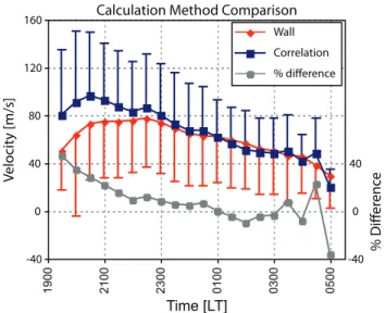
Fig. 2. Comparison of zonal drift velocity averages calculated by a
correlation routine and by an EPB west wall tracking routine as well as corresponding standard deviations. Note that the deviations are symmetric about the mean and, as such, they have only been plotted in one direction for each data set. The percent difference between the two results is also shown. This plot represents the averages of our entire data set.
data points, with one located around 22:00 LT and another around 00:30 LT. Figure 1b shows that our June solstice data contributes strongly to the second peak; this may reflect dis-creet seeding locations for EPBs in the Pacific sector (Makela et al., 2004) with seasonal variations, but more observations will be needed to verify this hypothesis and it is not addressed further in this paper.
3 Observations
In this section we detail the differences between the two cal-culation methods and analyze our data in terms of several influencing factors. All velocity figures present binned and averaged data that have also been run through a 3-point mov-ing average; standard deviation values for each time bin are also included on velocity figures using half-bars. We con-sider three variables as influencing factors: season, geomag-netic activity, and solar activity. Because an increase in ge-omagnetic activity may take many hours to influence drift velocities (Fejer et al., 2005), we have used Kp indices
av-eraged over 24-h periods in determining periods of high ge-omagnetic activity. We have defined days with averaged Kp
indices greater than or equal to 3 to be geomagnetically “dis-turbed” days, and we have labeled solar activity as “high” or “low” based on days with F10.7 indices greater than or
equal to 140 or less than 140, respectively. In making sea-sonal comparisons, our velocity points from the two equinox periods have been combined to obtain a larger data set. Sev-eral other studies have used this procedure as well, as drift
704 D. Yao and J. J. Makela: Analysis of equatorial plasma bubble zonal drift velocities
Calculation Method Comparison by Season Equinox 160 -40 0 40 80 120 V elocit y [m/s] Time [LT] 1900 2100 2300 0100 0300 0500 160 -40 0 40 80 120 V elocit y [m/s] Solstice Time [LT] 1900 2100 2300 0100 0300 0500 Correlation Wall
Fig. 3. Comparison of velocity calculation routines on quiet time data, divided by season, with equinox averages on the left and June solstice
averages on the right. A maximum difference of around 40% is observed during the equinox, compared with a maximum difference of around 20% during the June solstice period.
velocity behaves similarly in these seasons (Fejer et al., 2005; Liu et al., 2006). The December solstice period will not be discussed as the data from this period are sparse due to me-teorological conditions, contamination, and a general lack of EPBs during this season in the Pacific sector (Makela et al., 2004; Gentile et al., 2006). Thus, all plots labeled “solstice” denote the June solstice.
3.1 Velocity calculation method comparison
The averaged quiet time results of the entire observational period using both velocity-determining methods are shown in Fig. 2. Also shown in this figure is the percent difference between the two velocity-determining methods; ignoring the first and last points, which are less statistically significant, the correlation method gives results that are approximately 10–35% higher before 23:00 LT and within ±10% of the wall tracking routine after this time. This follows expecta-tions very well, as internal turbulence and bubble develop-ment take place earlier in the evening. Post-midnight, the majority of the depletions are “fossilized” in place and do not change in their east-west dimensions. As stated earlier, the correlation method, which makes use of information about the entire width of a given EPB, is sensitive to this type of development. Thus, we would expect our two independent methods to produce similar results only after a given EPB has fully developed.
This effect is not reflected equally in different time periods of our data. The difference is very pronounced in 2002 while later years show more comparable magnitudes at all local times (not shown here). The reasons for this are not entirely clear. However, it has been noted that depletions tend to form bifurcations and secondary instabilities more often closer to periods of solar maximum (Pimenta et al., 2001). Because the data from 2002 are closest to solar maximum it is possi-ble that the larger differences seen between the two
velocity-determining methods during this year are due to more active EPB development associated with high solar activity.
There are also seasonal differences between the velocity calculation methods, shown in Fig. 3. The correlation rou-tine returns velocities much higher than the wall tracking routine in equinox periods (up to 35% higher, not includ-ing end points), while solstice velocities are more compara-ble, showing the largest difference of 20% around local mid-night. It has been shown that the bifurcation and secondary instability growth dependence on solar activity is greatest in the equinox period (Pimenta et al., 2001), and extending this information to our data further corroborates the hypothesis stated above: the correlation method produces velocity re-sults contaminated by internal EPB dynamics.
3.2 Seasonal variations
As demonstrated above and pointed out by Pimenta et al. (2001), calculating velocities by tracking EPB west walls reduces bubble development effects and should thus be more representative of the background plasma drift velocity. In ad-dition, using this method will also allow us to better compare our results to previous studies which used a wall-tracking (or similar) method. Therefore, for the remainder of this study we will only present results from the wall tracking rou-tine. These results, separated by season, solar activity, and geomagnetic index, are presented in Fig. 4. In this figure, equinox averages are placed on the left side and June solstice averages are placed on the right side. The top row shows high solar flux conditions (F10.7≥140) while low solar flux
condi-tions (F10.7<140) are presented on the bottom. The amount
of data available per time bin for every case roughly matches the pattern of the corresponding seasonal totals displayed in Fig. 1 and does not have a significant effect on the corre-sponding average standard deviation magnitude.
160 -40 0 40 80 120 V elocit y [m/s] Time [LT] 1900 2100 2300 0100 0300 0500 160 -40 0 40 80 120 V elocit y [m/s] Time [LT] 1900 2100 2300 0100 0300 0500 160 -40 0 40 80 120 V elocit y [m/s] Time [LT] 1900 2100 2300 0100 0300 0500 160 -40 0 40 80 120 V elocit y [m/s] Time [LT] 1900 2100 2300 0100 0300 0500 Equinox Solstice High Flux Low Flux
Zonal Drift Velocities by Season, Solar Flux, and Geomagnetic Index
Kp < 3
Kp ≥ 3
Fig. 4. Zonal drift velocities divided by season, solar flux, and geomagnetic index. In this figure the combined equinox averages are presented
on the left side and the June solstice averages are presented on the right side. The upper two graphs represent averages for which the F10.7
index was greater than or equal to 140, while the lower two graphs represent averages for which the F10.7index was less than 140. Velocities
during geomagnetically disturbed conditions are plotted using blue lines and quiet time averages are plotted using red lines.
Concentrating first on the quiet time (Kp<3) high solar
flux numbers, we see a marked contrast between equinox and solstice conditions. During equinox, the maximum zonal eastward drift velocity of 100 m/s is reached at 22:30 LT be-fore decreasing to 60 m/s at 02:30 LT. A slight increase is seen at this time before the magnitudes continue to decrease until local sunrise. The velocities determined for the June solstice, on the other hand, peak at a zonal eastward velocity of less than 80 m/s at 22:30 LT before decreasing over the re-mainder of the night. Thus, during high solar flux conditions, we see an approximately 20% reduction in the mean zonal drift velocities from equinox to June solstice conditions.
In contrast to the high-flux results, the velocities are comparable in the different seasons during low-flux con-ditions. In both the equinox and the solstice periods, the eastward drift velocities remain approximately 80 m/s from 20:00–23:30 LT. After this time, the two seasonal drifts di-verge, with the average equinox drift decreasing to 40 m/s at 03:30 LT. The solstice drifts remain at 80 m/s until 01:00 LT before decreasing to 50 m/s at 03:30 LT.
There is also a significant seasonal difference between the geomagnetically disturbed drifts for both high and low solar flux cases. This difference is shown for the low-flux case in Fig. 5. Although the curves are comparable before 23:00 LT, the velocities after this time decrease for the equinox case,
160 -40 0 40 80 120 V elocit y [m/s] Time [LT] 1900 2100 2300 0100 0300 0500 Solstice Equinox
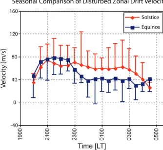
Seasonal Comparison of Disturbed Zonal Drift Velocities
Fig. 5. Comparison of drift velocities during geomagnetically
dis-turbed low solar flux conditions.
while they remain approximately constant for the solstice data until 03:00 LT. This suggests that larger storm-time ef-fects are present at equinox than solstice during low solar
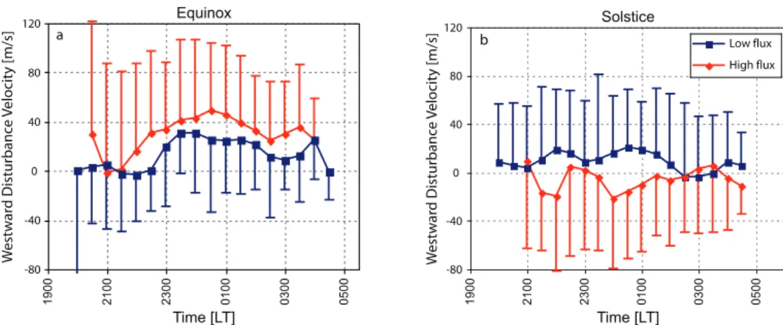
706 D. Yao and J. J. Makela: Analysis of equatorial plasma bubble zonal drift velocities 120 -80 -40 0 40 80 W estwar d Disturbanc e V elocit y [m/s] Time [LT] 1900 2100 2300 0100 0300 0500 120 -80 -40 0 40 80 W e stwar d Disturbanc e V elocit y [m/s] Time [LT] 1900 2100 2300 0100 0300 0500 Equinox Solstice
Perturbation Drift Velocities
Low flux High flux
a b
Fig. 6. Westward perturbation drift velocities, calculated by subtracting zonal drifts during geomagnetically disturbed conditions from quiet
time drifts, organized by solar flux level and season. In this figure positive numbers denote westward drifts.
flux conditions. A similar conclusion can be drawn from the high-flux disturbed data. During equinox, the average zonal drift velocity decreases from quiet-time averages, which is not the case for the solstice data. We discuss this further in Sect. 3.4.
3.3 Solar flux influences
Comparing the quiet-time equinox data at the different solar flux levels shown in Fig. 4 reveals lower zonal drift magni-tudes during low solar flux periods. After local midnight, however, the two become more comparable. Meanwhile, the June solstice velocity averages for low-Kpconditions show
the opposite trend, with decreased averages in high solar ac-tivity conditions compared to the low-flux case. However, when looking at peak velocities of individual nights, the June solstice data reflect very little dependence on solar activity. In fact, while a correlation analysis of the F10.7 index and
peak velocities on a nightly basis (not shown) returns a co-efficient of 0.40 during the equinox period, reflecting a mod-erate relationship between drift magnitudes and solar flux, this coefficient is −0.08 in the June solstice period, reflecting almost no immediate relationship between drift magnitudes and solar flux levels.
This seasonal difference in solar activity influence has been noted by Fejer et al. (2005). Interestingly, the correla-tion between solar flux levels and velocities is at least slightly higher for both seasons using the velocity results of our cor-relation analysis as opposed to our wall tracking routine (0.6 for the equinox data and 0.1 for the June solstice data). This is possibly another indication of increased EPB development during high levels of solar activity as discussed in Sect. 3.1.
It should be noted that the quiet time, high solar flux zonal velocity for both equinox and solstice conditions demon-strate greater variability than during low solar flux periods in terms of the standard deviation about the mean.
Averag-ing the four bins between 23:00 LT and 01:00 LT, a standard deviation of 47.2 m/s is estimated for the solstice season and a deviation of 48.9 m/s is measured for the equinox season during high-flux, low-Kp periods. As a comparison, during
low-flux, low-Kpperiods the average standard deviations
be-tween 23:00 and 01:00 LT are 39.8 and 37.7 for solstice and equinox conditions, respectively. This suggests that there is larger variability in the zonal velocity at high solar flux, even during non-storm conditions.
3.4 Geomagnetic influences
Significant differences are observed in our data between ge-omagnetically disturbed (Kp≥3) and quiet time (Kp<3)
ve-locities, especially during equinox conditions. These large equinox differences occur for periods of both high and low solar activity. To study this, we have calculated westward perturbation drifts during disturbed geomagnetic conditions by subtracting averaged velocities of disturbed nights from averaged quiet-time velocities of the same flux bins for the equinox season, a procedure also used by Fejer et al. (2005). The results are presented in Fig. 6a, in which the westward perturbation drifts are shown for nights of both high and low solar activity (in this figure positive denotes westward) dur-ing equinox. It can be seen in this figure that the perturba-tion drifts in the equinox season during low solar activity are only present in very low levels until 22:30 LT, after which the westward perturbation drifts increase very rapidly. This is even more apparent for periods of high solar flux, when a disturbance drift develops at 21:30 LT with a value of ap-proximately 50 m/s observed shortly after local midnight.
The effects of geomagnetic activity during solstice are not as straightforward, as shown in Fig. 6b. Similar to the re-sults for equinox, the low-flux solstice disturbance drifts ex-hibit westward perturbations between approximately 21:30 and 02:00 LT, but only at moderate levels (∼20 m/s). In
contrast to these results showing that an increase in geo-magnetic activity produces a westward perturbation oppos-ing the background velocity, the high-flux solstice data ac-tually shows an eastward perturbation velocity for much of the time period, enhancing the background velocity. This exemplifies the complex interactions between solar flux, ge-omagnetic activity, and season in determining the zonal drift velocities. Such variability in the relationship of the zonal velocity and geomagnetic activity has also been reported by Fejer et al. (2005) for zonal drift velocities over Jicamarca, Peru and by Liu et al. (2006) for the zonal thermospheric winds. Much work remains and more data need to be col-lected to understand these complex interactions.
4 Discussion
In general, the results presented here agree with velocity de-pendencies on solar and geomagnetic activity as well as over-all seasonal and temporal trends published in previous stud-ies. Although we are not able to examine the influence of high solar activity in more detail (especially in the June sol-stice period) due to comparatively less data from high solar flux conditions and large variations in the velocities calcu-lated from this data, it is clear that there exists a general dependence of the zonal drift velocity on solar flux in the Pacific sector for the equinox season, with higher velocities corresponding to higher solar flux levels. This correlation has been reported on extensively from measurements in other lo-cations (Martinis et al., 2003; Pimenta et al., 2003a; Immel et al., 2004; Fejer et al., 2005). The time variation of our data also matches these studies, with drift velocity dependency on flux levels decreasing after the early evening. From our data (Fig. 4) we see that high and low-flux equinox velocities be-come more comparable after 24:00 LT.
The most significant difference between our data and past studies is the lower magnitudes of our calculated drifts. Us-ing incoherent scatter radar data collected at the Jicamarca Radio Observatory, Fejer et al. (2005) generated a climato-logical model exhibiting zonal drift velocities that peak at 170 m/s (100 m/s) during equinox high (low) solar flux lev-els and 120 m/s (100 m/s) during solstice conditions. Also in the American sector, using optical techniques similar to those used in this study, peak eastward velocities on the order of 120–140 m/s are typically quoted (de Paula et al., 2002; Mar-tinis et al., 2003; Pimenta et al., 2003a, b). Several of these studies have observed a strong latitudinal variation (Marti-nis et al., 2002; Pimenta et al., 2003a). In the Indian sector, again using optical techniques, Mukherjee (2003) has pre-sented data from solar maximum equinox conditions with peak eastward velocities of over 175 m/s.
In addition to the drift data described above, Liu et al. (2006) have recently presented a climatology for equa-torial zonal winds obtained by accelerometer measurements from the CHAMP satellite. According to theoretical
consid-erations (Risbeth, 1971), the zonal neutral wind and plasma drift velocity are expected to be tightly coupled near the F-region peak at night. Many of the trends reported in the cur-rent study are also seen in the neutral wind climatology pre-sented by Liu et al. However, similar to the discrepancies pointed out above, the magnitudes of the velocities we have calculated are lower than those found in Liu et al.
There are several possible reasons for the discrepancy in drift velocity magnitudes between our data and those pre-sented in previous studies. First, we have assumed an emis-sion height of 250 km for the 630.0-nm airglow images. This may cause differences with velocities calculated using other instruments such as satellite in-situ measurements or scintil-lation data which measure velocities at different heights than the airglow technique. It has been shown that using an as-sumed emission height of 300 km results in velocities up to 20% higher (Pimenta, 2003b). Second, as is apparent from the discussion in Sect. 3.1, the method used to calculate drift velocities can have a large effect on the results. Third, be-cause velocities have a latitudinal (apex height) dependence, the geomagnetic latitudes of other studies must be consid-ered before making a direct comparison. Thus, one reason why the velocities calculated here are lower than those pre-sented in past studies could be the further poleward location of our instrument in relation to most other imager sites.
However, when compared with results which have been taken from approximately the same magnetic latitudinal sec-tor as Haleakala (such as the imager stations at Tucum´an, Argentina, and Cachoeira Paulista, Brazil), our observed ve-locities are still lower. At these South American stations, drift velocities have been reported to reach peaks of between 120 m/s and 140 m/s respectively (Martinis et al., 2003; Pi-menta et al., 2003a) from calculations using 630.0-nm data and the same assumed emission height as we have used here. The peak of 120 m/s reported in Martinis et al. (2003) was calculated during equinox periods of low solar activity, and this represents at 50% increase over our results under similar conditions. Differing calculation methods most likely cannot account for the discrepancy, as the maximum difference be-tween our correlation and wall tracking routines for the quiet time equinox period was 35%. The peak of 140 m/s reported in Pimenta et al. (2003a) was taken from data closer to solar maximum during the December solstice. This also represents a 50% increase from our results. Thus, while it is possible that our lower drift velocity results can be attributed to a va-riety of factors, we feel that the most likely explanation is a longitudinal dependence of zonal drift velocities.
Such a longitudinal variation of the zonal plasma drift was pointed out by Immel et al. (2004). Using data ob-tained by the IMAGE satellite, they showed a global zonal velocity peak in the Indian sector. This is corroborated by the Mukherjee (2003) results obtained using a ground-based imager, although the data presented only covered several months. Fejer et al. (2005) conjectured that a longitudinal dependence in zonal drift velocities should be expected due,
708 D. Yao and J. J. Makela: Analysis of equatorial plasma bubble zonal drift velocities in part, to the relationship between zonal and vertical drift
velocities, because the latter is known to have a longitudinal dependence (Scherliess and Fejer, 1999). We conclude, then, that the reduced zonal drift velocity magnitudes calculated from our Pacific sector data are direct observational evidence of this longitudinal dependence.
5 Summary
We have studied the seasonal, solar, and geomagnetic de-pendence of nighttime equatorial plasma drifts by calculat-ing EPB drift velocities. These data were obtained by an-alyzing nightglow images from a narrow-field imaging sys-tem located in the Pacific sector. Depletion velocities have been calculated using two different methods; the first method we have employed is a correlation calculation and the sec-ond is a west wall tracking routine suggested by Pimenta et al. (2001). Differences between these velocity calculation routines suggest pre-midnight EPB development and expan-sion of east-west dimenexpan-sions by bifurcations and secondary instabilities.
Our results for the most part are in good agreement with seasonal, solar, and geomagnetic trends reported in past stud-ies with the exception of overall lower magnitudes in drift velocities. Though there are a variety of possible reasons as to why our calculated velocities are lower than presented in other studies, the most probable is that the discrepancy is due to a longitudinal variation of zonal drift velocities. We plan to continue collecting data from CNFI to further corroborate our observations presented here, as well as to examine solar activity influences in more depth.
Acknowledgements. Work at the University of Illinois at
Urbana-Champaign was supported by NRL grant N00173-05-1-G904. The imager used in this study is supported by AFOSR grant F49620-01-1-0064 to Cornell University. We thank the staff at the Maui Space Surveillance Site for their continued support in operating the imaging system and M. C. Kelley for supporting the collection of the data used in this study.
Topical Editor M. Pinnock thanks two referees for their help in evaluating this paper.
References
Booker, H. G. and Wells, H. W.: Scattering of radio waves by the F-region of the ionosphere, Terr. Magn. Atmos. Elect., 43, 249– 256, 1938.
de Paula, E. R., Kantor, I. J., Sobral, J. H. A., Takahashi, H., Santana, D. C., Gobbi, D., de Medeiros, A. F., Limiro, L. A. T., Kil, H., Kintner, P. M., and Taylor, M. J.: Ionospheric ir-regularity zonal velocities over Cachoeira Paulista, J. Atmos. Solar-Terr. Phys., 64(12–14), 1511–1516, doi:10.10.16/S1364-6826(02)00088-3, 2002.
Fagundes, P. R., Sahai, Y., Batista, I. S., Bittencourt, J. A., and Taka-hashi, H.: Vertical and zonal equatorial F-region plasma bubble
velocities determined from OI 630 nm nightglow imaging, Adv. Space Res., 20, 1297–1300, 1997.
Fejer, B. G., de Souza, J., Santos, A. S., and Costa Pereira, A. E.: Climatology of F region zonal plasma drifts over Jicamarca, J. Geophys. Res., 110, A12310, doi:10.1029/2005JA011324, 2005. Garcia, F. J., Taylor, M. J., and Kelley, M. C.: Two-dimensional spectral analysis of mesospheric airglow image data, Appl. Opt., 26(29), 7374–7385, 1997.
Gentile, L. C., Burke, W. J., and Rich, F. J.: A climatology of equa-torial plasma bubbles from DMSP 1989–2004, Radio Sci., 41, RS5S21, doi:10.1029/2005RS003340, 2006.
Immel, T. J., Frey, H. U., Mende, S. B., and Sagawa, E.: Global observations of the zonal drift speed of equatorial ionospheric plasma bubbles, Ann. Geophys., 22, 3099–3107, 2004,
http://www.ann-geophys.net/22/3099/2004/.
Kelley, M. C.: The Earth’s Ionosphere, Academic, San Diego, Cal-ifornia, 1989.
Kelley, M. C., Makela, J. J., Ledvina, B. M., and Kintner, P. M.: Ob-servations of equatorial spread-F from Haleakala, Hawaii, Geo-phys. Res. Lett., 29(20), doi:10.1029/2002GL015509, 2002. Kintner, P. M., Ledvina, B. M., de Paula, E. R., and
Kan-tor, I. J.: Size, shape, orientation, speed, and duration of
GPS equatorial anomaly scintillations, Radio Sci., 39, RS2012, doi:10.1029/2003RS002878, 2004.
Link, R. and Cogger, L. L.: A reexamination of the OI 6300 ˚A
nightglow, J. Geophys. Res., 93(A9), 9883–9892, 1988. Liu, H., L¨uhr, H., Watanabe, S., K¨ohler, W., Henize, V.,
and Visser, P.: Zonal winds in the equatorial upper
ther-mosphere: Decomposing the solar flux, geomagnetic activity, and seasonal dependencies, J. Geophys. Res., 111, A07307, doi:10.1029/2005JA011415, 2006.
Makela, J. J. and Kelley, M. C.: Field-aligned 777.4-nm composite airglow images of equatorial plasma depletions, Geophys. Res. Lett., 30(8), 1442, doi:10.1029/2003GL017106, 2003.
Makela, J. J., Ledvina, B. M., Kelley, M. C., and Kintner, P. M.: Analysis of the seasonal variations of equatorial plasma bubble occurrence observed from Haleakala, Hawaii, Ann. Geophys., 22, 3109–3121, 2004,
http://www.ann-geophys.net/22/3109/2004/.
Makela, J. J., Kelley, M. C., and Su, S.-Y.:
Simultane-ous observations of convective ionospheric storms: ROCSAT-1 and ground-based imagers, Space Weather, 3, SROCSAT-12C02, doi:10.1029/2005SW000164, 2005.
Martinis, C., Eccles, J. V., Baumgardner, J., Manzano, J., and Mendillo, M.: Latitude dependence of zonal plasma drifts ob-tained from dual-site airglow observations, J. Geophys. Res., 108(A3), 1129, doi:10.1029/2002JA009462, 2003.
Mendillo, M. and Baumgardner, J.: Airglow characteristics of equa-torial plasma depletions, J. Geophys. Res., 87, 7641–7652, 1982. Mukherjee, G. K.: Studies of the equatorial F-region depletions and dynamics using multiple wavelength nightglow imaging, J. At-mos. Solar-Terr. Phys., 65(3), 379–390, 2003.
Pimenta, A. A., Fagundes, P. R., Bittencourt, J. A., Sahai, Y., Gobbi, D., Medeiros, A. F., Taylor, M. J., and Takahashi, H.: Ionospheric plasma bubble zonal drift: a methodology using OI 630 nm all-sky imaging systems, Adv. Space Res., 27, 1219– 1224, 2001.
Pimenta, A. A., Fagundes, P. R., Bittencourt, J. A., Sahai, Y., Buriti, R. A., Takahashi, H., and Taylor, M. J.: Ionospheric plasma
ble zonal drifts over the tropical region: a study using OI 630 nm emission all-sky images, J. Atmos. Solar-Terr. Phys., 65, 1117– 1126, 2003a.
Pimenta, A. A., Fagundes, P. R., Sahai, Y., Bittencourt, J. A., and Abalde, J. R.: Equatorial F-region plasma depletion drifts: lati-tudinal and seasonal variations, Ann. Geophys, 21, 2315–2322, 2003b.
Rishbeth, H.: Polarization fields produced by winds in the equato-rial F-region, Planet. Space Sci., 19, 357–369, 1971.
Scherliess, L. and Fejer, B. G.: Radar and satellite global equatorial F region vertical drift model, J. Geophys. Res., 104, 6829–6842, 1999.
Su, S.-Y., Yeh, H. C., and Heelis, R. A.: ROCSAT 1 ionosphric plasma and electrodynamics instrument observations of equato-rial spread F: An early transitional scale result (2001), J. Geo-phys. Res., 106(A12), 29 153–29 159, 2001.
Taylor, M. J., Eccles, J. V., LaBelle, J., and Sobral, J. A. H.: High resolution OI 630 nm image measurement of F-region depletion drifts during the Guara campaign, Geophys. Res. Lett., 24, 1699– 1702, 1997.
Tinsley, B. A.: Field aligned airglow observations of transequatorial bubbles in the tropical F-region, J. Atmos. Terr. Phys., 44(6), 547–557, 1982.
Tinsley, B. A., Rohrbaugh, R. P., and Hanson, W. B.: Images of transequatorial F region bubbles in 630- and 777.4-nm emissions compared with satellite measurements, J. Geophys. Res., 102, 2057–2077, 1997.
Valladares, C. E., Meriwether, J. W., Sheehan, R., and Biondi, M. A.: Correlative study of neutral winds and scintillation drifts measured near the magnetic equator, J. Geophys. Res., 107(A7), 1112, doi:10.1029:2001JA000042, 2002.