Multifractal modelling and simulation of rain fields exhibiting spatial heterogeneity

HAL Id: hal-00304720

https://hal.archives-ouvertes.fr/hal-00304720

Submitted on 1 Jan 2002

HAL is a multi-disciplinary open access

archive for the deposit and dissemination of sci-entific research documents, whether they are pub-lished or not. The documents may come from teaching and research institutions in France or abroad, or from public or private research centers.

L’archive ouverte pluridisciplinaire HAL, est destinée au dépôt et à la diffusion de documents scientifiques de niveau recherche, publiés ou non, émanant des établissements d’enseignement et de recherche français ou étrangers, des laboratoires publics ou privés.

exhibiting spatial heterogeneity

A. Pathirana, S. Herath

To cite this version:

A. Pathirana, S. Herath. Multifractal modelling and simulation of rain fields exhibiting spatial het-erogeneity. Hydrology and Earth System Sciences Discussions, European Geosciences Union, 2002, 6 (4), pp.695-708. �hal-00304720�

Multifractal modelling and simulation of rain fields exhibiting

spatial heterogeneity

Assela Pathirana

1

_{and Srikantha Herath}

2

1_{Faculty of Science and Engineering, Chuo University, Kasuga, Bunkyo-ku, Tokyo, Japan} 2_{Institute of Industrial Science, University of Tokyo, Komaba, Meguro, Tokyo, Japan}

Email for corresponding author: [email protected]

Abstract

Spatial multifractals are statistically homogeneous random fields. While being useful to model geophysical fields exhibiting a high degree of variability and discontinuity and including rainfall, they ignore the spatial trends embedded in the variability that are evident from large temporal aggregation of spatial fields. The modelling of rain fields using multifractals causes the information related to spatial heterogeneity, immensely important at some spatial scales, to be lost in the modelling process. A simple method to avoid this loss of the heterogeneity information is proposed. Instead of modelling rain fields directly as multifractals, a derived field M is modelled; this is the product of filtering observed rainfall snapshots with spatial heterogeneity as indicated by long term accumulations of rain fields. The validity of considering the field M as multifractal is investigated empirically. The applicability of the proposed method is demonstrated using a discrete cascade model on gauge-calibrated radar rainfall of central Japan at a daily scale. Important parameters of spatial rainfall, like the distribution of wet areas, spatial autocorrelation and rainfall intensity distributions at different geographic locations with different amounts of average rainfall, were faithfully reproduced by the proposed method.

Keywords: spatial rainfall, downscaling, multifractals

Introduction

Investigations of weather and climatic systems at a global scale have become a prime area of research for a number of reasons among which the concern about global climatic change is a main one. In addition to an increased scientific understanding of atmospheric processes, many useful forecasting products have become available. These include regional and global climatic models, which predict short-term weather patterns and longer short-term trends in climate at a coarser scale. Hydrologists are often involved in solving problems that concern much smaller scales than those of global or regional models. Many attempts have been made in the past to bridge the gap between the regional and the catchment scale.

Deterministic resolving of spatial rainfall at sub-grid scale cannot be achieved with only the information provided by large-scale forcing. The simplest scheme to distribute rainfall at sub-grid scale would be to distribute it uniformly. In spite of being unrealistic, this can work in preserving the overall conservation of water, if the ‘receiving medium’ (i.e.

physical governing equations related to surface hydrology) for a particular problem is approximately linear. However, for most of the problems related to the operational use of spatial rainfall at catchment level, this is hardly the case. Examples are operational flood risk analysis, urban drainage problems that involve evaluation of infiltration and long-term water resources studies requiring reliable estimation of evaporation. A better approach is to distribute rainfall using a predetermined distribution (like the exponential distribution explained by Shuttleworth (1988) acknowledging the work of others,) which can be used to reduce errors resulting from the nonlinearity of the governing equations, like those for evaporation and infiltration, by distributing rainfall in a nonlinear fashion. Another approach, that has recently become popular, is to use multifractal theory to downscale rainfall to sub-grid levels. Rainfall is assumed to be a multifractal process characterised by spatial discontinuities and spatial variability. By adopting this model, rainfall variability in

Numerous random cascade based models to represent the variability of rainfall have been reported in the literature. Some of them involve assumptions of certain mathematical model behaviour justified by empirical evidence and physically-based reasoning (Lovejoy and Mandelbrot, 1985; Tessier et al., 1993; Gupta and Waymire, 1990b) while others used the cascade process empirically (Olsson, 1998; Lammering and Dwyer, 2000).

Spatial rainfall maps of small temporal integration sizes such as hourly or daily scales seem to be random. As multiplicative cascades are themselves random models, they can explain such spatial distributions quite well. However, when, by averaging a large number of spatial snapshots, the time integration is increased to a monthly or seasonal scale, the observed spatial rainfall becomes less random and, in most cases, more heterogeneous. This indicates that even at small temporal aggregations, spatial fields have the spatial heterogeneity embedded in the variability but this is masked by (stronger) random variability. Numerous features of regional rainfall, including orographic enhancement and slope aspect - wind direction interactions, can be responsible for this observation. Figure 2 shows the average spatial rainfall for January, May and July for the central part of Japan. In January, the rainfall amount is relatively large on the northwestern slopes due to northern winds in winter, while summer causes high rainfall in the Kii peninsula (at the bottom left of the map).

Multifractal models used to describe spatial rainfall are spatially homogeneous in a statistical sense. This means that large accumulations of such snapshots result in spatially homogeneous fields. Though this type of modelling ignores any systematic variability of the process at various sub-domains, it does not prevent the effective use of multifractal models as diagnostic tools. For example, Olsson and Niemczynowicz (1996) analysed daily spatial rainfall of southern Sweden to show that rainfall arising from different meteorological processes results in distinctly different scaling properties. In fact this ‘lumping’ of properties is, by definition, a feature in any type of statistical study. However, the application of not only multifractal models, but also any type of statistical model, requires the assurance that the model does transfer all the properties of observed data that are significant for the particular purpose at hand. From this operational point of view, a drawback of using just multifractals to model spatial rainfall is that the information regarding the spatial heterogeneity that is an important feature of observed rainfall will be lost during the modelling process. Any approach based only on (‘lumped’) multifractal characteristics would fail to maintain the spatial heterogeneity inherently present in rainfall patterns over many geographical areas.

0 50 100 0 50 100 0 50 100 0 50 100

Step 0

Step 3

Step 2

Step 1

Ro

R1,1

R1,2

R1,3

R1,4

L

L

L/2

L/2

L/4

L/4

L/8

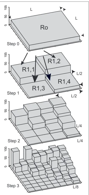
Fig. 1. A multiplicative cascade process in two dimensions. Here

each box is subdivided into four boxes at each stage. This

subdivision number is called the branching number, b. For any value of b (e.g. 4, 9, 16, 25, . . . ), the scale ratio λnat the cascade step n,

can be expressed as: λn=bn/d where d is the embedding dimension

In operational problems like flood risk analysis, the accurate representation of spatial heterogeneity is as important as the precise modelling of spatial variability. For example, if an upstream mountainous area in a catchment receives significantly more rainfall than a low-lying area downstream, flood magnitude and duration estimates for such a catchment can be substantially distorted by treating spatial variability without considering spatial heterogeneity explicitly.

Jothityangkoon et al. (2000) incorporated spatial heterogeneity in multifractal simulation and evaluated the performance of the model using spatial rainfall data from Australia. The explicit random cascade process used to distribute rainfall at sub-grid level, incorporated the spatial heterogeneity. In the present paper, a simpler method is used to incorporate spatial heterogeneity in downscaled spatial rainfall and the outcome is compared with that of the Jothityangkoon et al. (2000) method.

The proposed modification can be used irrespective of the specific multifractal theory used to model the random variability of spatial rainfall. While numerous suitable models are available (Tessier et al., 1993; Meneveau and Sreenivasan, 1987; Gupta and Waymire, 1990b; Deidda et

al., 1999; Menabde et al. 1999; Lammering and Dwyer,

2000), one with minimum complexity and wide application was selected to demonstrate the proposed modification.

PROPOSED MODEL

Rainfall is considered a combined effect of two processes, (1) a multifractal process which is highly variable in space but, at least at regional and smaller scales, statistically uniform over the area concerned, and (2) a process that represents the heterogeneity of rainfall in space that is used to ‘modify’ the above multifractal process. The most general

case is that both these components should be stochastic (random). However, for simplicity, it is assumed that the randomness of the rainfall is provided solely by the multifractal component and the heterogeneity is deterministic. At this stage, a rigorous physical interpretation of this separation is not attempted, though it is possible to visualize it in the following way: The cloud positioning in a flat area small enough to ignore global circulation patterns, can be assumed to be random. However, when clouds move over a land area with significant topographical features, the generation of rainfall is affected both by the position of the cloud and the topographical features such as mountains. This can be considered as a ‘modification’ of (random) cloud positioning by a deterministic process that represents the local topography. (However, this localised effect may not be caused only by the orography.) Hence, the rainfall over a small period of time seems to be random because it is a mixture of random and deterministic components. When the rainfall is accumulated over a long time period, the randomness reduces to a uniform field due to the averaging effect, and hence, the deterministic effect predominates. This can explain the marked heterogeneity observed in large accumulations. As the accumulation length is increased, the random effect becomes dormant and the heterogeneity becomes more obvious. However, in practice, this is true only if similar rainfalls (e.g. same season) are accumulated. For example, if the rainfall of Japan is accumulated over all the seasons, the winter and summer rainfalls may compensate each other to a large degree, and produce a more uniform field than the winter or summer rainfall taken separately. 136º 138º 140º 142º 34º 36º 38º 0 100 200 km 136º 138º 140º 142º 34º 36º 38º 136º 138º 140º 142º 34º 36º 38º 0 100 200 km 136º 138º 140º 142º 34º 36º 38º 136º 138º 140º 142º 34º 36º 38º 0 100 200 km 136º 138º 140º 142º 34º 36º 38º 0 5 10 15 20 25

Fig. 2. Spatial heterogeneity shown by the daily average rainfall intensities for the months of January (left) May (middle) and July (right),

Mathematical development

The following equation expresses the proposed model in mathematical notation: j i j i j i

M

G

R

_,

=

_{, ,} ,    = = _{R G}forG_otherwise M j i j i j i j i , , , , _/ 0 0 (1)

where R_i,j is the rainfall on the pixel (i,j) and G_i,j is the

component of that rainfall that is invariant over a long accumulation. It is assumed that it can be represented adequately by the long-term seasonal average. Then, by

definition, M_i,j is a component that is randomly distributed

in the space so that M yields a uniform field at large accumulations. Hence M is a candidate for multifractal modelling.

To keep the model simple, the temporal progression of the rainfall is neglected. Thus, a key assumption of the present model is that the rainfall of a given snapshot is independent of the other snapshots. For small time steps like hourly rainfall, this may not be true, for the movement of rainfall over an area cannot be neglected at such a small temporal scale.

Rainfall data

The operational radar rainfall composites (referred to as Radar-AMeDAS hereafter) published by the Japan Meteorological Agency (JMA), generally cover the whole Japanese archipelago. JMA uses 19 conventional weather radars with 400 km radial coverage (except for the Mt. Fuji radar which covers 800km) to provide hourly rainfall estimates at an average of 8 scans per hour. These data, with a resolution of 2.5 km are converted to 5 km resolution and then calibrated with the extensive hourly rain gauge network, popularly known as AMeDAS, to correct for errors arising from the instability of the sensitivity of the radar hardware and due to the vertical variation of rainfall (Makihara, 1996). The final product is hourly-calibrated spatial rainfall data of land and surrounding sea with a grid

size of approximately 5km (0.06250 _{in longitude and 0.05}0

in latitude). An area of 128x128 pixels bounded by 39.65N 134.5W, 33.3S and 142.4375E was selected for the study. The rainfall precision is 1mm (with an additional value at 0.4mm).

As the model takes no account of the temporal correlation of rainfall events that occurs at small accumulation sizes, it was tested at a daily scale. Daily rainfall snapshots were created by summing the 24 hourly snapshots of the day. The spatial heterogeneity of rainfall varies with the season (Fig. 2). Hence, rainfall of different seasons must be

modelled separately, to capture the spatial heterogeneity correctly. In the present research, each month was modelled as a different season. Since the data for the period of 1995– 1999 were available for analysis, the number of snapshots available for model fitting for a given month was about 150.

Multifractal model

A multifractal model is needed to represent M (Eqn. 1). The β-lognormal model proposed by Over and Gupta (1996) was used because of its simplicity, wide application and the ability to treat zero rainfall areas explicitly.

Figure 1 shows an example of a multiplicative cascade

process. The branching number b is given by N_i+1/N_i= b

where N_iis the total number of segments at cascade step i.

At each cascade step, each segment is divided into b equal parts and each part is multiplied by a value (cascade weight) drawn from a specified distribution, which is known as the

generator of the cascade. One of the simplest cascade

models is the β-model, whose generator is specified by:

β −

−

=

=

b

W

P

(

0

)

1

, P(W =bβ)=b−β (2)

where W is the cascade weight and b is a model parameter. This model can represent the presence and absence of values in a distribution. When a lognormal distribution is used as generator the resulting cascade is known as a lognormal cascade. Over and Gupta (1996) combined the above two cascade models to propose a b-lognormal model given by:

β σ σ β− + ₋ = =b b W P X b ) ( 2 ] log[ 2 β − − = = b W P( 0) 1 (3)

where β and σ2 _{are model parameters. X is a standard normal}

variable. This is a conserved cascade scheme, for the formulation maintains the expected value of W,

1

)

(

w

=

E

PARAMETER EVALUATION FOR LOGNORMAL MODEL

A multiplicative cascade shows the following scaling behaviour:

∑

= = i q q i R q M ( ) , ] [ ) , ( τ λ λ λ (4)

where R_i,λ is the value of the field at the ith box at the scale

)

1

]

[

0

)

1

(

[ 2log( )/2

=

=

−

_b

−β

_E

_b

−σ b +σX [( ) ( 2log( )/2 + =_{E b}− _b− − b + X W E β β σ σ

λ (λ=L/l where l is scale and L is the largest scale of interest.) The order of statistical moment is q.

Over and Gupta (1994, 1996) proposed the concept of a Mandelbrot-Kahane-Peyriere (MKP) function to estimate

model parameters for the β-lognormal model. MKP

function, χ(q), of a multiplicative cascade process, is defined

as the slope of the statistical moment M(_{λ,q) (Eqn. 4) to the}

cascade step n (Fig. 1).

Given that the cascade follows the scaling law

M(λ,q)=λτ(q)_{, the MKP function for the cascade is (by}

definition of the MKP function) τ(q)/d. Over and Gupta

(1996) derived the following expression for the MKP

function for the β-lognormal model:

_χ(_q)₌(_β−1)(_q−1)₊(_σ2ln(_b)/2)/(_q2_−q) ₍₅₎

By considering the first and second derivatives of

χ

q with

respect to q, _σ2 _{and β can be derived as follows:}

) ln( ) ( ) 2 ( 2 b d q τ σ = ; 2 ) 1 2 )( ln( ) ( 1 2 ) 1 ( − + + = b q d q σ τ β (6)

where b is the branching number (Fig. 1), and d is the embedding dimension ( d=2, for spatial rainfall). The values

ofσ2 _{and β can be evaluated numerically by computing the}

value of derivatives of τ(q) at some value of q. It is customary

to use q=1 .

One of the main advantages of using the β-lognormal

model to represent rainfall is its ability to incorporate non-rainy pixels explicitly. This avoids the problems related to applying arbitrary cut-off intensities to introduce zero values to model generated fields. The use of the lognormal generator which has an analytical expression and the transparent cascade scheme makes this an easy model to implement. The use of lognormal cascades (which, mathematically is a special case of a broad class known as Lévy-stable distributions.) to model rain fields, has been questioned in the literature (e.g. Tessier et al., 1993). However, this issue is still undecided and is outside the scope of the present research.

Methodology for model construction

As expressed in Eqn.1, the most important step in model construction is to ‘filter’ the observed rain fields to obtain

M fields, which are spatially homogeneous in a statistical

sense. To compute the field G for a given month, all the snapshots for that month were averaged at pixel level as:

∑

= = ' 1 , , , _' 1 N k k j i j i _N R A (7)

∑

= ij _ij ij j i TA A G_{, ,} / _{, ,} (8)

where N’ is the number of snapshots with the value (i, j) present and T is the total number of pixels in a snapshot. In

other words, G_i,jis the field of normalized long-term averages

used to represent the spatial heterogeneity.

For each snapshot, R, a field of M is obtained by applying the relationship in Eqn.1. After obtaining the M fields, the next step was to test whether it is possible to model M as a multifractal model. Although rainfall distributions in two-dimensions have been verified as multifractal on numerous occasions in the past, this is essential since M is only a field derived from observed rainfall, newly introduced in the present work.

SCALING OF M

It is customary to normalise each snapshot to have unit mean before performing multifractal analysis. The statistical

moment M(λ, q) (Eqn. 4) is calculated for different values

of q and scale, λ. Since the data space for a single snapshot

is 128 × 128 pixels, the largest scale was selected as L = 128. The range of scales available for analysis was from

log₂λ = 7 (boxsize, l = 1pixel) to log2λ = 2 (l = 32). The

latter limit is due to the small number of ‘boxes’ to compute the moment at larger box sizes. Figure 3 shows sample results of these moment calculations. The power-law

behaviour of M(λ, q) (i.e. linearity of the plot of log[M(λ,

q] against the log [λ]) indicates that M field shows excellent scaling properties. This justifies the use of a cascade model to represent M. Using the above estimations, the scaling

exponent, τ(q) can be evaluated as the slope of log[M(λ,q)]

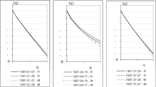
v. log[λ] curves for various values of q. The shape of the τ(q) curve is sensitive to the scaling properties of the rain field. For example, a linear curve indicates simple (as opposed to multiple) scaling properties. Figure 4 shows

some examples of τ(q) functions estimated from M as well

as R fields. All curves show some degree of curvature, while that for the month of April is the highest. Further, it shows that, in general, the scaling properties of R and M are not identical.

MODEL SETUP

Once the scaling properties of M are established, Eqn. 6 can be used to evaluate cascading model parameters. This essentially involves the estimation of the first and second

0 10 20 30 40 50 60 70 80 1 3 5 7 Log2[M(λ ,q)] Log2[λ] q=6.0 q=2.0 q=2.5 q=3.0 q=3.5 q=4.0 q=4.5 q=5.0 q=5.5 q=1.0 q=1.5 q=0.5 q=0.0 1997-Apr-03 M 0 10 20 30 40 50 60 70 80 1 3 5 7 Log₂[M(λ ,q)] Log₂[λ ] q=6.0 q=2.0 q=2.5 q=3.0 q=3.5 q=4.0 q=4.5 q=5.0 q=5.5 q=1.0 q=1.5 q=0.5 q=0.0 1997-Apr-03 R 0 10 20 30 40 50 60 70 80 1 3 5 7 Log₂[M(λ,q)] Log2[λ ] q=6.0 q=2.0 q=2.5 q=3.0 q=3.5 q=4.0 q=4.5 q=5.0 q=5.5 q=1.0 q=1.5 q=0.5 q=0.0 1997-Oct-30 R 0 10 20 30 40 50 60 70 80 1 3 5 7 Log₂[M(λ ,q)] Log2[λ] q=6.0 q=2.0 q=2.5 q=3.0 q=3.5 q=4.0 q=4.5 q=5.0 q=5.5 q=1.0 q=1.5 q=0.5 q=0.0 1997-Oct-30 M

Fig. 3. The scaling properties of statistical moment, M(λ, q) for rainfall snapshots of two selected dates. Moments are calculated

from both observed rainfall fields, R (left) and spatially homogeneous rainfall fields, M (right).

-6 -q (q) -6 -q (q) -6 -q (q)

Fig. 4. Estimations of _{τ(q) from R and M fields. Two examples each are shown for the months of January}

(left), April (middle) and July (right). The curvature of the function shows the degree of multiple scaling of the fields. Straight lines indicate simple scaling.

for this task. Firstly, a finite difference scheme was used to evaluate first and second derivatives around q=1. This

requires the estimation of values of τ(q) for three different

values around q=1. Secondly, a simple polynomial curve of order two or three was fitted to a number of estimations around q=1. The second method is less sensitive to local fluctuations due to small estimation errors. However, for the present problem both the techniques provided very close values.

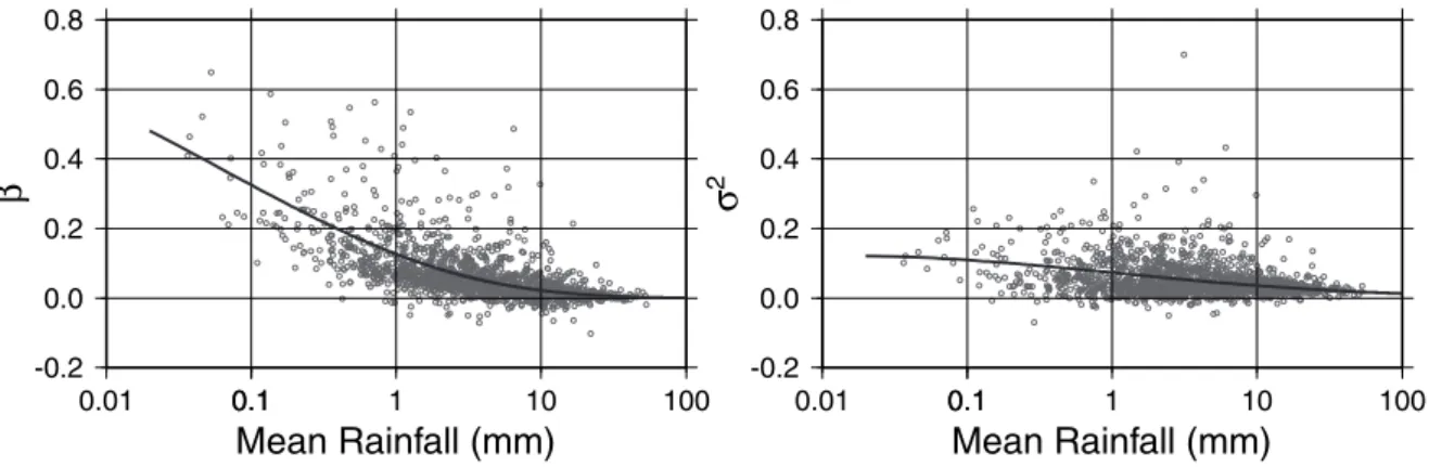
It is a well-established fact that rainfall distribution

properties are related to the average rainfall amount (also known as large-scale forcing). Values estimated for model

parameters β and σ2 _{were tested for dependency on large}

scale forcing (Fig. 5). The empirical functions ( _Rb

a = β and ] log ) (log exp[ 2 2 _{= k R +m R+n}

σ ) were used after

Jothityangkoon et al. (2000). The sensitivity of σ2 _{to the}

average rainfall is very much less than that of β, as reported previously by Over and Gupta, (1996). It was decided that

a constant value of (0.1) is adequate for simulation purposes.

It should be noted that the graphs in Fig. 5 are for the parameter values for all the months put together. Examination of individual months showed that employing a separate regression relationship (or a single value in the

case of σ2_{) for each month does not improve the}

relationships.

Simulation

Typical use of the proposed model is the distribution of a given rainfall amount at sub-grid scales, preserving the degree of spatial variability (randomness) and spatial heterogeneity as indicated by historical data. The first step in simulation of a rainfall field is the selection of cascade model parameters based on the average rainfall amount (or the large-scale forcing), for which the regression relationships established earlier can be used. Then, the

appropriate number of cascade steps are performed on a initial distribution of uniform unit intensity. To arrive at the

nth cascade step from the (n-1)th step (cascade step notation

according to Fig.1), 22n _{values for the cascade weight W are}

needed. To derive a value of W, firstly, the β-model is used to decide whether the particular value is zero or non-zero. Then, only for non-zero results, a value for W is drawn from the following distribution:

X b b W = β−σ 2 +σ ) log( 2 (9) where X is a standard normal variable.

The multifractal field M is obtained after seven cascade steps in the present case. This field is statistically homogeneous in space. The following equation (based on Eqn. 1) is used to modify M to obtain the synthetic distribution of rainfall R, which shows the spatial heterogeneity as observed rain fields:

∑

= j i j i j i j i j i j i AM G M G R , , , , , , / ( ) (10)

where A is the large-scale forcing.

Model validation

The objective of the model validation was to evaluate the proposed model’s ability to distribute a single amount of rainfall (large-scale forcing) into the constituent spatial grids. While it is possible to use a series of large-scale forcing values forecast by a regional scale atmospheric model for this purpose (which is one of the potential uses of the proposal), such an approach will incorporate in the validation process all the discrepancies between small-scale observations and the large-scale forecast. Thus, the spatially integrated values of the observed spatial rainfall fields were used as large-scale forcing values. To facilitate the most

-0.2 0.0 0.2 0.4 0.6 0.8 β 0.01 0.10.1 1 10 100 Mean Rainfall (mm) -0.2 0.0 0.2 0.4 0.6 0.8 σ 2 0.01 0.10.1 1 10 100 Mean Rainfall (mm)

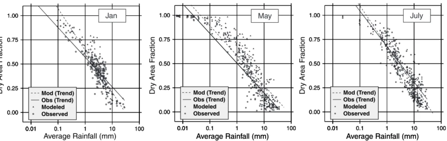
objective evaluation of the model’s working, each snapshot of the series of daily spatial rainfall maps used for the model setup (for years 1995–1999), was spatially integrated to provide a series of large scale forcing values for model input. A synthetic rainfall field was generated for each day by inputting in the model the corresponding value of large-scale forcing. The resulting set of about 1800 synthetic fields (about 150 for a single month) was compared, statistically, with the daily rainfall snapshots originally observed. Firstly, the fraction of dry areas was compared in modelled and observed distributions. For all the months, the distribution of dry fraction with average rainfall amount for modelled rainfall showed close agreement with observations. Figure 6 shows the dry-fraction of both synthetic and observed rain fields as functions of average rainfall amounts for the months of January, May and July. Figure 7 shows the average spatial rainfall for the months of January, May and July. Comparison of these with the

observed average rainfall fields in Fig. 2 shows that the spatial heterogeneity present in observed rainfall is reproduced in the modelled fields.

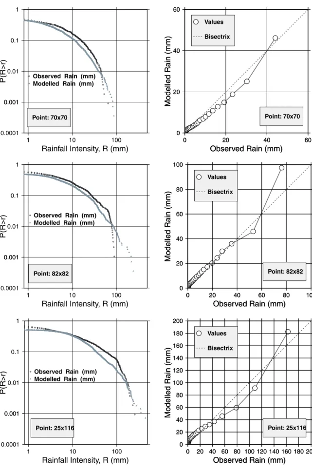
The following method was used to test quantitatively, the ability of the model to represent spatial heterogeneity. A number of locations for sampling rainfall was selected in the study area and around each point a 3 × 3 pixel window was sampled. Thus, for a single month, about 150 × 9 = 1350 values were available to estimate the exceedance probability curve of the rainfall intensity at the selected point. Figure 7 shows some selected points each for the months of January, May and July for the above analysis. The intensity distributions obtained for the months of May and July are shown in Figs. 8 and 9 respectively. It should be considered that the three points for each month comprise a point each from an area with highest, medium and lowest average rainfall for that month. These figures show that the intensity distributions at locations, whose

0.00 0.25 0.50 0.75 1.00 Dr y Area F raction 0.01 0.01 0.1 1 10 100 Average Rainfall (mm) 0.00 0.25 0.50 0.75 1.00 0.01 0.01 0.1 1 10 100 Average Rainfall (mm) Observed Modeled Obs (Trend) Mod (Trend) 0.00 0.25 0.50 0.75 1.00 Dr y Area F raction 0.01 0.01 0.1 1 10 100 Average Rainfall (mm) 0.00 0.25 0.50 0.75 1.00 0.01 0.01 0.1 1 10 100 Average Rainfall (mm) Observed Modeled Obs (Trend) Mod (Trend) May July 0.00 0.25 0.50 0.75 1.00 0.01 0.01 0.1 1 10 100 0.00 0.25 0.50 0.75 1.00 0.01 0.01 0.1 1 10 100 Observed Modeled Obs (Trend) Mod (Trend) Dr y Area F raction Average Rainfall (mm) Jan

Fig. 6. Dry fraction distribution of observed and simulated rainfall. Trend lines for an exponential relationship

(Dry Fraction

_∝

exp [Mean Rainfall]) are also shown.

136º 138º 140º 142º 34º 36º 38º 0 100 200

km

(60,68) (35,83) (020,120) 136º 138º 140º 142º 34º 36º 38º 136º 138º 140º 142º 34º 36º 38º 0 100 200

km

(70,70) (82,82) (25,116) 136º 138º 140º 142º 34º 36º 38º 136º 138º 140º 142º 34º 36º 38º 0 100 200

km

(85,82) (21,83) 136º 138º 140º 142º 34º 36º 38º 0 5 10 15 20 25

Fig. 7. Spatial heterogeneity shown by daily average rainfall snapshots for the months of January (left), May (middle) and July (right) for

simulated rainfall. Compare these maps with those in Fig. 2. The sample locations whose statistical distributions of the intensity ensembles are also shown.

0.0001 0.001 0.001 0.01 0.1 1 P(R>r) 1 1 10 100 Rainfall Intensity, R (mm) Observed Rain (mm) Modelled Rain (mm) Point: 82x82 0 20 40 60 80 100 Modelled Rain (mm) 0 20 40 60 80 100 Observed Rain (mm) 0 20 40 60 80 100 Modelled Rain (mm) 0 20 40 60 80 100 Observed Rain (mm) Values Point: 82x82 Bisectrix 0.0001 0.001 0.001 0.01 0.1 1 P(R>r) 1 1 10 100 Rainfall Intensity, R (mm) Observed Rain (mm) Modelled Rain (mm) 0 20 40 60 Modelled Rain (mm) 0 20 40 60 Observed Rain (mm) 0 20 40 60 Modelled Rain (mm) 0 20 40 60 Observed Rain (mm) Values Point: 70x70 Bisectrix 0.0001 0.001 0.001 0.01 0.1 1 P(R>r) 1 1 10 100 Rainfall Intensity, R (mm) Observed Rain (mm) Modelled Rain (mm) 0 20 40 60 80 100 120 140 160 180 200 Modelled Rain (mm) 0 20 40 60 80 100 120 140 160 180 200 Observed Rain (mm) 0 20 40 60 80 100 120 140 160 180 200 Modelled Rain (mm) 0 20 40 60 80 100 120 140 160 180 200 Observed Rain (mm) Values Point: 25x116 Bisectrix Point: 70x70 Point: 25x116

Fig. 8. Comparison of the rainfall intensities at sample points for May.(left): Exceedance probabilities. (right):

0 20 40 60 80

Modelled Rain (mm)

0 20 40 60 80 Observed Rain (mm) 0 20 40 60 80

Modelled Rain (mm)

0 20 40 60 80 Observed Rain (mm) Values Point: 60x68 Bisectrix 0 20 40 60 80 100 120 140 160

Modelled Rain (mm)

0 20 40 60 80 100 120 140 160 Observed Rain (mm) 0 20 40 60 80 100 120 140 160

Modelled Rain (mm)

0 20 40 60 80 100 120 140 160 Observed Rain (mm) Values Point: 35x83 Bisectrix 0 40 80 120 160 200 240 280 320

Modelled Rain (mm)

0 40 80 120 160 200 240 280 320 Observed Rain (mm) 0 40 80 120 160 200 240 280 320

Modelled Rain (mm)

0 40 80 120 160 200 240 280 32 Observed Rain (mm) Values Point: 020x120 Bisectrix 0.0001 0.001 0.001 0.01 0.1 1

P(R>r)

1 1 10 100 Rainfall Intensity, R (mm) Observed Rain (mm) Modelled Rain (mm) 0.0001 0.001 0.001 0.01 0.1 1

P(R>r)

1 1 10 100 Rainfall Intensity, R (mm) Observed Rain (mm) Modelled Rain (mm) 0.0001 0.001 0.001 0.01 0.1 1

P(R>r)

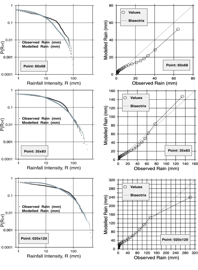
1 1 10 100 Rainfall Intensity, R (mm) Observed Rain (mm) Modelled Rain (mm) Point: 60x68 Point: 35x83 Point: 020x120

Fig. 9. Comparison of the rainfall intensities at sample points for July. Left:Exceedance probabilities.

average rainfall amounts differ markedly from each other, are maintained in the proposed model with reasonable accuracy.

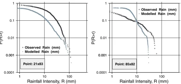
Although the model reproduces the intensity distributions which match observations in the rainy summer months, it performed less well in (less-rainy) winter months. (Fig. 10.). In addition to the intensity distribution at different locations, another important feature related to the intensity of spatial rainfall is the spatial correlation of rain quantities. For example, in the case of flood mitigation, an event with a high spatial autocorrelation and moderate peak intensities, can cause a more severe response than one with a higher peak intensity but a very low correlation. There are several methods to quantify the spatial autocorrelation. A measure

of spatial autocorrelation to study stochastic phenomena, distributed in space in two or more dimensions, is Moran’s I statistic, (Moran, 1950), which is used to quantify the correlation of the adjacent data in a matrix of n members. Moran’s I can be extended to incorporate variable lag-distance L (Sawada, 1999). In the present validation, the Moran’s statistic with a variable distance L was used. Figure 11 shows the I(L) functions for selected observed and modelled rain fields. For comparison, those for a ‘rainfall distribution’ based on a random field are also shown. Figure 11 indicates that the proposed multifractal-based approach can maintain the spatial structure of rainfall as well as the intensities.

Discussion

The objective of the proposed model is to preserve the spatial heterogeneity of spatial rainfall, in the multifractal modelling

process. If a multifractal model (β-lognormal model or any

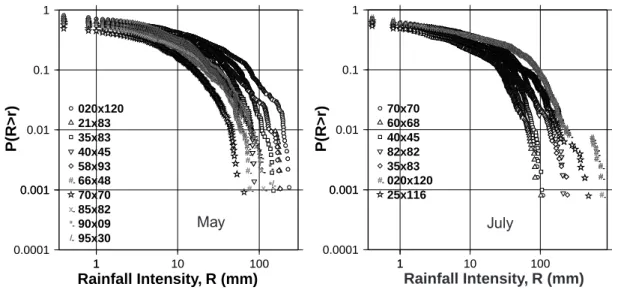
other spatial multifractal process) is used without any modification similar to that proposed in this paper, the statistical distribution of the ensemble of rainfall intensities at any location would be identical, so that information on the spatial heterogeneity would be lost. For example, in July, the exceedance probability curves for the points (20, 120), (35, 83) and (60, 68) would be identical, if an unmodified multifractal model were used. In reality, the intensities seen at those points are quite different. The proposed modified multifractal approach could capture that heterogeneity. The exceedance probability curves calculated from observed rainfall (R), of a number of locations are given in Fig. 12. Figure 13 shows the same for the modified field (M). The

modification M_i,j= R_i,j/G_i,jmakes the exceedance probabilities

of all the locations in the area, the same — a situation that

0.0001 0.001 0.001 0.01 0.1 1 P(R>r) 1 1 10 100 Rainfall Intensity, R (mm) Observed Rain (mm) Modelled Rain (mm) Point: 21x83 0.0001 0.001 0.001 0.01 0.1 1 P(R>r) 1 1 10 100 Rainfall Intensity, R (mm) Observed Rain (mm) Modelled Rain (mm) Point: 85x82

Fig. 10. Intensities for January. Though the long-term heterogeneity is maintained (Fig. 7, the model could not

capture the intensity variations properly.

-0.2 0 0.2 0.4 0.6 0.8 1 0 0.1 0.2 0.3 0.4 0.5 0.6 Distance L (Deg.) Moran's I R Observed R Modeled R with Random M

Fig. 11. Comparison of spatial correlations. (a) Observed: from the

rainfall snapshot of 01-Jul-1995. (b) Modelled data: A model-generated field with the large scale forcing as the average rainfall of 01-Jul-1995. (c) Random: The field computed for case b was randomly shuffled (correct intensities but no structure),

can be analysed as well as simulated successfully, using

multifractals. In simulating the inverse operation, R_i,j=

M_i,jG_i,jis applied to the fields generated by multifractal

simulation, so that they produce the intensity lineup similar to that given in Fig. 12.

The agreement of the intensity distributions, however, does not need a spatial structure similar to the rainfall snapshots. For example, even with a random distribution for M, the intensity distributions for R fields might be achieved. But, as indicated by the non-existent spatial autocorrelations in Fig. 11, a rainfall field R (= MG), based on a random M cannot maintain an adequate correlation

0.0001 0.001 0.001 0.01 0.1 1 1 1 10 100 # # ## ## ## ###################################################################################################################################################################################################################################################################################################################################################################################################################################_##### # # # ####_### # #_## # # # # # # # x x xx xx xx xx xxxxxxxxxxxxxxxxxxxxxxxxxxxxxxxxxxxxxxxxxxxxxxxxxxxxxxxxxxxxxxxxxxxxxxxxxxxxxxxxxxxxxxxxxxxxxxxxxxxxxxxxxxxxxxxxxxxxxxxxxxxxxxxxxxxxxxxxxxxxxxxxxxxxxxxxxxxxxxxxxxxxxxxxxxxxxxxxxxxxxxxxxxxxxxxxxxxxxxxxxxxxxxxxxxxxxxxxxxxxxxxxxxxxxxxxxxxxxxxxxxxxxxxxxxxxxxxxxxxxxxxxxxxxxxxxxxxxxxxxxxxxxxxxxxxxxxxxxxxxxxxxxxxxxxxxxxxxxxxxxxxxxxxxxxxxxxxxxxxxxxxxxxx_{xxxxxxxxxxxxxxxxxxx} x x x xx xx_{xxxxxxxxxxxxxxx} x x x xx_{xxxxxxxxxxxxx} x x x xxxxxxxxxxxx_xxxxx x xxxxxx_xxx x xxx_xx x x x x x x x x x ** ** _{** ** ** *********************************************} *****************************************************_{***********************************************************************} ********************************************************************* ********************************************************_{*********************************************} *******************************************_{***********************************} *************************_{********************} ****************_************ **********_******** *** ***_** **_* * ** ** ** * // _{// // // // // // ///////////} ////////////////////////////////////////////////////////_{///////////////////////////////////////////////////////} //////////////////////////////////////////////////////////////////////////////_{///////////////////////////////////////////////////////////////} ///////////////////////////////////////////_{//////////////////////////////////} ////////////////////////////////_{////////////////////////} //////////////////////_{//////////////// //} ////////////_//////// ////////_////// //// ////_// // // // // / 020x120 21x83 35x83 40x45 58x93 66x48 # 70x70 85x82 x 90x09 * 95x30 / Rainfall Intensity, R (mm) July P(R>r) Rainfall Intensity, R (mm) May P(R>r) 0.0001 0.001 0.001 0.01 0.1 1 1 1 10 100 # # ## ## #################################################################################################################################################################################################################################################################################################################################################################################################################################################################################################################################################################################################################################################################################################################################################################################################################################################################################################################_##### # ##_### # #_# ###_## # # # # # # # # # 70x70 60x68 40x45 82x82 35x83 020x120 # 25x116

Fig. 12. The observed exceedance probabilities for the months of May and July.

0.0001 0.001 0.001 0.01 0.1 1 0.01 0.10.1 1 10 # # ## ## #################################################################################################################################################################################################################################################################################################################################################################################################################################################################################################################################################################################################################################################################################################################################################################################################################################################################################################################_##### # ##_### # # # ###_## # # # # # # # # # 70x70 60x68 40x45 82x82 35x83 020x120 # 25x116 0.0001 0.001 0.001 0.01 0.1 1 0.1 0.1 1 10 # # ## ## ## ###################################################################################################################################################################################################################################################################################################################################################################################################################################_##### # # # ####_### # #_## # # # # # # # x x xx xx xx xxxxxxxxxxxxxxxxxxxxxxxxxxxxxxxxxxxxxxxxxxxxxxxxxxxxxxxxxxxxxxxxxxxxxxxxxxxxxxxxxxxxxxxxxxxxxxxxxxxxxxxxxxxxxxxxxxxxxxxxxxxxxxxxxxxxxxxxxxxxxxxxxxxxxxxxxxxxxxxxxxxxxxxxxxxxxxxxxxxxxxxxxxxxxxxxxxxxxxxxxxxxxxxxxxxxxxxxxxxxxxxxxxxxxxxxxxxxxxxxxxxxxxxxxxxxxxxxxxxxxxxxxxxxxxxxxxxxxxxxxxxxxxxxxxxxxxxxxxxxxxxxxxxxxxxxxxxxxxxxxxxxxxxxxxxxxxxxxxxxxxxxxxxxx_{xxxxxxxxxxxxxxxxxxx} x x x x x xx_{xxxxxxxxxxxxxxx} x x x xx_{xxxxxxxxxxxxx} x x x xxxxxxxxxxxx_xxxxx x xxxxx_x xxx_x xxx_xx x x x x x x x x x ** ** ** ** ** *********************************************_{*****************************************************} ***********************************************************************_{*********************************************************************} ********************************************************_{*********************************************} *******************************************_{***********************************} *************************_{********************} ****************_************ ********** ********_*** ***_** **_* * ** ** ** * // _{// // // // // // ///////////} ////////////////////////////////////////////////////////_{///////////////////////////////////////////////////////} //////////////////////////////////////////////////////////////////////////////_{///////////////////////////////////////////////////////////////} ///////////////////////////////////////////_{//////////////////////////////////} ////////////////////////////////_{////////////////////////} ////////////////////// //////////////////_//////////// ////////_//////// ////// //// ////_// // // // // / 020x120 21x83 35x83 40x45 58x93 66x48 # 70x70 85x82 x 90x09 * 95x30 /

Modified Rainfall Intensity, M (mm) July : with M=R/G

P(R>r)

Modified Rainfall Intensity, M (mm)

May : with M=R/G

P(R>r)

Fig. 13. The modification M=R/G, causes the exceedance probabilities to overlap. Only a few values at the

highest intensity show some scatter.

structure. This justifies the need for the multifractal component of the model.

INTENSITY DISTRIBUTIONS FOR WINTER MONTHS

The proposed method produced an acceptable representation of heterogeneity, as indicated by the long-term accumulations, for all the months of the year. However, the intensity distributions at locations with different heterogeneity were accurate only for the summer months. To explain the apparent reason for the mismatch of the distributions for the winter months, the relevant exceedance

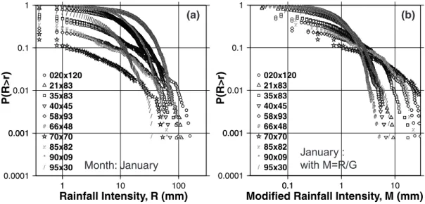
probability curves must be presented. Figure 14(a) shows the exceedance probability curves for a number of locations for January. The striking difference between this curve and those in Fig. 12 is that while the low intensity (high probability) end of the May and July curves almost coincide, those of the January curves are far apart; the spatial heterogeneity in summer rainfalls is caused mainly by the differences in (high) rainfall intensity while in winter it is caused largely by the difference in rainy periods (wet and dry periods). The intensity modification M/G takes care only of the rainfall quantity — an entity governed mainly by the occurrences of high intensities. On the other hand, the

multifractal model parameter β controls the wet fraction in

simulated rainfall snapshots. This is the parameter which determines the number of zero values in an integration of

intensities at a point, over time. In the proposed model, β is

not varied from place to place and hence the model cannot capture heterogeneity caused by differences in rainy fraction.

PREVIOUS WORK

Jothityangkoon et al. (2000) incorporated spatial heterogeneity in cascade modelling by introducing a heterogeneity term into the cascading process itself. They modified the cascade weight, W as W=L*G, where L is the cascade weight obtained from the multifractal generator, and

G is the heterogeneity term obtained by degenerating the

long-term average rainfall (on a monthly basis) to the appropriate cascade level. The authors have mentioned that there is a theoretical problem associated with the model. Though the introduction of the heterogeneity term (G) into the cascading process resulted in heterogeneous spatial fields

in the simulation, there was no way to use the reverse of this technique in data analysis. Jothityangkoon et al. (2000) used the parameter evaluation method proposed by Over and Gupta (1996) directly for data analysis. This led to a theoretical contradiction in the analysis and simulation phases, assuming rainfall to be a ‘pure’ cascade process in the analysis and a cascade process modified by a heterogeneity term in the simulation. This issue is important because the scaling properties of observed rainfall before and after the removal of heterogeneity are generally different. In addition to being simpler, the method proposed in the present study eliminates this inconsistency by treating the spatial heterogeneity separately from the multifractally represented random variability.

Another advantage of the present proposal is that it separates the multifractal modelling from the technique for handling heterogeneity, which simplifies the whole model. Further, such a separation makes it possible to use any multifractal scheme, including those which, in contrast to the present β-log normal model, do not use an explicit cascading process to represent the variability (M) in the model (e.g. ‘continuous’ multifractals introduced by Wilson

et al. (1991)).

Conclusions

A simple scheme to prevent the loss of spatial heterogeneity information during the process of multifractal modelling of spatial rainfall is proposed. The model involves filtering the observed rain fields to obtain data sets that are spatially homogeneous in a statistical sense. The spatial variability of these statistically homogeneous fields was used to fit a 0.0001 0.001 0.001 0.01 0.1 1 1 1 10 100 # # # ## ## ## #######################################################################################################################################################################################################################################################################################################################################################################################################################################################################################################################################################################################################################################################################################################################################################################################################################################################################################################################################################################################################################################################################################################################################################################################################_##### # # # ###_# ###_## # # # # # # # # # x x x_{x x} x xx xx xxxxxxxxxxxxxxxxxxxxxxxxxxxxxxxxxxxxxxxxxxxxxxxxxxxxxxxxxxxxxxxxxxxxxxxxxxxxxxxxxxxxxxxxxxxxxxxxxxxxx_{xxxxxxxxxxxxxxxxxxxxxxx} x xxxxxxxxxxxxxxxxxx_{xxxxxxxxxxxxx} x xxxxxxxxxxxx_xxxxxxxx xxxxxxxx_xxxxx x xxx_x xxx_xx x x x x x x x ** _{** ** ** ** ** ** *************************************************************************} **********************************************************************************_{**************************************************************************************************} ****************************************************************************************************************_{****************************************************************************************************************} ************************************************************** **********************************************************************_{****************************************************} ***************************************_{***************************************} ************************_{*********************} **************_{****************} **********_********** ******_**** **** ****_** ** ** ** ** * // _{// // // // // // /} / // ///////////////////// /////////////////////////////////_{///////////////////////////////////} //////////////////////////////////////////////_{////////////////////////////} /////////////////////////////////////////_{//////////////////////////////////////////} //////////////////////////////////_{//////////////////////////////} ////////////////////////_{//////////////////} //////////////_//////////// ////////_////// //////_//// ////_// // // // // / 020x120 21x83 35x83 40x45 58x93 66x48 # 70x70 85x82 x 90x09 * 95x30 / 0.0001 0.001 0.001 0.01 0.1 1 0.1 0.1 1 10 # # # ## ## #######################################################################################################################################################################################################################################################################################################################################################################################################################################################################################################################################################################################################################################################################################################################################################################################################################################################################################################################################################################################################################################################################################################################################################################################################_##### # ###_## # ###_## # # # # # # # # # x x x_{x x} x xx xxxxxxxxxxxxxxxxxxxxxxxxxxxxxxxxxxxxxxxxxxxxxxxxxxxxxxxxxxxxxxxxxxxxxxxxxxxxxxxxxxxxxxxxxxxxxxxxxxxxxxx_{xxxxxxxxxxxxxxxxxxxxxxx} x xxxxxxxxxxxxxxxxxx_{xxxxxxxxxxxxx} x xxxxxxxxxxxx_xxxxxxxx xxxxxxxx_xxxxx x xxx_x xxx_xx x x x x x x x ** _{** ** ** ** ** ***************************************************************************} **********************************************************************************_{**************************************************************************************************} ****************************************************************************************************************_{****************************************************************************************************************} **************************************************************_{**********************************************************************} ****************************************************_{***************************************} ***************************************_{************************} *********************_{**************} ****************_********** **********_****** **** ****_**** ** ** ** ** ** * // _{// // // // // // /} / /////////////////////// /////////////////////////////////_{///////////////////////////////////} //////////////////////////////////////////////_{////////////////////////////} /////////////////////////////////////////_{//////////////////////////////////////////} //////////////////////////////////_{//////////////////////////////} ////////////////////////_{//////////////////} //////////////_//////////// ////////_////// //////_//// ////_// // // // // / 020x120 21x83 35x83 40x45 58x93 66x48 # 70x70 85x82 x 90x09 * 95x30 / P(R>r) Rainfall Intensity, R (mm) Month: January

Modified Rainfall Intensity, M (mm)

January : with M=R/G

(a) (b)

P(R>r)

Fig. 14. Exceedance probabilities for the month of January. (a) Observed field, R. (b) Modified field, M

multifractal model. The simulation process was the exact opposite of the above; using the multifractal model, spatially homogeneous fields were simulated and later these were ‘modified’ to add the spatial heterogeneity. It was assumed that the spatial heterogeneity can be represented accurately by the normalised long-term average rainfall.

The model disaggregated the rainfall of Japan accurately and maintained at the simulation stage the large heterogeneity shown by the observations. However, the model did not produce the intensity distributions at different places accurately for the winter months because the heterogeneity of summer rainfall is caused mainly by differences in intensity while that of winter rainfall is due to the differences in rainy periods at different spatial locations. The present model can handle only the heterogeneity caused by the former situation.

References

Deidda, R., Benzi, R. and Siccardi, F., 1999. Multifractal modeling of anomalous scaling laws in rainfall. Water Resour. Res., 35, 1853–1867.

Gupta, V.K. and Waymire, E., 1990b. Multiscaling properties of spatial rainfall and river flow distributions. J. Geophys. Res.,

95, 1999–2009.

Jothityangkoon, C., Sivapalan, M. and Viney, N.R., 2000. Tests of a space-time model of rainfall in southwestern Australia based on nonhomogeneous random cascades. Water Resour. Res., 36, 267–284.

Lammering, B. and Dwyer, I., 2000. Improvement of water balance in land surface schemes by random cascade disaggregation of rainfall. Int. J. Climatol., 20, 681–695.

Lovejoy, S. and Mandelbrot, B.B., 1985. Fractal properties of rain, and a fractal model. Tellus, 37A, 209–232.

Makihara, Y., 1996. A method for improving radar estimates of precipitation by comparing data from radars and raingauges. J.

Meteorol. Soc. Japan, 74, 459–480.

Menabde, M., Seed, A., Harris, D. and Pegram, G., 1999. Multiaffine random field model for rainfall. Water Resour. Res.,

35, 509–514.

Meneveau, C. and Sreenivasan, K. R., 1987. Simple multifractal cascade model for fully developed turbulence. Phys. Rev. Lett.,

59, 1424–1427.

Moran, P.A.P., 1950. Notes on continuous stochastic phenomena,

Biometrika, 37.

Olsson, J., 1998. Evaluation of a scaling cascade model for temporal rainfall-disaggregation. Hydrol. Earth Syst. Sci., 2, 19–30.

Olsson, J. and Niemczynowicz, J., 1996. Multifractal analysis of daily spatial rainfall distributions. J. Hydrol., 187, 29–43. Over, T.M. and Gupta, V.K., 1994. Statistical analysis of mesoscale

rainfall: Dependence of a random cascade generator on large-scale forcing. J. Appl. Meteorol., 33, 1526–1542.

Over, T.M. and Gupta, V.K., 1996. A space-time theory of mesoscale rainfall using random cascades. J. Geophys. Res.,

101, 26,319–26,331.

Sawada, M., 1999. ROOKCASE: an excel 97/2000 visual basic (vb) add-in for exploring global and local spatial autocorrelation,

Bull. Ecol. Soc. Amer., 80, 231–234. url: http://www.uottawa.ca/

academic/arts/geographie /lpcweb /newlook/data_and_ downloads/download/sawsoft/rooks.htm.

Shuttleworth, W.J., 1988. Evaporation from Amazonian rainforest.

Proc. Roy. Soc. London Ser. B, 233, 321–346.

Tessier, Y., Lovejoy, S. and Schertzer, D., 1993. Universal multifractals: theory and observations for rain and clouds. J.

Appl. Meteorol., 2, 223–250.

Wilson, J., Schertzer, D. and Lovejoy, S., 1991. Continuous multiplicative cascade model of rain and clouds. In: Non-linear

variability in geophysics: Scaling and Fractals, D. Schertzer

and S. Lovejoy (Eds.). Kluwer, Dordrecht, The Netherlands. 185–207.