Lyman α observations as a possible means for the detection of the heliospheric interface

HAL Id: insu-02889809

https://hal-insu.archives-ouvertes.fr/insu-02889809

Submitted on 12 Mar 2021

HAL is a multi-disciplinary open access

archive for the deposit and dissemination of

sci-entific research documents, whether they are

pub-lished or not. The documents may come from

teaching and research institutions in France or

abroad, or from public or private research centers.

L’archive ouverte pluridisciplinaire HAL, est

destinée au dépôt et à la diffusion de documents

scientifiques de niveau recherche, publiés ou non,

émanant des établissements d’enseignement et de

recherche français ou étrangers, des laboratoires

publics ou privés.

Lyman α observations as a possible means for the

detection of the heliospheric interface

Eric Quémerais, Rosine Lallement, Jean-Loup Bertaux

To cite this version:

Eric Quémerais, Rosine Lallement, Jean-Loup Bertaux. Lyman α observations as a possible means for

the detection of the heliospheric interface. Journal of Geophysical Research Space Physics, American

Geophysical Union/Wiley, 1993, 98 (A9), pp.15199-15210. �10.1029/93JA01180�. �insu-02889809�

JOURNAL OF GEOPHYSICAL RESEARCH, VOL. 98, NO. A9, PAGES 15,199-15,210, SEPTEMBER 1, 1993

Lyman

Observations as a Possible Means for the Detection

of the Hellospheric

Interface

ERIC QUI•MERAIS,

ROSlNE

LALLEMENT,

AND JEAN-LouP BERTAUX

Service d'Adronomie du Centre National de la Recherche Scientifique, Verri&res le Buisson, France

We first smnmarize our current knowledge of the flow of interstellar H and He gas through

the solar system. Both come from the same direction, but the H velocity is 20 kin/s, whereas the He velocity is 26 km/s as recently determined by Ulysses, identical to the velocity found for the local interstellar cloud (LIC) as recently determined from absorption lines detected in the spectrum of nearby stars. This velocity difference may be assigned to the deceleration of H atoms

at the hellospheric interface through coupling with the partially ionized interstellar plasma. Seen

from the inner solar system, the Lyman c• emission pattern of H atoms (resonance scattering of solar photons) is quite compatible with a standard model including no interaction for H at the

heliopause and therefore cannot be used to characterize such an interaction. We investigate three other types of Lyman c• observations which could bear the signature of the heliopause. First, it is shown from Monte Carlo modeling of the interface perturbation that the Lyman c• line profile

(accessible through high resolution spectroscopy from Earth orbit) varies in a different way from

upwind to downwind direction, whether there is a perturbation or not at the heliopause. Indeed, some Prognoz data show such a behaviour, and the potential of planned future observations

is discussed (HST and SOHO). Second, since some interaction models predict a decrease of H density at heliopause crossing along the wind (or H increase when cruising upwind), the slope of

the radial antisolar Lyman c• intensity between 15 and 50 AU, characterized by % such as I ,.• k r '• ,

is computed for various models of H density. It is shown that (1) the value of '• recorded along downwind trajectories depends too much on solar parameters (radiation pressure and ionization) to be very useful to detect a departure from a standard model; (2) the value of -• along upwind

trajectories is much less sensitive to solar parameters but radiative transfer of Lyman c• in the

interplanetary medium must absolutely be taken into account for a correct interpretation; (3) if taken at face value, the value '• -- - 0.78 reported for Voyager data between 15 and 50 astronomical

units cannot be explained with any standard model, and calls for an increase of density somewhere

further upwind. A good fit is obtained with a doubling of the density at 54 astronomical refits (hydrogen wall), but this is not a unique solution. Finally, the use of Lyman c• intensity maps recorded at large distances (30 - 50 AU) is considered. The shape of the map is different when a

hydrogen wall is present, and this method is less prone to instrumental drift and solar Lyman c• changes than the preceding one. The first method works whatever is the distance of the heliopause, whereas the two others require observations from upwind region, not too far from the hellopause

(a few tens of astronomical units at most).

1. INTRODUCTION

The flow of H and He atoms through the solar system,

cal]ed the interstellar wind, is a result of the relative motion

of the Sun in respect to the surrounding interstellar mate- rial. Through resonance scattering of solar photons at H

Lyman a (121.6 nm) and He I 58.4 nm, one can observe

these atoms at a solar distance of • 0.5 to a few astronom-

ical units from spacecraft in Earth's orbit or cruising the inner solar system. This "interstellar glow" was predicted

by Blare and Fahr [1970] and measured

for the first time

in 1970 [Bertaux and Blareout,

1971; Thomas

and Krassa,

1971]. H atoms

are strongly

ionized

by charge

exchange

with

solar wind protons (the newly created

neutral is so fast that

it is no longer illuminated

by the solar Lyman a line) and

by EUV solar radiation (A < 91.2 nm), which accounts

for

about 20 % of the total ionization. The sky Lyman a pat-

tern as observed from 1 astronomical unit is characterized

by a smooth variation between a wide maximum region of intensity • 600 R and a minimum region in the opposite direction of about 200 R. The obvious interpretation is that the interstellar wind is coming from the region of maximum

Copyright 1993 by the American Geophysical Union. Paper number 93JA01180.

0148-0227/93/93JA-01180 $05.00

emission

(the upwind direction);

in the downwind

direction,

the ionization cavity carved by the sun is partially filled be-

cause of the high temperature of the interstellar gas. The use of a Hydrogen absorption cell on Prognoz 5 and 6

allowed to analyze the interplanetary Lyman a spectral line width and position, and to derive the temperature Too =

8000 :k 1000 K and the velocity Voo = 20 km/s of the in-

terplanetary

H gas flow [Bertaux

et al., 1985]. The upwind

intensity was compatible with a density "at infinity" noo = 0.065 cm -s .

The direction of the incoming H flow was found to be identical to the axis of the helium cone, present downwind as a result of gravitational focusing: ecliptic longitude A = 254 4- 3 ø, ecliptic latitude /• = 7 4- 3 ø, that is to say near

the ecliptic plane and (by coincidence)

near the direction

of

the galactic center.

Since the local interstellar matter is likely to be partially

ionized, the plasma flow of the interstellar wind will inter-

act with the solar wind plasma, with possibly a heliopause

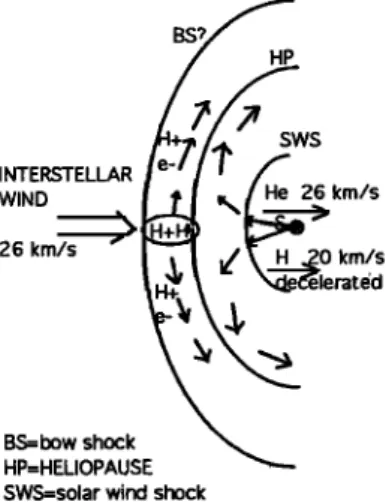
separating the two plasmas (Figure 1). The nose of the

heliopause, or the nearest point of interstellar matter un-

perturbed by the heliosphere is to be found in the direction

of the incoming interstellar wind. For further details on the modeling of the heliospheric interface, see, for example,

Holzer [1989], Barahoy

et al. [1991]

and Osterbart

and Fahr

[1992].

15,200 QUkMERAIS ET AL.: LYMAN c• DETECTION OF HELlOSPHERIC INTERFACE INTERSTELLAR WIND 26 km/s •' ELS=bow shock HP--HELIOPAUSE SWS:solar wind shock

Fig. 1. Schematic view of the heliospheric interface. Neutral

helium is unaffected while flowing through the diverted and de-

celerated plasma, as shown by the equality of velocity and tern- perature in the local cloud and within the heliosphere. Neutral H atoms distribution is likely to be affected by the plasma through

charge exchange with H + , and decelerated.

As suggested

by Wallis [1975], the interstellar plasma

(mainly protons and electrons)

may be decelerated

and de-

viated

by the heliospheric

obstacle

(Figure

1), and by H-H +

resonance charge exchange, the H neutrals are somewhat

coupled to the plasma. As a result, we do not know if the H parameters derived from Lyman a observation in the in-

her heliosphere

(noo,

Too,

Voo) are the interstellar

values

out

of the heliosphere, or if they represent only the gas inside

the heliosphere, after modifications at the hehospheric in- terface. On the contrary, neutral helium is very unlikely to

be affected by the plasma (Figure 1).

Several models of the neutral H interaction with the plas-

ma at the interface have been presen..ted and some of them

predict a decrease of the density, a decrease of the veloc-

ity and some heating. The case of a subcritical interstellar

flow has been considered

by Fahr and Ripken [1984], Os-

terbart and Fahr [1992], whereas

in the case

of a supersonic

two-shock model a Monte Carlo simulation of H atom trajec-

tories was performed

[Malama, 1991; Barahoy et al., 1991].

Different ways to infer quantitative estimates of the neu-

tral H perturbations

(mainly the deceleration)

have been

considered, as the comparison between the neutral solar system H and He velocities. One way is the comparison

between the "external" H velocity (the local interstellar gas

velocity),

and the "internal"

solar

sytem velocity

[Lallement

et al, 1986]. The local interstellar

cloud (LIC) is the name

given to the particular parcel of interstellar gas in which the sun is presently moving. Interstellar clouds can be detected

from their absorption lines recorded in high-resolution spec- tra of various stars, but up to now it had been impossible to tell if one particular observed absorption was due to the LIC or was due to a cloud further away, between the Sun

and the target star (or embedding

the target star), because

of the complexity

of the local gas [Lallement et al., 1986,

1990]. But, finally, the whole subject

became

suddenly

much

less speculative since the recent use of northern hemisphere high-quality observations which have led to the detection

of the LIC [Lallement and Bertin, 1992]. They analyzed

a series of ground-based high-resolution spectra of nearby stars emcmnpassing a wide portion of the sky, obtained at

Observatoire

de Haute Provence

(France), and derived the

velocity vector of VL,c of the local cloud, strongly confirmed

by one Hubble Space Telescope observation by Linsky et al.

[1992].

The direction

of l?L,c

motion

of the LIC respective

to the sun, (A = 74.9 + 30 , /• =-7.8 + 3ø), is nearly the

same as the direction of Voo, adding a new evidence that the

detected cloud was the local interstellar cloud. For further

details, see Bertin et al. [this issue].

However, the velocity was found to be 25.7 q- I km/s,

different from the 20 + I km/s observed

for H in the so-

lar system. But at the same time, Witte et al. [1992] re-

ported their Ulysses measurements of the flow of He atoms near Jupiter, by direct detection of impact of He atoms on

a litium fluoride target. See Witte et al. [1992] for a de-

tailed description of this new technique. They found that

the hehum flow through the solar system is characterized by

a velocity

vector

l•., (A = 72 q- 2.4

ø,/• =- 2.5 q- 2.7

ø) and

a

modulus

of 25.9

km/• that is to say

a vector

with the same

Therefore two things can now be concluded ß

1. The helium flow in the solar system is identical to

the motion of the LIC, proving that Hebron atoms are not

decelerated at the hehospheric interface.

2. If one refers to the most precise measurement of its velocity, the hydrogen flow is found to be decelerated by about 6 km/s, proving the existence of a strong interaction

near the heliopause.

The mere fact that the H flow inside the solar system

is found at 20 km/s instead of 26 km/s for Helium gives

an important clue to the effect of the heliospheric interface,

and in a sense this was recognized a long time ago, when

Dalaudier et al. [1984] had found, from optical measure-

ments of He 58.4 nm emission, a helium velocity of 27 q- 3

km/s. However, they had also found a rather large temper-

ature of He, not confirmed by Ulysses measurements, and

Chassefigre

et al. [1988] had given another

interpretation

of

the same measurements, in which the He velocity necessary

to fit the optical data could be pushed

down to 20 kin/s, if

the exciting solar line was itself strongly shifted. In fact, op-

tical measurements of He do suffer from a lack of accurate

knowledge of the solar hne, and the recent Ulysses direct

measurements put an end to this controversy.

In this paper, we examine how Lyman c• measurements

could bring more information on the distant region of in-

teraction, near the heliopause. As seen from the inner so- lar system, the Lyman c• intensity pattern can be perfectly represented by a standard "hot model," with no need to in-

voke anything special at the hehopause (with the inclusion

of some variations of the solar wind ionization rate with

latitude). But there are other types of measurements, ei-

ther with a refined analysis of the spectral profile of the backscattered Lyman c• hne, or intensity measurements at

large heliocentric distances, which may carry the imprint of

the interaction near the hehopause.

In the first section we review recent studies on the spectral

signature of the heliospheric perturbations in the hydrogen

glow. In particular, Monte Carlo simulations of H atoms trajectories, when taking into account the interaction with

the interstellar and solar plasmas before entering the he- liosphere, and the resulting Lyman a line shapes predicted

to be observed from I astronomical unit, show that these Lyman r• hne shapes have some peculiarities which do not

QU•MERAIS ET AL.' I.,YMAN C• DETECTION OF HELIOSP•E•tI½ INTERFACE 15,201

curate line shape measurements could bear the signature of

the heliospheric interface.

In the second section we analyze the behavior of antisolar Lyman c• intensity measurements as a function of the helio- centric distance r, in both downwind and upwind directions.

It is shown that downwind observations give a poor diag- nostic, because the effect of ionization can change in a large range the radial dependence of the intensity, whereas up- wind, an increase of density when going outside seems to fit Voyager observations presented by Gant7opadhgtagt and Judt7e

[1992]. A full model including radiative transfer of Lyman

a in the interplanetary space was build for this purpose. In the third section we examine the possibility to detect an increase of density from a sky map obtained at a large

distance

(30 or 45 astronomical

units) but still before

entering

the

region of increased density. Here again, a full model in- cluding the radiative transfer was used, which is absolutely

necessary to make correct predictions.

2. LYMAN a LINE PROFILES

2.1. Line Profiles in the Case of an Homogeneous Flow: Sensitivity to Interstellar and Solar Parameters

At present

(and within the next decade),

UV spectrome-

ters with a high enough resolution to measure the shape and

the Doppler shift of the Lyman a lines are (or will be) orbit- ing the Earth or within 2 astronomical units, and then we

will concentrate on the characteristics of the lines as viewed

from 1 astronomical unit. So close to the Sun, hydrogen

atoms are significantly affected by solar gravitation, radia-

tion pressure, and ionization, and the determination of the interstellar velocity Voo and temperature Too far from the

sun, (maybe already affected

by the interface), suffers

from

this complication, Within a few astronomical units, the bulk velocity is spatially dependent, and, due to the solar cycle

radiation and solar wind changes, it also varies with time. Resulting line profiles variations have been studied in the case of homogeneous flows approaching the Sun and opti-

cally thin radiation field [Wu and Judge, 1980; Lallement

et al., 1985]. The main solar effect remains the one of the

It parameter (ratio of Lyman a radiation pressure to grav-

itation). In the case of high, respectively

low, solar Lyman

a flux, H atoms are decelerated, respectively accelerated,

when approaching the Sun and then return to their initial velocity when moving away on the downwind side. It is in-

teresting to note that, even in the simple case where It is equal to 1 i.e., radiation pressure balances gravitation, if

all trajectories are straight fines with constant velocity for each atom, the bulk velocity is significantly changed both

in modulus and direction due to selection effects during the ionization processes (fast atoms, spending less time near the sun, are less ionized).

Fortunately, when using profiles measured toward differ- ent directions, it is possible to disentangle the profile char-

acteristics related to It from those related to the interstellar

parameters

• (v•elocity)

and

T (temperature)

far from

the

Sun and to measure these parameters independently, as was

done with the already mentioned hydrogen cell experiments.

This classical modeling of the Lyman a emission profile however, failed to explain the angular evolution of the emis-

sion profile when turning the direction of sight towards the downwind side as observed with Prognoz H absorption cell

in 1976-1977 [Bertaux et al., !985]. For more details see

Lallement [1990]. The discrepancies

between the upwind

and downwind observations suggest that the red part of the downwind line (reflecting H atoms leaving the heliospheric

cavity with the highest velocity) is enhanced

with respect

to what is expected from upwind profiles. This discrep- ancy has been attributed to different types of physical pro-

cesses.

The most probable

reasons

are; (1) departures

from

an homogeneous flow due to the hehospheric interface per-

turbations;

(2) multiple scattering

of Lyman t• photons;

(3)

time-dependent effects.

While in any case full radiative transfer line profile calcu-

lations and time-dependence inclusion are certainly neces- sary improvements of the models (indeed, radiative transfer codes have already been proven to change significantly at

least the intensity field, as shown in section 3, the first ex-

planation appears as the most appropriate, as we will show

below.

2.2. Quantitative Estimates of L•trnan o• Line Profiles

Variations Induced by Hellospheric Interface

One could imagine at first sight that the hydrogen flow having crossed the heliospheric interface is characterized by

a new distribution function, by comparison with the un- perturbed interstellar conditions, and that the first orders moments n, V, T of this distribution would be the same for

the rather small volume of gas illuminated by the Sun and contributing to the glow. In this case, one should be able to

determine these parameters n, V, T with the help of a clas- sical homogeneous flow model without interface; simply the

derived values would apply to the postinterface gas (and not to the initial interstellar flow), and we would have no sign at all of the initial conditions by looking at hydrogen only.

This is not true, for the very simple reason that the gas

which is detected along the stagnation hue on the upwind side and the gas which is detected on the downwind axis

do not come from the same direction: they have crossed

the interface in different regions characterized by different

plas•na properties, and then have started far from the Sun

with different distribution functions (Figure 1). In other

words, while they are at the same time rather close to the Sun in a small region, their history is different. This is due to the "umbrella effect" of the sun: schematically, H atoms able to reach the middle of the downwind cavity can not

come directly from the stagnation axis, since they would

have been ionized by the Sun, they come from the "sides,"

and they have crossed the flanks of the interface, where the

plasma is less decelerated and heated. It results that, de- pending on the direction the Lyman t• emission comes from,

one probes different initial properties of the emitting neu-

trals, i.e., different distribution characteristics the scatter-

ing neutrals had before approaching

the sun [Lallernent

and

Bertauac,

1990]. This gives a natural explanation

to the up-

wind to downwind profiles discrepancies discussed above,

provided the hydrogen distribution is significantly affected

by the interface.

To quantify this effect, which has the interesting prop- erty of being independent of the distance to the heliopause

and the shock(s),

two different approaches

have been used.

The first way is to start with an empirical inhomogeneous H distribution far frown the Sun, for which the velocity and temperature vary with the distance to the stagnation hue, to

model

all the flow

tubes

accordi•ng

to this

distribution,

and

15,202 QUgMmRAIS l•T AL.: LYMAN c• DI•TECTION OF HmMOSPHmR•½ INTERFACl•

The second way rehes on the computation of the upwind and

downwind line profiles for a full modelhug of plasma inter-

face and neutral H flow through the interface. This second approach requires an already fully developed plasma model. We will now describe these two approaches.

As we said, the H cell downwind observations of Prognoz

suggest that the red part of the downwind line is enhanced

with respect to what is expected from upwind profiles. The

existence of faster atoms is in agreement with the hypoth- esis that H is decelerated mostly along the stagnation line,

while atoms seen downwind have flown further away from

this line and are less decelerated. Qudmerais

et al. [1992]

have empirically modeled an axisymmetric hydrogen distri- bution whith the following characteristics: far from the Sun,

the initial bulk velocity and temperature is a function of the distance to the stagnation hue, as would result from the coupling with an axisymmetric plasma interface. Then all

atoms are followed during their travel through the heho-

spheric cavity, where they interact with the supersonic solar

wind only. Resulting hue profiles are computed, as well as the degree of absorption by a hydrogen cell, and the results are cronpared with observed Prognoz absorption rates. A

systematic search for the velocity and temperature depen-

dences on the distance to the stagnation hues which remove the best the previous homogeneous model discrepancies, is

then performed.

The results are interesting in the following way: they show

that, in order to fit the data, one has to increase the tem-

perature and decrease the bulk velocity along the stagnation

line, and inversely to decrease T•o and increase V•o on the

"sides". This corresponds qualitatively with the expected

modifications due to the physical processes at the interface.

However, quantitatively, the required velocity and tempera- ture modifications, are probably too large to be taken as real local values. As an example, the velocity decrease is of 16 km/s in the example shown in Figure 2, where the expected

and observed absorption rates by the H cell are displayed

along a scan plane perpendicular

to the ecliptic and nearly

parallel to the flow. Also, there is a range of directions- of-sight, not shown here, for which significant discrepancies remain. Then probably this kind of modehug is quantita-

tively too crude and some other effects are present.

The second approach is the use of the Baranov interface

model [Malama, 1991; Barahoy

et al., 1991],

coupled

with a

Monte-Carlo simulation of the neutrals flow through the in-

terface

[Malama, 1991],

to derive

the Lyman c• hue profiles

as

observed from the inner solar system. The main idea was to

quantify the upwind-downwind hue profiles evolutional pat- tern and to compare this angular evolutional pattern with

the no-interface

case [Lallement

et al., 1992]. As a matter

of fact, this is an observable quantity. In Figure 3 is shown the upwind emission hue profile resulting from the Baranov- Malama model. For more clarity we show a case where the interstellar proton density has the rather high value of 0.2

cm -a. A classical

homogeneous

model profile

is also shown,

for which interstellar parameters have been adjusted to pro- duce exactly the same profile as in the presence of the in-

terface. The two corresponding downwind profiles, at 180 ø from the previous direction, are shown in the same Figure. The profile which results from the full interface modelhug is very different from the "classical profile" with no interface. In this particular case used for demonstration the neutral H

is decelerated

by 13 km/s (from 29 to 16 km/s) along the

stagnation axis, while heated from 7600 K up to 12000 K. Along the sides, the velocity and temperature are less mod-

ified, being 21 km/s, and 9000 K respectively. Of course,

the variations decrease with the interstellar plasma density,

but it is interesting to note that there is still a detectable

difference

for 0.02 cm -a, which is a reasonable

value. This

proves that the umbrella effect is really significant, namely that even if the emitting H is confined within a rather small volume close to the sun, it comes from different portions of

1.00

• 0.96

• 0.92

• 0.88

i 0.72

• 0.68

ß

!' ' ,

O' PR(•GN0Z

DA+A:

se'ssion'l

...

I' ' '

--- INHOMOGENEOUS V--16 km/s at nose; 32 km/s on sides I - - - HOMOGENEOUS V=19 km/s everywhere ß ß ß ß

;ß

ß\

\

.,

N.__oos

\

o

o&,,

,,

o

=7,

o o z:o

-

Fig. 2. This figure is adapted from Qudmerais et al. [1992]. Absorptions by the prognoz H cell are best fitted by an inhomogeneous hydrogen flow entering the hellosphere, with slower and warmer atoms along the stagnation line, as compared with a classical homogeneous flow far t¾om the Sun. The data of session 1 were obtained for an Earth ecliptic longitude of 110 in a scan plane perpendicular to the Earth-Sun axis. The origin of the scan angle is deftned by the intersection of the scaa• plaam with the ecliptic plane, in the opposite direction of Earth motion.

QUkMERAIS ET AL.: LYMAN a DETECTION OF HELlOSPHERIC INTERFACE 15,203

14 '

' LY-[•_•..•_

LINE

PRO.••.• '

'

A H'OM OG N'•'•'-•O•-•' E (NO'•--•A) -

-•-- MONTE-CARLO THROUGH BARANOV INTERFACE

1 0.2 protons cm-3

IuP•-•ND

L-O-S

I

IoowNw,No

L-o•sl

1

i(

a

ß

- -

-60 -40 -20 0 20 40 60

KM/S (HELIOCENTRIC FRAME)

Fig. 3. This figure is adapted from Lalleraent et al. [1992]. The

Lyman c• line profile varies in a different way from upwind to downwind direction, wether there is a a perturbation or not at the hellospheric interface. Parameters have been adjusted to provide the same upwind profile.

the heliospheric interface. Therefore, by observing H Lyman

c• profiles, and their variations with direction of sight, one can learn something about the heliospheric interface.

œ.3. Past and Future Observations

œ.3.1. Spectroscopy. Spectra of the Lyman c• emission lines have already been observed directly by Adams and

Frisch [1976] with Copernicus

(OAO-3), at a resolution

of

about 15 km/s, resulting in a bulk velocity determination

of 22 4- 3 km/s, and later by Clarke et al. [1984] with IUE

at a resolution of 40 km/s, giving Vo• = 25.5 4- 5 km/s.

The line width being of the order of 15 km/s (full width

at half maximum), it is clear that the error bars are due

to the unfortunately too poor resolving power of the two instruments. The common interval 20.5-25 km/s for these two measurements is marginally compatible with the hydro- gen cell results 19-21 km/s on the upwind side. There were strong hopes associated with the Hubble Space Telescope

Goddard high resolution

spectrograph

(GHRS), which has

a resolving

power of 3 km/s in the Echelle Mode, and a pro-

posal has been accepted on this subject. The excellence of

the instrument and the feasiblity of such an accurate mea-

surement is largely proven by an observation obtained as a

by-product of early Mars observations

(J.L. Bertaux, pri-

vate communication,

1992). After 20 min of integration,

the interplanetary line is very well seen, showing that ex- posures of only 1 or two hours would have given very good

results. Unfortunately, the low-wavelength part of GHRS is

no longer operating at this high resolution, delaying further

measurements by an unknown number of years.

œ.3.œ. Hydrogen cell. The use of a hydrogen cell acting

as a kind of negative spectrometer, limited to the spectral

range implied by the spacecraft

(or Earth's) motion with re-

spect to the gas, but with infinite resolution, has been proven to bring very strong constraints on the line profiles. Indeed, the Prognoz H cell results are still a matter for analysis, as

has already been discussed above.

The future H cell experiment SWAN which should fly on

the solar and heliospheric

observatory

(SOHO) in 1995 for

2 years, has extended capabilities with respect to Prognoz,

providing

a full sky coverage

at any time (instead of a fixed

plan), and a better accuracy. It should provide extremely

strong constraints on the shapes and shifts of the lines, al-

lowing to measure the bulk velocities and to detect the de- partures from an homogeneous flow, when the hne of sight

moves from upwind to downwind. These departures, bear-

ing the signature of the heliospheric interaction, could help

describe the interface, whatever is its actual distance from

the sun.

3. RADIAL DEPENDENCE OF ANTISOLAR INTENSITIES

The outer-heliospheric spacecraft Voyager 1 and 2 and Pi-

oneer 10 and 11 provide us with new means to study the Ly- man a emissivity field in the hellosphere and then to get bet- ter constraints on the neutral hydrogen distribution in the heliosphere. Measurements of Lyman a intensities within

the inner heliosphere

(e.g., Prognoz 5/6, Pioneer-Venus...)

are more influenced by the solar environment and its ti•ne-

dependent or latitudinal variabilities, whereas such effects

are smoothed in the outer hellosphere.

Some studies from within the inner heliosphere have pro- vided a better understanding of the flow of interstellar hy-

drogen

[Lallement

et al., 1985; Chassefi•re

et al., 1986]. For

instance, the interstellar hydrogen number density has been

constrained between 0.05 and 0.2 cm -3. There are several

reasons for this rather large uncertainty. The illuminating Lyman a solar flux at line center varies; the same mea- sured intensity may correspond to different couples density

and ionization rate. Calibration factors evaluation may also

prove to be a difficult task and cause discrepancies between the results of different experiments. One way to rule out this

kind of problem is to study radial dependence of intensities

normalized to a chosen value.

On the other hand, as shown

by various

authors [Baranov

et al., 1991; Fahr, 1990], the hydrogen density distribution in the outer heliosphere may consistently differ from what is expected by a classical hot model, as developped for in-

stance

by Thomas

[1978]

or Lallement

et al. [1985]

described

by a uniform density at large distance from the Sun and a ionization cavity carved into it near the sun. Indeed, in the

case of an interface between interstellar and solar plasmas,

and since neutrals and protons are coupled through charge exchange processes, the hydrogen distribution in the outer heliosphere may differ greatly from the smooth distribution

obtained in the absence

of interface. Baranov et al. [1992]

give some possible H distributions according to computa- tions made with a Monte Carlo type model coupled with a plasma calculation. The main expected feature appears is the upwind direction. It consists of an important deple-

tion of neutral hydrogen along the stagnation line, near the position of the heliopause and the stagnation point of the

plasma distribution. The exact position of this feature is not

well constrained yet, neither is its exact shape. In fact, this sharp depletion feature may also be coupled with a slow ra- dial gradient of density between the Sun and the solar wind

shock.

Then, radial variations of backscattered Lyman c• intensi- ties provide us with a means to study this kind of problem. Since some of the spacecraft are now as far as 50 astronom- ical units from the sun, it is shown below that this problem

must not be studied by using the optically thin approxima-

tion and in what follows we have included radiative transfer

15,204 QU!•MERAIS ET AL.: LYMAN c• DETECTION OF HELlOSPHERIC INTERFACE

$.1. Density

Distribution

Model

With

no Interface

28

Our aim here is to study the radial variation

of antiso-

24

lar intensities

when

no interface

is considered.

Up to now

20

yields

wrong

conclusions

for this

problem.

16

In Figure

4 and 5, we show

the expected

H density

distri-

• 12

bution for some

given solar parameters.

The main feature

• 8

is a depletion around the Sun elongated in the downwind

direction

thus

leading

to quite

different

behaviours

in the

upwind

and downwind

directions.

The downwind

part of

õ-4

the cavity will be more or less depleted according to the o

a 8

value of the solar parameters. A greater lifetime of one H

•-12

atom at 1 astronomical

unit against ionization (Ta large),

as well as a stronger

focusing

effect

(It smaller

than 1) will

-16

tend to fill this cavity. Such distributions derived from the -20

classical hot model are relevant in the near-sun environment -24

(say within 20 astronomical

units from the sun) where ef-

-28

feets of an interface can be neglected. These distributions

are norInalized to the density "at infinity" noo which is one of the parameters of the model. It must be noted that if this parameter represents the density number in LIC for a no-interface model, in the case of an interface •nodel it rep- resents the number density after filtration by the interface.

Then, if the global effect of the interface is to divide the

nmnber density by a factor q along the stagnation line, the nmnber density in LIC is given by ntic = q

3.1.1. Optically

thin approximation. Let I(r-') be the an-

tisolar intensity measured at vector position •'. This quan-

tity can be computed according to the optically thin approx- imation by

I(r-')

= •

eot(•)

p(•r)

dr'

(1)

where p(w) is the nonisotropic

Lyman t• phase function

given

by Brandt

and Chamberlain

[19591

and Sot(;;)is

the

optically

thin emissivity

at r

-•. This value

is proportional

to

the H density

at • and to the solar Lyman a flux. Then

eot(• is proportional

to n(•')/r 2, from

which

we see

that, if

On/Or • O, I(• •nust be proportional

to 1/r.

It is obvious

from Figure 4 that the condition

On/Or • 0

will be fulfilled only far away from the Sun (say 15 astro-

nomical units in the upwind direction and 50 astronomical units downwind). Moreover since the density is an increas- ing function for increasing values of the distance from the

sun, at least for no-interface models, then the antisolar in-

tensity must fall off more slowly than 1/r which is typical of constant density. As we will see later this result is not true when multiple scattering is taken into account.

We must now take into account the fact that for a re-

alistic density distribution the density gradient is not zero

and depends on the interval on which it is cmnputed. In

what follows the radial dependence

of the intensity I(0 is

characterized by a coefficient 7 computed as the slope of a

linear function log(I) = 7 log(r)+ k. But as mentioned

before, the interval on which this approximation I • k r • is made will change the result. To avoid effects of the near-

solar environment, we have chosen distances greater than 15 astronomical units. Yet, in the downwind direction at 15 astronomical units from the Sun the effects of the cavity are

still rather important (Figure 4).

As an example, Table 1 displays the radial-dependence

coefficient

for three different

intervals ([15,501,

[50,1001

and

•, ...

T

d = 1 8 10

• s; [t = 0.7 i

':':':'"'"'"'

...

'•

....

'•,

...

i ...

ßi : .

I ...

':

...

';

...

0.7

...

':"%

...

:

...

ß

...

... ...

...

...

...

o ...

,, ...

...

...

...

,.:

.•

a'.. :""o

2':.;','/•.:

:•

'a-'i ...

'-v'"" ...

...

....

!

...

,"i

...

-7----'-io.

4.--,-:•

....

-'----'---•.--,•%'

...

:: ...

•

...

,---•

•' '• :'""'"•:'

':'"'• F

i ,

...

{

...

!.-

6

....

=,.,,:'::.•

...

• ...

i ...

, ...

+

...

...

zoos

I .... ,''';i' ''i .... i': :::l

-20 -10 0 10 20 •30

Astronomical Units

Fig. 4. Isodensity contours as expected from a classical hot model computed for two different sets of solar parameters. Upper

graph: Ta = 1.8 x 10 ½ s and tt = 0.7; lower graph: Td = 1.2 x 10 ½

s and tt = 0.7. The density is normalized to its value at large distalme from the sun. The direction of the incolning wind is shown by an arrow. The cavity is partly filled when Td increases

(less ionization by solar fluxes). This effect is •nore effective in

the downwind direction.

28 24 20 16 • 12 a 8 • 4

•-12

o.s ....

... ...

,:,,.,;:

...

!

....

o?...i

ß

•, - '_..':....'...'...."....'L'.

o. 4 ....

•.-•,-

.. X i o .,7 i

, i l

...

;.,:::Co'l

...

...-.,

...

,.,I

,.

½: ;i_'

N'f;I ! ....

,I

:'.:.

...

o' ...

...

...

''

: ,

:'"0.2 , ,'• :* ß :

.:1

-! i ! • ... "' i / i o.s'il - .•n c": ... !.•..•:...•.,.• ..'.--_=•,,'-' ... +..•. ...

'! i :

'! ...

i ...

T

d :

Fig. 5. Isodensity contours as expected frOIll a classical hot model computed for two different sets of solar parameters. The density is normalized to its value at large distance froin the

stm. Upper graph: Td = 1.2 x 10 • s and /• = 1; lower graph:

Td = 1.2 x 10 6 s and/• = 0.7. When/• increases, focalisation of

neutral atoms is less effective and the cavity is larger.

[15,100]) and three density

models

in the upwind and down-

wind directions. All models were computed for the same pa-

rameters

of the interstellar

wind (20 km/s and 8000 K). The

corresponding solar parameters are shown in Table 1. We

see from this Table that as the interval gets away from the Sun the coefficient tends toward the limit of-1, which means

QU!•MERAIS ET AL.: LYMAN • DETECTION OF HELIOSPHERIC INTERFACE 15,205

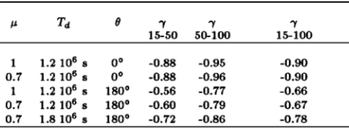
TABLE 1. Radial Dependence Coefficient Computed for Three Different Models in an Optically Thin Approximation

15-50 50-100 15-100 1 1.2 106 s 0 ø -0.88 -0.95 -0.90 0.7 1.2 106 s 0 ø -0.88 -0.96 -0.90 I 1.2 lO 6 s 180 ø -0.56 -0.77 -0.66 0.7 1.2 lO 6 s 180 ø -0.60 -0.79 -0.67 0.7 1.8 lO 6 s 180 ø -0.72 -0.86 -0.78

Outside 15 astronomical units, -• does not depend on the model in the upwind direction, whereas it is model-dependent in the downwind direction, according to the size of the downwind cavity.

quite true for the upwind direction which consequently show very little model dependence whereas the cavity effect is still rather important in the downwind direction even when the

lifetime against ionization of a H atom at 1 astronomical

unit is taken

rather

large

(1.8 x 106

s) which

tends

to fill the

downwind cavity.

It must be pointed out that if the radial dependence of in- tensity beyond 15 astronomical units observed by Pioneer 10

in the downwind

direction is equal to-1.07 [Gangopadhyay

and Judge, 1992], the use of the optically thin approxima-

tion leads us to the conclusion that the classical hot model

is inadequate to describe the downwind neutral distribu- tion beyond 15 astronomical units. Such a value suggests that the density in the downwind direction is fairly con-

stant (even decreases

a little with increasing

distance

from

the Sun) which cannot be obtained from hot models with

reahstic parameter values.

3.1.œ. Multiple scattering modelø For a temperature of 8000 K and far from the Sun, the H optical thickness per as- tronomical unit is of the order of the density "at infinity" n•

expressed

in cm

-3: r(1 AU)• n•(in cm-3), we see

that

the present positions of the outer heliospheric spacecraft do

not justify the use of an optically thin approximation

(O.T.).

A more complete modeling of radiative transfer for a res-

onance line must take two more effects into account. First,

a photon can be scattered •nany times and then contribute more than once to the emissivity field. Then, that there is extinction along the path of the photon which depends on its wavelength. The first effect tends to increase the real intensity respective to the O.T. approximation, whereas the second tends to decrease it; but these two effects do not compensate each other exactly.

In what follows, we have used a model developed by Qud-

metals and Bertau•c

[1992], which combines

a Monte Carlo

type code with a numerical code based on considerations similar to the work on the geocorona developped by Thomas

[1963] or Anderson and Hord [1977]. The main simplifica-

tions used in this work are complete frequency redistribution

(CFR) which, according

to Thomas

[1963] tends to slightly

overestimate the emissivity field, along with an isotropic emissivity function. The phase function expression given by

Brandt and Chamberlain

[1959] shows

that the maximum

discrepancy is of about 15 %, yet since here we are only in-

terested in gradients and not in absolute values the overall effect must be less important.

According to these assumptions, the antisolar intensity

can now be expressed as

&,

=

&

where a(t•) expresses

the spectral

dependence

of the absorp-

tion and scattering profiles and e -'v is the extinction along the line of sight. The emissivity field s(• takes multiple

scattering into account.

For Doppler profiles at the temperature of the gas (T• = $000 K), this expression becomes

1

s(•) T(r(• •) dr'

_,

(3)

where

r(•, r'] is the optical

thickness

at line

center

between

• and •' and T(r) is the Holstein

function

given

by

In this case the intensity gradient will depend on the be-

haviour of the extinction function represented

by T(r) and

of the emissivity

function e(r). Of course,

close to the Sun

the behaviour is similar to that of the optically thin approx- imation, yet for larger values of r the gradient becomes con- sistently different from what is expected from optically thin computations. In fact, extinction tends to become promi- nent over the multiple scattering effect which results in the

fact that for values of n• between 0.05 and 0.2 cm -3 the gradient is always steeper than what is expected from opti-

cally thin calculations: the denser the medium, the steeper the radial gradient of antisolar intensity.

The results of different computations have been summa- rized in Table 2. First, we see that the radial gradient can be steeper than -1 which is coherent with the fact that the opti- cally thin approximation overestimates the emissivity of far away points by neglecting extinction. We find also that for no-interface •nodels the upwind gradient is always steeper than the downwind gradient over the same intervals, simply because of the existence of the downwind cavity.

Gangopadhyay

and Judge [1992] have recently reported

that the Pioneer 10 data between 15 and 50 astronomical

units, exploring the downwind cavity, can be represented

with'a slope 7 = -1.07. They have claimed that this value, which is inco•npatible with any value obtained within the

TABLE 2. Radial Dependence Coefficient Computed for

Different Models With Radiative Transfer Calculations

• t d n• • • • • 15-50 50-100 15-100 1 1.2 0.1 0 ø -1.01 -1.36 -1.10 0.7 1.2 0.1 0 ø -1.03 -1.38 -1.11 I 1.2 O.1 180 ø -0.68 -1.20 -0.90 0.7 1.2 O.1 180 ø -0.71 -1.21 -0.91 0.7 1.8 0.05 180 ø -0.76 -1.13 -0.90 0.7 1.8 0.1 180 ø -0.85 -1.28 -1.01 0.7 1.8 0.15 180 ø -0.96 -1.36 -1.12 0.7 1.8 0.2 180 ø -1.03 -1.40 -1.18

All the models were computed for interstellar parameters 8000

K and 20 km/s. The solar parameters are indicated in the Table,

where td is the lifetime at I astronomical unit divided by one million seconds. 0 is the angle of the direction with upwind. The intervals used to compute -• are indicated. 0 = 0 ø corresponds to the upwind direction and 180 ø to the downwind direction.

15,206 QU!•MERAIS ET AL.: LYMAN • DETECTION OF HELIOSPHERIC INTERFACE

frame of the O.T. approximation and a standard hot model

(Table 1), was an evidence that the real downwind H den-

si.ty distribution was different from the standard model and called for a perturbation caused at the hehospheric bound- ary. It is interesting to note that it is however possible to obtain a coefficient 7 equal to the value given by the Pio- neer 10 data with the standard model though, in the frame-

work of radiative transfer model (last hne of Table 2), a

rather

large

number

density

noo

is required

(0.15-0.2

cm

-3)

as well as a large vMue for the hfetime at 1 astronomicM

unit (• 2 x 106 s) in order

to decrease

the size

of the down-

wind cavity. Taken alone, the downwind intensity gradient

is probably not a very good indicator of the effect of the

interface on the H density distribution.

3.œ. Density Distribution Model With Wall Type Interj'ace

In the previous paragraph we have shown that, beyond

15 astronomical units in the upwind direction, the radial dependence coefficient 7 was not very dependent on the solar parameters. Radiative transfer models give a value close to

-1 (see Table 2) on the interval 15-50 astronomical

units.

It is then interesting to compare such results with the Voyager 1 and Voyager 2 Lyman c• data. These data yield

a value of-0.7 for Voyager 1 and-0.78 for Voyager 2 [Hall

et al., 1993; Gangopadhyay

and Judge,

1992]. This seems

to

be in contradiction with a hot model with no interface and

these gradient values may be the signature of some jump of density lying ahead of the Voyager spacecraft which cruise

outwards near the upwind direction.

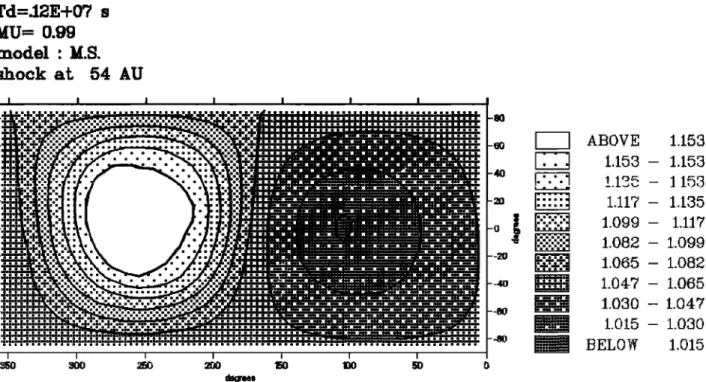
Since the imprint of a shock on the H neutrals is not well constrained yet, we have simply assumed that, at a given position in the upwind direction, the screening effect due to the interface could be represented by a jump in density.

Then, choosing one of the models of Figure 4 (/• = 0.99),

the number

density

factor noo

was taken equal to 0.2 cm

-3

for points with vMues of r > R• and with an angle with

the upwind direction

less than 40 ø and equal to 0.1 cm

-a

for all other points. The density distribution is shown in

Figure 6. At the position of the shock, the density is multi-

plied by 2 which is coherent with the results of Baranov et

al. [1991]. We tried three different values

for R•, 54 astro-

nomical units, 80 astronomical units and 107 astronomical units, to estimate find which position better agreed with the Voyager data.

In Table 3, we display the results of our computations for these density distributions. If the shock is at 54 astronomical units, the slope 7--0.78 is quite different froln the no-shock case at 7---1.01. The value of noo inside the shock is equal to

0.1 cln -a, which

means

that an optical

thickness

of 1 roughly

corresponds to 10 astronomical units. Therefore, from a vantage point at 50 astronomical units, only 4 astronomical

units (or r • 0.4) away from the H wall, it is not surprising

that the intensity is very much influenced by the presence of this wall. However, even if the H wall is at 80 astronomical

units, 7=-0.89 is significantly different from -1.01, in spite of

the optical thickness of 3 which separates the last observing position at 50 astronomical units and the H wall.

On the other hand, for radiative transfer computations,

the no-shock

model (which is equivalent

to R• = oo) and

the model with R• = 107 astronomical units show the same

gradient between 15 and 50 astronomical units. These two density distributions cannot be distinguished. The shock at 80 astronomical units modifies the gradient mainly for the

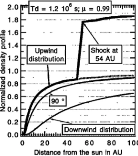
2.0 1.8 _.e 1.6 •.1.4 1.2 e0.8 •E0.6 z0,4 0.2 0.0

Td

= 1.2

10

e s;

It: 0.99

....

•

....

..•

Distance from the sun in AU

Fig. 6. Radial density distribution plotted for three different val- ues of 0, the angle with the upwind direction, in the case of a H

wMl. For 0 greater than 40 deg or r smaller then Rs (here Rs=54 astronomical units) we have a classical hot model with tz = 0.99,

Td = 1.2 x 106 s and noo=l (normalization), for 0 less than 40 ø

and r greater than Rs we take noo =2.

TABLE 3. Upwind Radial Dependence Coefficient With Shocks

ns in AU -y(15- 50) -y(15- 50)

Optically Thin Radiative Transfer

no shock -0.88 -1.01

107 -0.67 -0.99

80 -0.62 -0.89

54 -0.56 -0.78

Upwind radial dependence coefficient computed for four differ- ent density models, three of them with a shock at position Rs in the upwind direction. Optically thin and radiative transfer results are compared.

larger distances

in the interval [15 AU, 50 AU]. We must

realize also that, due to the important increase of the pri- mary emissivity in the shock region as compared to the no- interface case, points closer to the Sun than the shock have an increased secondary emissivity, due to photons backscat- tered from the shock region. Then the secondary emissivity

of the preshock region is increased as compared to the ex-

pected secondary emissivity in absence of the shock even if locally the density distributions are the salne. This higher secondary emissivity becomes a telltale sign of the shock, which may be itself too remote to be seen. We think this effect explains the fact that the gradient between 15 and 50 astronomical units is Inodified by a shock lying 30 astronom-

ical units beyond (that is roughly at an optical thickness of

3).

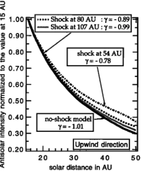
In Figure 7 we show the upwind antisolar intensities nor-

mahzed to the value at 15 astronomical units and computed for the four density distributions of Table 3. The effect of the existence and the position of the shock is quite clear, show- ing that in presence of a shock the intensity falls down less quickly than what is expected from a classical hot model.

It can be noted that the radial gradient given for Voy-

ager 2 (7=-0.78) is obtained

for a shock

at 54 astronomical

units (i.e. the density

is multiphed by 2 at 54 astronomical

units). As •nentioned above, this result is shghtly sensitive