HAL Id: cea-01135402
https://hal-cea.archives-ouvertes.fr/cea-01135402
Submitted on 25 Mar 2015
HAL is a multi-disciplinary open access
archive for the deposit and dissemination of
sci-entific research documents, whether they are
pub-lished or not. The documents may come from
teaching and research institutions in France or
abroad, or from public or private research centers.
L’archive ouverte pluridisciplinaire HAL, est
destinée au dépôt et à la diffusion de documents
scientifiques de niveau recherche, publiés ou non,
émanant des établissements d’enseignement et de
recherche français ou étrangers, des laboratoires
publics ou privés.
The XMM deep survey in the CDF-S
I. Georgantopoulos, A. Comastri, C. Vignali, P. Ranalli, E. Rovilos, K.
Iwasawa, R. Gilli, N. Cappelluti, F. Carrera, J. Fritz, et al.
To cite this version:
I. Georgantopoulos, A. Comastri, C. Vignali, P. Ranalli, E. Rovilos, et al.. The XMM deep survey in
the CDF-S. Astronomy and Astrophysics - A&A, EDP Sciences, 2013, 555, pp.A43.
�10.1051/0004-6361/201220828�. �cea-01135402�
DOI:10.1051/0004-6361/201220828
c
ESO 2013
Astrophysics
&
The XMM deep survey in the CDF-S
IV. Compton-thick AGN candidates
I. Georgantopoulos
1,2, A. Comastri
1, C. Vignali
3,1, P. Ranalli
2,1E. Rovilos
1,4, K. Iwasawa
5, R. Gilli
1, N. Cappelluti
1,
F. Carrera
6, J. Fritz
7, M. Brusa
3,1,10, D. Elbaz
8, R. J. Mullaney
8, N. Castello-Mor
6, X. Barcons
6, P. Tozzi
9,
I. Balestra
10, and S. Falocco
61 INAF – Osservatorio Astronomico di Bologna, via Ranzani 1, 40127 Bologna, Italy
e-mail: [email protected]
2 Institute of Astronomy & Astrophysics, National Observatory of Athens, Palaia Penteli, 15236 Athens, Greece 3 Physics & Astronomy Department, University of Bologna, Viale Berti Pichat 6/2, 40127 Bologna, Italy 4 Physics Department, University of Durham, South Road, Durham, DH1 7RH, UK
5 ICREA and Institut de Ciéncies del COSMOS (ICC), Universitat de Barcelona (IEEC-UB), Martí i Franqués 1, 08028 Barcelona,
Spain
6 Instituto de Fisica de Cantabria (CSIC-Universidad de Cantabria), 39005 Santander, Spain 7 INAF – Osservatorio Astronomico di Padova, Vicolo dell’Osservatorio 5, 35122 Padova, Italy 8 Irfu/Service Astrophysique, CEA-Saclay, Orme des Merisiers, 91191 Gif-sur-Yvette Cedex, France 9 INAF Osservatorio Astronomico di Trieste, via G.B. Tiepolo 11, 34143 Trieste, Italy
10 Max Planck für Extraterrestrische Physik, Karl Schwarzschild strasse, 85748 Garching, Germany
Received 30 November 2012/ Accepted 21 March 2013
ABSTRACT
The Chandra Deep Field is the region of the sky with the highest concentration of X-ray data available: 4 Ms of Chandra and 3 Ms of XMM-Newton data, allowing excellent quality spectra to be extracted even for faint sources. We took advantage of this to compile a sample of heavily obscured active galactic nuclei (AGN) using X-ray spectroscopy. We selected our sample among the 176 brightest XMM-Newton sources, searching for either flat X-ray spectra (Γ < 1.4 at the 90% confidence level) suggestive of a reflection dominated continuum or an absorption turn-over suggestive of a column density higher than ≈1024 cm−2. We found a
sample of nine heavily-obscured sources satisfying the above criteria. Four of these show statistically significant FeKα lines with large equivalent widths (three out of four have equivalent widths consistent with 1 keV) suggesting that these are the most certain Compton-thick AGN candidates. Two of these sources are transmission dominated while the other two are most probably reflection dominated Compton-thick AGN. Although this sample of four sources is by no means statistically complete, it represents the best example of Compton-thick sources found at moderate-to-high redshift with three sources at z= 1.2–1.5 and one source at z = 3.7. Using Spitzer and Herschel observations, we estimate with good accuracy the X-ray to mid-IR (12 µm) luminosity ratio of our sources. These are well below the average AGN relation, independently suggesting that these four sources are heavily obscured.
Key words.X-rays: diffuse background – infrared: galaxies – galaxies: active – X-rays: galaxies
1. Introduction
The nature of the X-ray background (XRB) has been contentious since its discovery 50 years ago (Giacconi et al. 1962). The Chandramission confirmed that the background is made up of the summed emission from active galactic nuclei (AGN;Brandt & Hasinger 2005). The resolved fraction of the XRB is about ∼90% in the 0.5–2 keV and 2–5 keV bands (Alexander et al. 2003;Xue et al. 2011). Optical spectroscopic follow-up obser-vations show that the peak of the redshift distribution of these sources is at z ∼ 0.7−1 (Barger et al. 2003; Silverman et al. 2010). At higher energies, the limited sensitivity hampers the resolution of a large fraction of the XRB. Narrow energy-band source stacking shows that this fraction reduces to ∼60% over 5−8 keV, and only ∼50% above 8 keV (Worsley et al. 2005,
2006;Xue et al. 2012;Moretti et al. 2012).
Still, it is at high energies where the bulk of the XRB en-ergy density is produced. The peak of the X-ray background at 20–30 keV (e.g.Frontera et al. 2007; Churazov et al. 2007;
Moretti et al. 2009) can be reproduced only by invoking a
significant number of heavily obscured and Compton-thick AGN. Compton-thick AGN are those where the absorbing col-umn densities exceed 1.5 × 1024 cm−2 and thus the
attenua-tion of X-rays by photoelectric absorpattenua-tion is enhanced by the scattering on electrons (for reviews on Compton-thick AGN properties and surveys see Comastri 2004; Georgantopoulos 2012). However, the exact density of heavily obscured AGN required by X-ray background synthesis models is still under dispute (Gilli et al. 2007; Sazonov et al. 2008; Treister et al. 2009a; Ballantyne et al. 2011; Akylas et al. 2012). In partic-ular, the intrinsic fraction of Compton-thick AGN may vary from 15 to over 35% (see discussion in Akylas et al. 2012). Additional evidence of a numerous Compton-thick population comes from the directly measured space density of black holes in the local Universe (see Soltan 1982). It is found that this space density is a factor of 1.5–2 higher than predicted by the X-ray luminosity function (Marconi et al. 2004; Merloni & Heinz 2008), although the exact number depends on the as-sumed efficiency in the conversion of gravitational energy to radiation.
The advent of the INTEGRAL and Swift missions helped to constrain the Compton-thick population in the local Universe. These missions explored the X-ray sky at energies above 10 keV probably providing the most unbiased samples of Compton-thick AGN over the whole sky. Owing to the limited imaging capabilities of these missions (carrying coded-mask detectors), the flux limit probed is bright ( f15−55 keV ∼ 10−11erg cm−2s−1),
allowing only the detection of AGN at very low redshifts. These ultra-hard surveys did not detect large numbers of Compton-thick sources (e.g.Ajello et al. 2008;Tueller et al. 2008;Paltani et al. 2008; Winter et al. 2009; Burlon et al. 2011; Malizia et al. 2012; Goulding et al. 2011). The fraction of Compton-thick AGN in these surveys does not exceed a few percent of the total AGN population. In contrast, optical and mid-IR sur-veys yield Compton-thick AGN fractions of between 10% and 20% (Akylas & Georgantopoulos 2009; Brightman & Nandra 2011). However, even the ultra-hard surveys may miss a fraction of Compton-thick AGN, i.e. those with NH > 2 × 1024 cm−2.
As Burlon et al. (2011) point out, this may explain the rel-ative scarcity of Compton-thick AGN found in the ultra-hard INTEGRAL and Swift surveys.
At higher redshifts, a number of efforts have been made to identify Compton-thick AGN. For example, Gilli et al. (2010) provide samples of Compton-thick AGN at moderate redshifts (z ∼ 1) using optical spectroscopy and in particular the [NeV] emission line. Searches for high-redshift Compton-thick AGN in the mid-IR also attracted much interest, mainly because the ab-sorbed radiation heats the surrounding material and is re-emitted at IR wavelengths. The techniques that have been employed in-clude the detection of a high 24 µm emission relative to the opti-cal emission (e.g.Fiore et al. 2008,2009;Georgantopoulos et al. 2008; Treister et al. 2009b; Eckart et al. 2010), and the pres-ence of a low X-ray-to-mid-IR luminosity ratio (seeAlexander et al. 2008,2011;Georgantopoulos et al. 2011b) Most recently,
Georgantopoulos et al. (2011a) proposed the presence of deep silicate features in mid-IR Spitzer spectra, although Goulding et al.(2012) argue that the silicate absorption in these sources is related to the host galaxies. Nevertheless, the most unambiguous method for finding Compton-thick sources relies on X-ray spec-troscopy. In X-ray wavelengths, the most systematic attempts in-clude these byTozzi et al.(2006);Georgantopoulos et al.(2007,
2009), and more recentlyBrightman & Ueda (2012) all in the Chandradeep fields. A number of Compton-thick sources have been individually discussed in Norman et al. (2002),Iwasawa et al.(2005),Comastri et al.(2011),Feruglio et al.(2011),Gilli et al.(2011),Georgantopoulos et al.(2011b), andIwasawa et al.
(2012a). In particular, Comastri et al.(2011) has provided the most direct X-ray spectroscopic evidence yet for the presence of Compton-thick nuclei at high redshift, reliably identifying two Compton-thick AGN at z= 1.536 and z = 3.700.
Here, we attempt to find unambiguous examples of Compton-thick AGN at moderate redshifts, extending the work of Comastri et al. (2011). The Chandra Deep Field South (CDF-S) is one of the regions of the sky with the largest ac-cumulation of multi-wavelength data available. In particular, it is the area with the most sensitive X-ray observations, namely 3 Ms of XMM-Newton data and 4 Ms of Chandra data, al-lowing the extraction of good quality X-ray spectra even for faint X-ray sources such as heavily obscured AGN. Owing to the superior XMM-Newton photon collecting power, we first select a sample of heavily obscured AGN using the 3 Ms XMM-Newton observations. For these sources, we present a combined XMM-Newton and Chandra spectral analysis to increase the photon statistics. Our aim is to detect unambiguous
signs of Compton-thick obscuration, such as direct detection of a large column density, or a flat spectral index, and finally a large equivalent-width (hereafter EW) Fe Kα line. Finally, we examine the mid-IR and far-IR (up to rest-frame wavelengths of 160 µm) properties of our sources using data from the Spitzer and Herschel missions. The aim is to check whether the IR ob-servations independently support a heavy obscuration scenario. We adopt Ho = 75 km s−1Mpc−1,ΩM = 0.3, and ΩΛ = 0.7
throughout the paper.
2. Data
2.1. X-ray
2.1.1. XMM-Newton
The CDF-S area was surveyed with XMM-Newton during di ffer-ent epochs spread over almost nine years. The data presffer-ented in this paper were obtained by combining the observations awarded to our project and observed between July 2008 and March 2010 (Comastri et al. 2011) with the archival data acquired in the period July 2001–January 2002. The total exposure time, af-ter the removal of background flares, is ≈2.82 Ms for the two MOS and ≈2.45 Ms for the PN detectors. The total area cov-ered is 30 × 35 arcmin. The source catalogue contains 339 X-ray sources detected in the 2–10 keV band with a significance larger than 5σ and a flux density limit of ≈6.6 × 10⁻¹⁶ erg cm−2s−1
assumingΓ = 1.7. A supplementary list of 74 sources detected with lesser significance is also provided. An extended and de-tailed description of the full data set, including data analysis and reduction and the X-ray catalogue, will be published inRanalli et al.(2013).
2.1.2. Chandra
The CDF-S 4 Ms observations consist of 53 pointings obtained in the years 2000 (1 Ms), 2007 (1 Ms), and 2010 (2 Ms). The analysis of the first 1 Ms data is presented in Giacconi et al.
(2002) andAlexander et al. (2003), while the analysis of the 23 observations obtained up to 2007 is presented inLuo et al.
(2008). In the present 4 Ms survey, 740 sources are detected down to a sensitivity limit of ∼0.7 × 10⁻¹⁶erg cm−2s−1 and
1 × 10⁻¹⁷erg cm−2s−1in the hard (2–8 keV) and soft (0.5–2 keV) band, respectively (Xue et al. 2011). The Galactic column den-sity towards the CDF-S is 0.9 × 1020cm−2(Dickey & Lockman
1990).
2.2. Infrared 2.2.1. Spitzer
The central regions of the CDF-S were observed in the mid-IR by the Spitzer mission as part of the Great Observatories Origins Deep Survey (GOODS). These observations cover areas of about 10 × 16.5 arcmin2 using the IRAC (3.6, 4.5, 5.8, and 8.0 µm) bands. These data are combined with more recent observations of the wider E-CDF-S area in the SIMPLE survey (Damen et al. 2011). The combined data-set has a 5σ magnitude limit of [3.6 µm] AB= 23.86, while the 3σ magnitude limit of the central GOODS region is [3.6 µm]AB= 26.15. The GOODS area in the centre of the CDF-S has also been imaged with the
MIPS detector onboard Spitzer in the 24 µm band with a 5σ flux density limit of 30 µJy. A much wider area, including the en-tire E-CDF-S was imaged as part of the FIDEL legacy program (Magnelli et al. 2009) with a 5σ flux density limit of 70 µJy; we use a combination of the two data-sets for this work.
2.2.2. Herschel
The far-Infrared data in this work come from the GOODS-Herschel survey of Elbaz et al.(2010). This is the deepest sur-vey of Herschel using the PACS instrument in both the 100 and the 160 µm bands, with an integration time of more than 15 h per position. The area covered is a 13 × 11 arcmin field in-side the GOODS area. The source detection is performed using a 24 µm prior position and the 3σ flux density limits are 0.8 and 2.4 mJy in the 100 and 160 µm bands respectively. The GOODS-Herschel catalogue we use also utilises public data from the HerMES survey (Oliver et al. 2012) in the CDF-S. We use a 250 µm catalogue based on 24 µm prior positions covering the GOODS-S area, and we keep sources with a flux density deter-mination better than the 2σ limit of 3.5 mJy.
3. Sample definition and X-ray spectral extraction
3.1. The sample
We confine our analysis to the brightest sources in the prelimi-nary XMM-Newton catalogue, i.e. those with a detection proba-bility of 8σ. There are 194 sources from both the main and sup-plementary lists satisfying the above criterion. However, for a number of sources we cannot derive an XMM-Newton spectrum in any of the cameras, either because they are too faint (they lie in areas of elevated background or low exposure) or they are confused. The number of confused sources is determined us-ing the Chandra imagus-ing. Therefore, the number of extracted spectra is 176. We match the XMM-Newton positions with the Chandrapositions using a radius of 5 arcsec, and find counter-parts for all 176 sources in the 4 Ms catalogue of Xue et al.
(2011) or the E-CDF-S catalogue ofLehmer et al.(2005). We build the multi-wavelength catalogue using all the in-formation available and the likelihood ratio method to select the counterparts, using the positional uncertainties provided in the various catalogues. We first combine the SIMPLE catalogue with both the K-selected (Taylor et al. 2009) and the BVR-selected (Gawiser et al. 2006) MUSYC catalogues (preferring K-selected sources where they are detected in both catalogues). We find the optical-infrared counterparts of the X-ray sources, constraining their positions, and then we look for counterparts in the FIDEL and 24 µm-prior Herschel catalogues.
Out of our 176 sources with Chandra counterparts, 136 have a spectroscopic redshift determination inSzokoly et al.(2004),
Le Fèvre et al. (2005),Norris et al. (2006),Ravikumar et al.
(2007),Vanzella et al. (2008),Treister et al.(2009a),Balestra et al.(2010),Silverman et al.(2010), andCooper et al.(2012). For 38 of the remaining sources, photometric redshifts have been compiled from Cardamone et al.(2010), Taylor et al.(2009),
Rafferty et al.(2011),Luo et al.(2010), andDahlen et al.(2010), while two sources have no redshift determination because they are too faint in optical – near-Infrared wavelengths.
3.2. XMM-Newton spectra
For each individual XMM-Newton orbit, source counts were col-lected from circular regions with radii between 10 and 25 arcsec, depending on field crowdedness and source brightness, and cen-tred on the 2–10 keV source positions. These radii correspond to encircled energy fractions of 59% and 86%, respectively consid-ering the on-axis XMM-Newton PSF at an energy of 4.2 keV (the average energy of a source with a spectrum ofΓ = 1). The encir-cled energy fraction does not change abruptly with the off-axis angle or the average energy. The above fractions become 55 and 80% at an off-axis angle of 9 arcmin and for an energy of 6 keV. Local background data were taken from nearby regions, sepa-rately for the PN, and MOS detectors to account for local back-ground variations and chip gaps, and to avoid XMM-Newton or Chandra detected sources. The areas of the background re-gions have on average 20 arcsec radii. The spectral data from individual exposures were summed for the source and back-ground, respectively, and a background subtraction was made assuming a common scaling factor for the source/background geometrical areas. Both the PN and the MOS spectra are ex-tracted in the 0.5−8 keV energy area. The MOS-1 and MOS-2 spectra are summed separately using the FTOOLS MATHPHA task. Response and effective area files were computed by av-eraging the individual files using the FTOOLS ADDRMF and ADDARFtasks.
3.3. Chandra spectra
We used the SPECEXTRACT script in the CIAO v4.2 software package to extract the spectra of Chandra sources. The extrac-tion radius varies between 2 and 4 arcsec with increasing o ff-axis angle. At low off-ff-axis angles (<4 arcmin), this area encircles 90% of the light at an energy of 1.5 keV. The same script extracts response and auxiliary files. The addition of the spectral files was performed with the FTOOL task MATHPHA. To add the re-sponse and auxiliary files, we used the FTOOL ADDRMF, and ADDARF tasks respectively, weighting according to the number of photons in each spectrum.
4. X-ray spectral fittings and selection method
The goal was to identify heavily obscured AGN via X-ray spec-tral analysis. We used the XSPEC v12.5 software package for the spectral fits (Arnaud 1996). We employed the C-statistic tech-nique (Cash 1979), which had been specifically developed to ex-tract spectral information from data of low signal-to-noise ratio. This statistic works on un-binned data, allowing us, in princi-ple, to use the full spectral resolution of the instruments with-out degrading it by binning. We perform our initial selection in the XMM-Newton data both because of its high effective area at high energies as well as for its good counting statistics. We fit the XMM-Newton spectra using the absorbed power-law model PLCABS (Yaqoob 1997). The advantage of the PLCABS model is that it properly takes into account Compton scattering up to column densities of NH∼ 5 × 1024cm−2.
Our selection method is summarised in the following criteria:
1) The detection of an absorption turnover corresponding to a column density of NH > 1.5 × 1024 cm−2. For a mildly
Compton-thick source with a column density ∼1024 cm−2, the absorption turnover occurs at rest-frame energies some-what higher than ∼8 keV. This implies that even with the
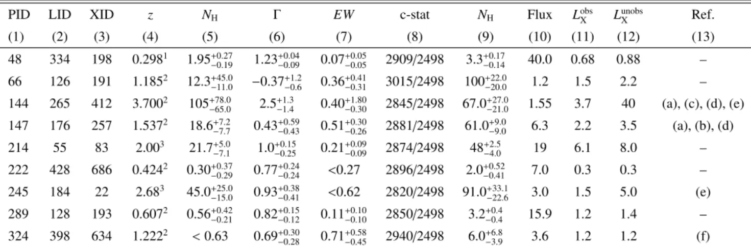
Table 1. Initial selection of Compton-thick candidates based on XMM-Newton absorbed power-law, (PLCABS), spectral fits.
PID LID XID z NH Γ EW c-stat NH Flux LobsX L
unobs X Ref. (1) (2) (3) (4) (5) (6) (7) (8) (9) (10) (11) (12) (13) 48 334 198 0.2981 1.95+0.27 −0.19 1.23+0.04−0.09 0.07+0.05−0.05 2909/2498 3.3+0.17−0.14 40.0 0.68 0.88 – 66 126 191 1.1852 12.3+45.0 −11.0 −0.37+1.2−0.6 0.36+0.41−0.31 3015/2498 100+22.0−20.0 1.2 1.5 2.2 – 144 265 412 3.7002 105+78.0 −65.0 2.5+1.3−1.4 0.40+1.80−0.30 2845/2498 67.0+27.0−21.0 1.55 3.7 40 (a), (c), (d), (e) 147 176 257 1.5372 18.6+7.2 −7.7 0.43+0.59−0.43 0.51+0.30−0.26 2881/2498 61.0+9.0−9.0 6.3 2.2 3.5 (a), (b), (d) 214 55 83 2.003 21.7+5.0 −7.1 1.0+0.15−0.25 0.21+0.09−0.09 2874/2498 48+2.5−4.0 19 6.1 8.0 – 222 428 686 0.4242 0.30+0.37 −0.29 0.77+0.24−0.24 <0.27 2896/2498 2.0+0.52−0.41 7.0 0.3 0.3 – 245 184 22 2.683 45.0+25.0 −15.0 0.93+0.38−0.41 <0.62 2820/2498 91.0+33.1−22.6 3.0 1.5 5.0 (e) 289 128 193 0.6072 0.56+0.42 −0.21 0.82+0.15−0.12 0.11+0.10−0.10 2850/2498 3.2+0.4−0.4 15.9 1.2 1.4 – 324 398 634 1.2222 < 0.63 0.69+0.30 −0.28 0.71+0.58−0.45 2940/2498 6.0+6.8−3.9 3.6 1.2 1.2 (f)
Notes. The columns are: (1) XMM-Newton ID. (2) Chandra ID fromLuo et al.(2008). (3) Chandra ID fromXue et al.(2011). (4) Redshift; two or three decimal digits denote X-ray or spectroscopic redshift, respectively; references:(1)Balestra et al.(2010),(2)Szokoly et al.(2004),(3)X-ray
redshift from current work. (5) NHcolumn density in units of 1022cm−2. (6) Photon index. (7) FeKα equivalent-width in units of keV; the energy
of the line has been fixed at a rest-frame energy of 6.4 keV. (8) c-statistic value/degrees of freedom. (9) Column density in units of 1022cm−2. for
a photon-index fixed atΓ = 1.8. (10) 2–10 keV flux in units of 10−15erg cm−2s−1. (11) 2–10 keV obscured luminosity in units of 1043erg s−1.
(12) Unobscured luminosity (estimated by removing the absorption component) in units of 1043 erg s−1. The flux and luminosities are derived
leavingΓ free. (13) previous X-ray reference: (a)Tozzi et al.(2006); (b)Georgantopoulos et al.(2007); (c)Norman et al.(2002); (d)Comastri et al.(2011); (e)Iwasawa et al.(2012a); (f)Georgantopoulos et al.(2011b). All errors refer to the 90% confidence level.
relatively large effective area of XMM-Newton at high en-ergies, it is difficult to detect the absorption turnover for marginally Compton-thick sources at low redshift. However, at higher redshifts the turnover shifts progressively to low energies making the identification of Compton-thick AGN more straightforward (Iwasawa et al. 2012b). For example, for a Compton-thick source with a column density of NH∼
1024 cm−2, the absorption turnover would shift to energies
about 2 keV at a redshift of z= 2, an energy region where XMM-Newton has large effective area. At a column density of 5 × 1024 cm−2, the turnover occurs at an energy of about 20 keV (e.g.Yaqoob 1997). This criterion is reliable only in the case of sources with a spectroscopic redshift available be-cause the rest-frame energy of the absorption turnover (and hence the exact value of the column density) requires knowl-edge of the redshift with high precision.
2) The detection of a flat spectral indexΓ < 1.4 at a statisti-cally significant level (90% confidence), i.e. the 90% upper limit of the photon index should not exceedΓ = 1.4. This is an arbitrarily selected, albeit extremely conservative, cut-off. The average photon index of AGN ranges between 1.7 and 2.0 with a standard deviation as low as 0.15 (e.g.Nandra & Pounds 1994;Dadina 2008;Brightman & Nandra 2011;
Ricci et al. 2011;Burlon et al. 2011). Therefore, a flat spec-trum may be characteristic of heavily obscured, reflection-dominated Compton-thick AGN (George & Fabian 1991;
Matt et al. 2004). We note however, that because of spec-tral degeneracy, it is likely that some sources appear to have flat spectra simply because of moderate (∼1022−23cm−2)
ab-sorption (see alsoCorral et al. 2011). This degeneracy is pro-nounced in sources with low signal-to-noise spectra. 3) For the sources which are selected according to the above
two criteria, we examine whether the addition of a Gaussian component is required by the data. This additional criterion is motivated by the fact that strong FeKα lines are often ob-served in Compton-thick AGN in the local Universe (e.g.
Fukazawa et al. 2011).
5. The Compton-thick candidates
5.1. XMM-Newton results
The XMM-Newton spectral fittings yield nine sources with ei-ther a flat spectrum1or a absorption turnover corresponding to a rest-frame column density greater than NH ≈ 1024 cm−2. The
XMM-Newton spectral fits (PLCABS + GA in XSPEC notation) of these nine sources are given in Table1. Eight, out of nine Compton-thick candidates, have a spectroscopic redshift avail-able. One out of those (PID-245) has a noisy optical spectrum and a highly uncertain spectroscopic redshift (1.864) based on only one line (Balestra et al. 2010). For this source there are also three photometric redshifts available 2.28, 2.43 and 3.0, (Dahlen et al. 2010;Santini et al. 2009;Luo et al. 2010), respectively. However, it is possible that the X-ray source does not correspond to the counterpart with the available optical spectrum (located 1 arcsec away).Iwasawa et al.(2012b) detect an FeKalpha line which corresponds to a redshift of z= 2.68. We chose to use this redshift instead of the optical ones. At this X-ray redshift there is no obvious optical lin
For source PID-214, for which there are only photometric redshifts available, z = 1.5 and z = 1.17 (Cardamone et al. 2010), there is a hint for a line at an energy of E= 2.13+0.04−0.03keV with EW = 0.3 ± 0.1 keV. On the basis of this line, assuming it is related to the FeKα at 6.4 keV rest-frame energy, the implied redshift would be z= 2.00 ± 0.05. Hereafter, we adopt the X-ray redshift for this source.
At least one source (PID-144) at a spectroscopic redshift of z = 3.70 is a probable transmission dominated Compton-thick source, i.e. it is characterised as Compton-thick on the basis of an absorption turn-over in its X-ray spectrum. This source was first reported as Compton-thick byNorman et al.(2002). A 1 In addition, there are two more sources which appear to have flat
spectra, but instead the 90% upper limits of their photon indices are just above the chosen threshold ofΓ = 1.4. These are sources PID-64 and PID-252 at a spectroscopic redshift of z= 0.516 and 1.893, respectively.
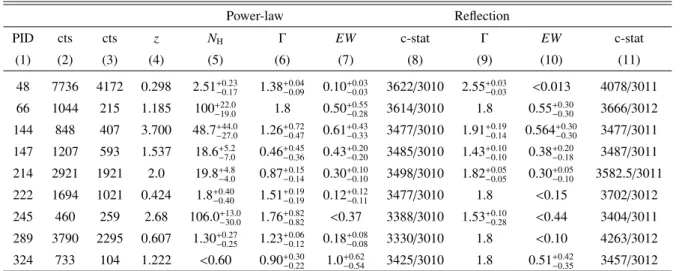
Table 2. Joint XMM and Chandra spectral fits of the full sample of Compton-thick candidates.
Power-law Reflection
PID cts cts z NH Γ EW c-stat Γ EW c-stat
(1) (2) (3) (4) (5) (6) (7) (8) (9) (10) (11) 48 7736 4172 0.298 2.51+0.23−0.17 1.38−0.09+0.04 0.10+0.03−0.03 3622/3010 2.55+0.03−0.03 <0.013 4078/3011 66 1044 215 1.185 100+22.0−19.0 1.8 0.50+0.55−0.28 3614/3010 1.8 0.55+0.30−0.30 3666/3012 144 848 407 3.700 48.7+44.0−27.0 1.26+0.72−0.47 0.61+0.43−0.33 3477/3010 1.91+0.19−0.14 0.564+0.30−0.30 3477/3011 147 1207 593 1.537 18.6+5.2−7.0 0.46+0.45−0.36 0.43+0.20−0.20 3485/3010 1.43+0.10−0.10 0.38+0.20−0.18 3487/3011 214 2921 1921 2.0 19.8+4.8−4.0 0.87+0.15−0.14 0.30+0.10−0.10 3498/3010 1.82+0.05−0.05 0.30+0.05−0.10 3582.5/3011 222 1694 1021 0.424 1.8+0.40−0.40 1.51+0.19−0.19 0.12+0.12−0.11 3477/3010 1.8 <0.15 3702/3012 245 460 259 2.68 106.0+13.0−30.0 1.76+0.82−0.82 <0.37 3388/3010 1.53+0.10−0.28 <0.44 3404/3011 289 3790 2295 0.607 1.30+0.27−0.25 1.23−0.12+0.06 0.18+0.08−0.08 3330/3010 1.8 <0.10 4263/3012 324 733 104 1.222 <0.60 0.90+0.30−0.22 1.0+0.62−0.54 3425/3010 1.8 0.51+0.42−0.35 3457/3012
Notes. The columns are: (1) XMM-Newton ID. (2) Net XMM-Newton counts (all three modules). (3) Net Chandra counts. (4) Redshift; two or three decimal digits denote photometric or spectroscopic redshift respectively. (5) NHcolumn density in units of 1022cm−2. (6) Photon index.
(7) Equivalent-width in units of keV; the energy of the line has been fixed at a rest-frame energy of 6.4 keV. (8) c-statistic value/degrees of freedom. (9) Photon-index for the PEXRAV model. (10) Equivalent-width of the FeKα line in the PEXRAV model. The line energy is fixed to 6.4 keV. (11) c-statistic value/degrees of freedom. All errors refer to the 90% confidence level.
much higher quality X-ray spectrum of this source was reported inComastri et al.(2011). The remaining sources present a flat spectral index which may be suggestive of a reflection contin-uum. The FeKα lines provide additional information on the na-ture of our sources. Four out of nine sources (PID-66, 144, 147, 324) present high rest-frame FeKα EW (see Table 1). These are suggestive of high absorbing column densities most likely cor-responding to Compton-thick AGN.
5.2. Joint XMM-Newton/Chandra spectral fits 5.2.1. Power-law and Fe line model
To increase the photon statistics, we present the combined XMM-Newton and Chandra spectral fits. These are given in Table 2. We note that, there are about 70 XMM-Newton and Chandraobservations spanning a period of more than ten years. Then, in principle one should use 70 different normalisations which is not feasible because of computational limitations. Therefore, for the sake of simplicity, the XMM-Newton and the Chandrapower-law normalizations have been tied to the same value.
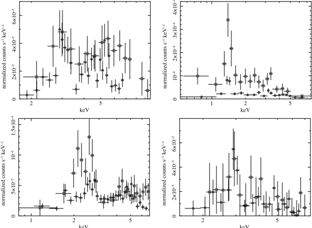
In agreement with the XMM-Newton spectral analysis, pre-sented in the previous section, four sources (PID-66, 144, 147 and 324) present FeKα lines with high (rest-frame) EW (>0.4 keV). Therefore, the joint Chandra and XMM-Newton analysis corroborates that these four sources have a good prob-ability for being Compton-thick. In Fig.1 we present the joint Chandraand XMM-Newton PN spectral fits.
5.2.2. Reflection model
We fit a reflection model,Magdziarz & Zdziarski(1995) ( + in XSPEC notation). The parameters in the PEXRAV model are the Fe abundance, the inclination angle of the reflecting slab, the cut-off energy of the incident power-law and finally the slope of the incident power-law. We found that the first three parameters remain practically unconstrained owing to the large
uncertainties. Therefore, we fix the Fe abundance to 1, and the inclination angle of to 45 degrees, while we assume that the in-cident power-law spectrum has no high energy cut-off (see e.g.
Dadina 2008).
For four sources the derived photon index is either very flat (PID-66,Γ = 0.80±0.2) or very steep (PID-222, Γ = 2.95±0.08), (PID-289,Γ = 2.90 ± 0.06), (PID-324, Γ = 2.93+0.31−0.36). As these values are many σ discrepant with the intrinsic spectral slopes encountered in AGN (see e.g.Nandra & Pounds 1994;Dadina 2008), we choose to fix the photon index toΓ = 1.8. The results are shown again in Table 2.
5.3. More complex spectral models for the four more probable Compton-thick AGN candidates
For the four more probable Compton-thick AGN candidates, we present some additional spectral models for the joint XMM-Newton and Chandra spectral fits. First, we are explor-ing the exact energy of the FeKα line. This choice is motivated by the results ofIwasawa et al.(2009) who find ionized Fe emis-sion in many Ultra-luminous IRAS galaxies. Moreover, we in-vestigate the effect of leaving the ratio between the Chandra and the XMM-Newton power-law normalization free. We keep the Fe line normalization constant, as this is believed to arise far away from the black hole in type-2 AGN (Shu et al. 2011). Therefore, the present model has two more free parameters, the line energy and the Chandra power-law normalization, which is not tied up to the XMM-Newton power-law normalization (Table3). We note that the normalization of the Chandra and XMM-Newton power-laws are consistent within the errors (see discussion in Sect. 5.2.1)
A further model contains an additional power-law whose normalization has been set to 3% of the primary power-law. The slope of this power-law has been fixed to the same value as the primary (transmitted) power-law. This component mod-els the scattered (unabsorbed) component along the line of sight which is often detected in type-2 AGN (e.g.Turner et al. 1997). In this model the energy of the FeKα line is left again as a
! " # !$%# ï " &$%# ï " '$%# ï " ()*+,-./0123)4(5626 ï %2708 ï % 708 1 2 5 0 10 ï 4 2×10 ï 4 3×10 ï 4 4×10 ï 4 normalized counts s ï 1 keV ï 1 keV ! " # $ #%!$ ! # !$ ! & !'#%!$ ! & ()*+,-./0123)4(5626 ! !2708 ! ! 708 ! " # !$%# ! " &$%# ! " '$%# ! " ()*+,-./0123)4(5626 ! %2708 ! % 708
Fig. 1. X-ray Chandra (circles) and XMM-Newton PN (squares) X-ray spectra of the Compton-thick AGN candidates PID-66, PID-144 and PID-147 and PID-324. The first and second row give the transmission and reflection dominated AGN, respectively, according to the combined Chandraand XMM-Newton spectral fits. We note the high spectral response of XMM-Newton compared to Chandra at high energies.
Table 3. Joint XMM-Newton and Chandra spectral fits to the four more probable Compton-thick sources Power-law+ FeKα line (PLCABS+GA) leaving the relative XMM-Newton and Chandra normalization and the energy of the line free.
PID NH Γ E EWX EWC c (1) (2) (3) (4) (5) (6) (7) 66 78.0+4.0−8.0 1.52+0.03−0.03 6.45+0.25−0.40 0.23+0.30−0.10 0.37+0.10−0.05 3560/3008 144 80.0+7.5−7.5 1.79+0.10−0.10 6.49+0.46−0.14 0.47+0.30−0.24 0.56+0.44−0.28 3475/3008 147 20.0+4.0−8.0 0.57+0.33−0.33 6.40−0.10+0.13 0.35+0.20−0.15 0.43+0.23−0.20 3477/3008 324 <0.45 0.76+0.12−0.14 6.38+0.95−0.95 0.69+0.63−0.42 1.15+0.69−1.00 3402/3008
Notes. The columns are: (1) XMM-Newton ID. (2) Column density (in units of 1022). (3) Photon index as derived from the PLCABS model.
(4) FeKα line energy. (5) XMM-Newton rest-frame EW of the FeKα line. (6) Chandra rest-frame EW of the FeKα line. (7) c-statistic value and degrees of freedom. Note: the model is the same as that used in Table 2 except here, the FeKα line energy is free and the Chandra and XMM-Newton power-law normalizations are not tied to each other.
free parameter. The same holds for the normalization of the Chandrapower-law which is not tied to the XMM-Newton nor-malization. The results are presented in Table 4. The spectral fits are, in general, consistent with the simple power-law plus FeKα line fits. The exception is source 66 where the photon-index becomes flatter at the expense of a lower column density. In this case, because of the flatter power-law, the EW becomes higher reaching a value of 1 keV in the case of Chandra. In good agreement with the power-law model presented in Sect. 5.2.1, the four sources (PID-66, 144, 147 and 324) present FeKα line EW higher than ∼0.4 keV corroborating their classification as probable Compton-thick candidates.
6. Co-added X-ray spectra
Although there are at least four sources with large FeKα line EW, it is possible that some of the remaining sources have large EW which fail detection owing to the limited photon statistics. In order to answer this question, we derive the co-added X-ray spectrum. The objective is to detect faint FeKα emission that cannot readily be detected in a single source (e.g.Iwasawa et al. 2012b). The data stacking is a straight sum of the rest-frame spectra of individual sources. The individual spectra are binned so that they have a 2–10 keV rest-frame energy range with 200 eV channel width. The data, after background subtraction,
Table 4. Joint XMM-Newton and Chandra spectral fits to the four more probable Compton-thick candidates, using a power-law+ FeKα line + scattered emission model (PLCABS+GA+PO), leaving the relative XMM-Newton and Chandra normalization and the central energy of the line free. PID NH Γ E EWX EWC c (1) (2) (3) (4) (5) (6) (7) 66 28.3+6.1−7.0 0.16+0.04−0.07 6.45+0.28−0.32 0.41+0.25−0.20 0.99+0.60−0.40 3551/3007 144 135+18.0−16.0 2.2+0.24−0.32 6.5−0.15+0.15 0.65+0.40−0.30 0.70+0.40−0.30 3458/3007 147 8.0+6.0−4.0 1.00+0.38−0.31 6.57+0.30−0.15 0.28+0.28−0.23 0.30+0.30−0.25 3490/3007 324 <0.42 0.72+0.13−0.16 6.39+0.08−0.08 0.51+1.49−0.25 1.22+0.90−0.70 3402/3007
Notes. The columns are: (1) XMM-Newton ID. (2) Column density (in units of 1022). (3) Photon index as derived from the PLCABS model.
(4) FeKα line energy. (5) XMM-Newton rest-frame EW of the FeKα line. (6) Chandra rest-frame EW of the FeKα line. (7) c-statistic value and degrees of freedom.
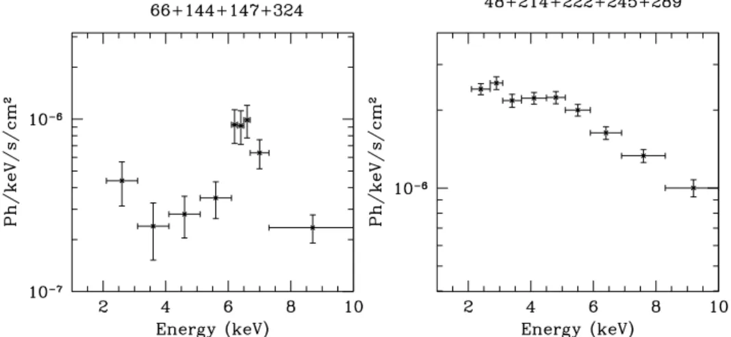
Fig. 2.Co-added (rest-frame) X-ray spectra for two sets of sources. Left panel: the four more probable Compton-thick AGN candidates (see text). Right panel: the remaining five sources.
are corrected for an efficiency curve determined by the response matrix and auxilliary response file. Finally, each energy bin is corrected for redshift.
In Fig.2, we present the co-added rest-frame X-ray spec-tra for two groups of sources. The first group includes the four more probable Compton-thick AGN candidates (PID-66, 144, 147, and 324). The second group includes the remaining sources (PID-48, 214, 222, 245, and 289). A difficulty with the second group is that two of the redshifts (PID-214 and 245) are based on the X-ray spectra and so may be more ambiguous. The first group of sources displays a very prominent FeKα line at a rest-frame energy of 6.4 keV. The second group possibly shows an emission feature but at a higher energy of about 7 keV. If con-firmed, this could imply the presence of an ionized FeKα line.
7. Infrared properties
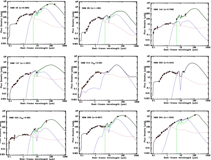
7.1. Spectral energy distributions
We construct spectral energy distributions (SED) for the full sample of our flat spectrum sources, to constrain the predom-inant powering mechanism (AGN or star formation) in the mid/far IR part of the spectrum. The SEDs are also used to obtain an accurate estimate of the 12 µm nuclear infrared luminosities and thus the X-ray to mid-IR luminosity ratios which are often considered good diagnostics for heavily obscured sources.
We use data from UV wavelengths to the far-IR (where avail-able). Four out of nine sources do not have a far-IR measure-ment available from Herschel. The data have been modelled using the code originally developed byFritz et al.(2006). The code has been updated byFeltre et al.(2012). The SED fitting is based on a multicomponent analysis (e.g.Vignali et al. 2009;
Hatziminaoglou et al. 2009;Pozzi et al. 2012). The observed UV to far-IR SED is de-composed into three distinct components: a) stars, having the bulk of the emission in the optical/near-IR b) hot dust, mainly heated by UV/optical emission caused by gas accreting onto the supermassive black hole c) colder dust heated by star formation. The stellar component has been included us-ing a set of simple stellar population (SSP) spectra of solar metallicity and ages ranging from ≈1 Myr to ≈8 Gyr. A common value of extinction is applied to stars of all ages, and aCalzetti et al.(2009) attenuation law has been adopted (RV = 4.05). To
model the emission at observed wavelengths greater than 24 µm, the SED fitting also includes a component from colder, diffuse dust, most likely heated by start formation processes, as dis-cussed below. This is represented by templates of known star-burst galaxies (Vignali et al. 2009). The SED fits are shown in Fig.3. The four more probable Compton-thick candidates ap-pear to have star-forming components. However, the strength of the star-forming component in PID-66 and PID-147 is ambigu-ous because of the lack of far-IR data in these sources. The use of templates of nearby starbursts to model the far-IR emission and hence star-formation rates, may present some limitations
Fig. 3.Spectral energy distributions of the nine possible Compton-thick candidates. The red (dot), blue (short dash), and green (long dash) lines denote the stellar, torus, and starburst component, respectively, while the black line denotes the sum of the three components.
because there may be discrepancies between typical IR SEDs at high redshift compared to local sources (e.g.Elbaz et al. 2011;
Nordon et al. 2012).
Next, we derive the exact star-formation rates and specific star-formation rates, i.e. the ratio of star-formation over the stel-lar mass. The far-IR luminosity is probably the most reliable tracer of star-forming activity (Kennicutt & Evans 2012). The IR photons are emitted by the dust surrounding young stars, which is heated by their ultra-violet radiation. The star-formation rate is derived from the total IR luminosity (8−1000 µm) which is ascribed to star-formation according to the SED decomposi-tion. We use the relation between the IR luminosity and SFR inMurphy et al.(2011):
SFR[M yr−1]= 3.88 × 10−44L(8−1000 µm)[erg s−1]. (1)
Then, the specific star-formation rate, sSFR, is given by logs SFR[Gyr−1]= log SFR[M yr−1] − log M?[M ]+ 8.77. (2)
The stellar mass M? is estimated from the optical part of the SED (for details see Rovilos et al. 2012). Table 5 sum-marises the IR luminosities, star-formation rate and stellar masses for the heavily obscured AGN in our sample. The typical errors on the 12 µm are about 20% apart from PID-48, PID-66, PID-222, and PID-245 where the uncertainties can be as high as a factor of two. In most cases, the typical errors on the total IR
luminosity are between 10 and 20%. In the cases where no far-IR data are available, the errors become large (factors of 2–3). Finally, for the stellar masses the errors are of the order of 10%.
7.2. X-ray to IR luminosity ratios
The detection of a low X-ray to mid-IR luminosity ratio has been widely used as the main instrument for the detection of faint Compton-thick AGN which cannot be easily identified in X-ray wavelengths (e.g.Goulding et al. 2011). This is because the mid-IR luminosity (e.g. 12 µm or 6 µm) is a good proxy of the AGN power, as it should be dominated by very hot dust which is heated by the AGN (e.g.Lutz et al. 2004;Maiolino et al. 2007). At these wavelengths the contribution by the stellar-light and colder dust heated by young stars should be small.Gandhi et al.(2009) present high angular resolution mid-IR (12 µm) servations of the nuclei of 42 nearby Seyfert galaxies. These ob-servations provide the least contaminated core fluxes of AGN. These authors find a tight correlation between the near-IR fluxes and the intrinsic X-ray luminosity. Although the Spitzer obser-vations do not have the spatial resolution to resolve the core, the SED decomposition allows us to derive with reasonable ac-curacy the nuclear IR luminosity. In Fig.4, we present the ob-scured X-ray luminosities against the 12 µm luminosities. All four candidate Compton-thick sources have low LX/L12 ratios.
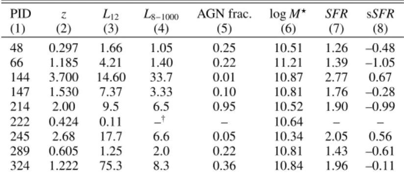
Table 5. Infrared properties of heavily obscured sources.
PID z L12 L8−1000 AGN frac. log M? SFR sSFR
(1) (2) (3) (4) (5) (6) (7) (8) 48 0.297 1.66 1.05 0.25 10.51 1.26 –0.48 66 1.185 4.21 1.40 0.22 11.21 1.39 –1.05 144 3.700 14.60 33.7 0.01 10.87 2.77 0.67 147 1.530 7.37 3.33 0.10 10.81 1.76 –0.28 214 2.00 9.5 6.5 0.95 10.52 1.90 –0.99 222 0.424 0.11 –† – 10.64 – – 245 2.68 17.7 6.6 0.05 10.34 2.05 0.56 289 0.605 1.25 2.0 0.22 10.81 1.43 –0.61 324 1.222 75.3 8.3 0.36 10.84 1.96 –0.11
Notes. The columns are: (1) XMM-ID; (2) redshift; (3) rest-frame 12 µm luminosity in units of solar luminosities (×1010); (4) total IR luminosity
in units of solar luminosities (×1011); (5) AGN fraction of the total IR luminosity; (6) logarithm of stellar mass in units of solar masses; (7)
logarithm of star-formation rate in units of solar masses/yr; (8) specific star-formation rate in units of Gyr−1.(†) no photometry above 24 µm
rest-frame wavelength.
144
66
147
324 Fig. 4.Absorbed X-ray (2–10 keV) X-ray
luminos-ity against the 12 µm luminosluminos-ity. The large circles correspond to the best candidate Compton-thick sources as suggested by the large equivalent-width FeKα lines. The typical errors are of the order of 30% and 20% for the IR and X-ray luminosity re-spectively, including the uncertainties in the model fitting. The hatched diagram represents the 1σ en-velope of the local (Gandhi et al. 2009) relation. Open circles correspond to X-ray luminosities cor-rected for absorption (see Table 1). For two sources (PID-222 and PID-324) the absorbed luminosity equals the unabsorbed luminosity. The dotted line corresponds to a factor of 30 lower X-ray luminos-ity as is typical in many Compton-thick nuclei.
mid-IR (12 µm) ratio is a reliable diagnostic for the presence of heavily obscured sources. We note that the unobscured X-ray luminosity of at least two sources lies below theGandhi et al.
(2009) relation. This may suggest that these are Compton-thick despite the absence of high-EW FeKα lines.
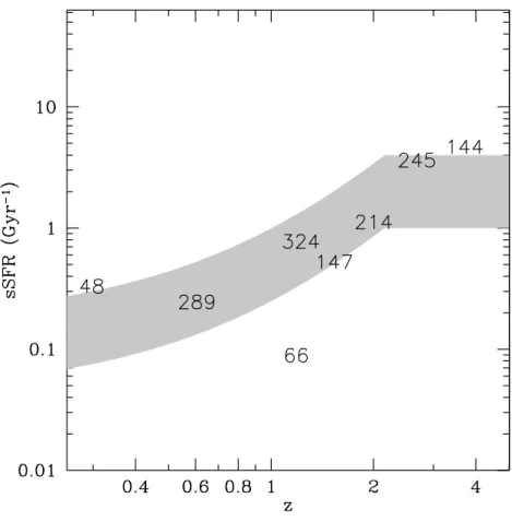
7.3. Star formation
It has been suggested that highly obscured AGN at X-ray wave-lengths may be associated with high rates of star formation (see for exampleGeorgakakis et al. 2003;Rovilos et al. 2007;
Mainieri et al. 2011). Alexander et al. (2005) find that many sub-mm galaxies, which have very high rates of star-formation, are associated with heavily absorbed sources in X-ray wave-lengths. A possible explanation for such a link would be that the nuclear star-forming region is associated with the X-ray ab-sorbing screen. In Fig.3, it appears that in the four more prob-able Compton-thick candidates, the rest-frame mid-IR wave-lengths (around 6 µm) are dominated by the torus emission.
Only two of the four probable Compton-thick candidates have long-wavelength data (PID-144, PID-324), and the star-forming component is dominated in both cases. In Fig.5 we plot the specific star-formation rate as a function of redshift. The four candidate Compton-thick sources have a specific star-formation which roughly follows the main star-forming sequence as de-scribed by Elbaz et al. (2010). Moreover, it appears that the star-formation properties of the Compton-thick AGN are not dif-ferent from those of X-ray selected AGN in general (see e.g.
Mullaney et al. 2011;Santini et al. 2012;Rosario et al. 2012;
Rovilos et al. 2012). Therefore, it appears that there is no link between the presence of a Compton-thick nucleus and enhanced star-formation activity in our sample.
8. Discussion
8.1. Limitations in the sample selection and completeness We compiled a sample of candidate Compton-thick AGN search-ing for either flat spectrum sources, i.e. those withΓ < 1.4 (at
Fig. 5.Specific star-formation rate as a function of redshift for eight of the candidate Compton-thick sources. The shaded area gives the star-formation main-sequence according to Elbaz et al. (2010). Above and below this area lie the starburst and quiescent galaxies respectively. Source 222 is not ploted as there is no available rest-frame photome-try above a rest-frame wavelength 24 µm.
the 90% confidence level) which is suggestive of a reflection dominated spectrum (e.g.George & Fabian 1991) or those show-ing an absorption turnover suggestshow-ing a rest-frame column den-sity of>1024cm−2. The deep flux limits of the present observa-tions facilitates the detection of Compton-thick sources. This is because Compton-thick AGN are difficult to detect because they are very faint in the X-rays for the same intrinsic luminosity, meaning that many Compton-thick sources at a given luminos-ity will be missed because of the effective survey flux limits.
We find nine possible sources among the 176 XMM-Newton spectra examined. Out of these, four show FeKα lines with large equivalent-widths and so these have a higher probability of be-ing Compton-thick. Our sample is by no means complete. For example, at faint fluxes there may be sources which have flat spectra, albeit with larger error bars onΓ and hence fail our se-lection criterion. Incompleteness may also be introduced by the errors in uncertain redshifts. This is important in the cases where the Compton-thick classification is based on the detection of an absorption turnover.
Next, we discuss whether there are apparently flat X-ray spectrum sources which are not genuinely reflection domi-nated Compton-thick sources. Most AGN have a steep power-law photon index with a slope of Γ ∼ 1.8 and a dispersion of σ = 0.15 (e.g. Nandra & Pounds 1994). Sources which have a significantly flatter photon-index have a high probabil-ity of being Compton-thick. However, there are flat-spectrum sources which are probably not Compton-thick. This is because there is a degeneracy between the photon-index and the col-umn density and therefore a moderate colcol-umn density or a com-plex/multiple absorber can be mistaken as a flat photon index. For example, in Table 1, we see that source PID-66 (z = 1.185) shows a photon-index of Γ = −0.37+1.2−0.6and NH = 12+45−11 cm
−2
(3015/2498) when both the photon-index and the column den-sity are left free. When the photon-index is fixed to the more realistic value ofΓ = 1.8, the implied column density becomes NH≈ 100+20−20× 1022cm−2, while the difference in the Cash
statis-tic (3018/2500) is not statistically significant. This degeneracy can be seen even in sources with large numbers of photon counts.
Corral et al.(2011) present an X-ray spectral analysis of ∼300 AGN from the XMM-Newton bright survey. There are several sources (e.g. XBSJ134656.7+580315 at a redshift of z = 0.373), at bright fluxes ( f2−10 > 10−13erg cm−2s−1) and hence with
ex-cellent photon statistics which present a flat power-law as the best-fit.Corral et al.(2011) point out that there are no iron lines with large EW detected in these sources. If the photon-index is fixed at Γ = 1.9 the resulting column density is of the order ∼1023cm−2and therefore these sources, although certainly
heav-ily obscured, are not Compton-thick.
8.2. The X-ray spectrum of Compton-thick AGN
Additional ambiguities in the selection may be introduced by uncertainties in the X-ray spectrum of Compton-thick AGN.
Brightman & Ueda(2012) perform a selection of Compton-thick sources among the Chandra sources in the 4 Ms CDF-S data us-ing their own spectral models. These take into account Compton-scattering, the geometry of the circumnuclear matter, and the scattered nuclear light. The amount of scattered light decreases with increasing column density. They find two sources with a large scattering component (>5%) and hence steeper spectra. These amounts of scattered light are well above those detected in local Compton-thick AGN (e.g.Comastri et al. 2010). Evidently, Compton-thick sources with steep spectra would have avoided detection in our selection criterion.
The strength of the FeKα line introduces an additional uncertainty. The presence of an FeKα line with a large EW is considered to be the “smoking gun” for the presence of a Compton-thick nucleus. Comastri et al.(2010) present Suzaku observations of a few Compton-thick sources. They find narrow FeKα lines (EW ∼ 1–2 keV) due to neutral or mildly ionized gas in all of them.Fukazawa et al.(2011) present Suzaku observa-tions of a sample of nearby Seyfert galaxies among which many are Compton-thick. They find that all Compton-thick sources present FeKα lines with an EW exceeding 0.5 keV. However, there have been rare examples of Compton-thick sources with small EW. One of these examples is the Broad-absorption-Line QSO Mrk231. Its BeppoSAX spectrum (Braito et al. 2004) shows that it is Compton-thick (with a column density of ∼1024cm−2), but it has an FeKα line with an EW of only 0.3 keV. Moreover, recent Suzaku observations showed a decrease in the covering fraction of the absorber (Piconcelli et al. 2013).
8.3. Previous studies of heavily obscured AGN in the CDF-S
Tozzi et al.(2006) first derived a sample of candidate Compton-thick sources in the 1 Ms CDF-S observations based on X-ray spectral fits. They derived a sample of 20 candidate Compton-thick sources. Georgantopoulos et al. (2007) per-formed the same exercise compiling a sample of 18 sources in the same dataset but using slightly different spectral mod-els. Only nine of the sources are common in these two samples, demonstrating that the uncertainties in this technique are consid-erable. From the Compton-thick candidates inTozzi et al.(2006) orGeorgantopoulos et al.(2007), only two sources are found in our present XMM-Newton sample.
Comastri et al.(2011) used the 3 Ms XMM-Newton data in the CDF-S attempting to confirm that some of the Compton-thick candidates in the above samples are most probably Compton-thick AGN. The excellent quality XMM-Newton data and in particular its ability to detect the FeKα line allowed the above authors to confirm the best two examples of Compton-thick candidates in the high redshift Universe, PID-144 and PID-147 at redshifts of z = 1.53 and z = 3.7 respectively. We note that PID-144 was first reported as Compton-thick by
Norman et al.(2002) on the basis of 1 Ms Chandra spectroscopy. For PID-144, Comastri et al. (2011) fit an absorbed power-law model finding a photon-index of Γ = 1.48+0.33−0.40 with a column density of 6+3−2 × 1023 cm−2 i.e. favouring
a transmission-dominated heavily obscured source. Moreover, they detect a strong FeKα line with an EW of 840+290−420 eV. Our joint XMM-Newton/Chandra spectral fit (Table 2) suggests a transmission-dominated highly obscured spectrum with NH ∼
5+4−3× 1023 cm−2and a photon index ofΓ = 1.26+0.72
−0.47fully
con-sistent with the results ofComastri et al.(2011). The FeKα line EW is somewhat lower (610+430−300eV) but fully consistent with the above results.
In the case of PID-147, Comastri et al. (2011) find that a good fit to the data is provided by an absorbed power-law model with a column density of 5+4−2 × 1022 cm−2 and a
pho-ton index of Γ = −0.11 ± 0.22; the iron line has a very large EW (1870+410−450 eV). Our combined XMM-Newton and Chandraspectral fits (Table 2) give a higher column density of 19+5−7× 1022cm−2but with a steeper photon-indexΓ ≈ 0.46+0.45
−0.20,
from which a smaller equivalent width (430+200−200 eV). Further exploration of the spectra suggests that the difference can be ascribed to degeneracies in the parameter space, coupled with the different treatment of statistic (c-stat vs. χ2) and binning of
the spectra, which may result in different local minima for the statistic parameter.
Brightman & Ueda (2012) report 20 Compton-thick AGN. Out of these, five have been reported as Compton-thick inTozzi et al.(2006) while three inGeorgantopoulos et al.(2007). The two Compton-thick sources reported byComastri et al.(2011) (144 and 147) and in our paper have column densities just be-low 1024cm−2in the spectral fits ofBrightman & Ueda(2012).
Recently,Iwasawa et al. (2012a) have performed a search for heavily obscured AGN in the same XMM-Newton sample as the one presented here. They are using an X-ray colour-colour dia-gram based on the rest-frame 3–5 keV, 5–9 keV, and 9–20 keV bands. They find a sample of seven candidate heavily obscured sources at high-redshift (z > 1.7) having rest-frame 9–20 keV excess emission. Some of them are good Compton-thick candi-dates either on the basis of a high-EW (>1 keV) FeKα line (e.g. PID-114 at z = 1.806) or directly on the basis of large column densities (NH≈ 1024cm−2) (PID-245, 252).
8.4. Comparison with X-ray background synthesis models We compare the number of Compton-thick AGN found here with the predictions of X-ray background synthesis models (e.g.Gilli et al. 2007; Treister et al. 2009a; Ballantyne et al. 2011; Akylas et al. 2012) In our sample, we find four prob-able candidate Compton-thick sources two of which appear to be transmission-dominated. Comparing with the models ofGilli et al.(2007)2, we find that the number of Compton-thick sources is ≈7 in our field down to the flux limit of the present sur-vey f(2−10) ∼ 1 × 10⁻¹⁵ erg cm−2s−1. The model of Treister
et al. (2009a)3 predicts a number of 8 Compton-thick in the same area. Finally, the model of Akylas et al.(2012)4 yields
about 11 Compton-thick sources in our field. All the above esti-mates refer only to transmission dominated (log NH = 24−25)
Compton-thick AGN. If we include the reflection-dominated AGN (log NH = 25−26) in the model ofGilli et al.(2007), the
total number of Compton-thick AGN rises to ≈11. Interestingly, the model of Akylas et al. (2012) has a lower intrinsic frac-tion of Compton-thick AGN compared to that of Gilli et al.
(2007), 15% compared to 33%. However, the higher number of Compton-thick AGN predicted by Akylas et al. (2012) at the relatively bright fluxes probed here, is a consequence of the stronger reflection component predicted by this model. The fact that the number of the Compton-thick candidates found here is systematically lower than those predicted by all X-ray back-ground synthesis models may suggest that our sample suffers from incompleteness.
8.5. Concluding remarks
The selection of Compton-thick AGN on the basis of either an absorption turnover (transmission dominated) or a flat spec-trum (reflection dominated) appears to be sufficiently robust. The presence of a high EW FeKα line can be considered as the fi-nal diagnostic for the presence of a Compton-thick AGN despite some possible exceptions mentioned above (e.g. Mrk 231). On the basis of the above diagnostic, we isolate four sources as ex-cellent candidates for being Compton-thick. These are probably the best Compton-thick candidates at moderate to high redshifts found so far. Still, the number found here is a factor of at least 2 www.bo.astro.it/~gilli/counts.html
3 agn.astroudec.cl 4 indra.astro.no.gr
two lower compared to the predictions of X-ray background syn-thesis models. This may imply that a number of Compton-thick AGN (particularly those at the faintest fluxes) fail to be classified as Compton-thick. It is likely that these lie among our remaining five flat spectrum sources. Then we did not classify them se-curely as Compton-thick because we failed to detect strong EW FeKα lines. The fact that a few sources lie below the Gandhi et al. (2009) unabsorbed X-ray-to-IR luminosity relation may point towards this scenario. This stresses the need for comple-mentary IR methods together with X-ray spectroscopy, to better understand the properties of Compton-thick AGN.
9. Summary
We report on an X-ray spectral study of the 176 brightest sources in the XMM-Newton survey in the CDF-S. The aim is to identify very highly obscured (Compton-thick) AGN. Our methodology consists of looking for sources which have either an absorption cut-off characteristic of a high column density or a flat spec-trum (the 90% upper limit of the photon index should be lower than 1.4). After the selection of our candidate sources, we are also looking for the presence of a strong FeKα line which is considered to be the trademark of a highly obscured source. Our results can be briefly summarised as follows:
– The XMM-Newton spectra select nine Compton-thick can-didates. We separate a group of four sources which have large iron line EW and, therefore, these have higher prob-ability of being Compton-thick. Adding the Chandra data to the spectral fits corroborates our previous results. Two of the sources are most likely transmission dominated (PID-66 and PID-144), while the other two are reflection dominated (PID-147 and PID-324).
– Although our sample is by no means statistically complete, it represents the examples of Compton-thick AGN at moderate to high redshifts. In particular, the redshifts of the four most probable candidate Compton-thick sources are z = 1.185, 1.222, 1.53 and 3.7. One of our probable Compton-thick candidates (PID-66) is presented here for the first time. The XMM-Newton spectra of two sources (PID-144 and PID-147) have been reported inComastri et al.(2011) while their combined XMM/Chandra spectrum is presented here for the first time. Finally, one source (PID-324) has been re-ported in detail inGeorgantopoulos et al. (2011a).
– The X-ray-to-mid-IR (12 µm) luminosity ratio of the four more probable Compton-thick candidates are well below the average relation ofGandhi et al.(2009), independently sug-gesting heavy obscuration.
– Spitzer and Herschel observations of our four candidate Compton-thick sources derive star-formation rates between about 25 and 1000 M yr−1. Their specific star-formation
rates are consistent with those of normal galaxies sug-gesting that heavy obscuration is not related to enhanced star-formation.
Acknowledgements. I.G. and A.C. acknowledge the Marie Curie fellowship
FP7-PEOPLE-IEF-2008 Prop. 235285. We acknowledge financial contribution from the agreement ASI-INAF I/009/10/0. P.R. acknowledges the receipt of a fellowship (proposal no. P9-3493) from the Greek Secretariat of Research and Technology in the framework of the project “Support to postdoctoral re-searchers”. N.C. acknowledges financial support from the Della Riccia founda-tion. F.J.C. acknowledges partial financial support by the Spanish Ministry of Economy and Competitiveness through the grant AYA2010-21490-C02-01. The
Chandradata used were taken from the Chandra Data Archive at the Chandra
X-ray Center.
References
Ajello, M., Rau, A., Greiner, J., et al. 2008, ApJ, 673, 96 Akylas, A., & Georgantopoulos, I. 2009, A&A, 500, 999
Akylas, A., Georgakakis, A., Georgantopoulos, I., Brightman, M., & Nandra, K., 2012, A&A, 546, A98
Alexander, D. M., Bauer, F. E., Brandt, W. N., et al. 2003, AJ, 126, 539 Alexander, D. M., Bauer, F. E., Chapman, S. C., et al. 2005, ApJ, 632, 736 Alexander, D. M., Chary, R. R., Pope, A., et al. 2008, ApJ, 687, 835 Alexander, D. M., Bauer, F. E., Brandt, W. N., et al. 2011, ApJ, 738, 44 Arnaud, K. A. 1996, Astronomical Data Analysis Software and Systems V,
eds. G. Jacoby, & J. Barnes, ASP Conf. Ser., 101, 17 Balestra, I., Mainieri, V., Popesso, P., et al. 2010, A&A, 512, A12
Ballantyne, D. R., Draper, A. R., Madsen, K. K., Rigby, J. R., & Treister, E., 2011, ApJ, 736, 56
Barger, A., Cowie, L., Capak, P., et al. 2003, AJ, 126, 632 Braito, V., Della Ceca, R., Piconcelli, E., et al. 2004, A&A, 420, 79 Brandt, W. N., & Hasinger, G. 2005, ARA&A, 43, 827
Brightman, M., & Nandra, K. 2011, MNRAS, 413, 1206 Brightman, M., & Ueda, Y. 2012, MNRAS, 423, 702 Burlon, D., Ajello, M., Greiner, J., et al. 2011, ApJ, 728, 58 Calzetti, D. 2009, ASPC, 414, 214
Cardamone, C. N., van Dokkum, P. G., Urry, C. M., et al. 2010, ApJS, 189, 270 Cash, W. 1979, ApJ, 228, 939
Churazov, E., Sunyaev, R., Revnivtsev, M., et al. 2007, A&A, 467, 529 Comastri, A. 2004, ASSL, 308, 245
Comastri, A., Iwasawa, K., Gilli, R., et al. 2010, ApJ, 717, 787 Comastri, A., Ranalli, P., Iwasawa, K., et al. 2011, A&A, 526, L9 Cooper, M. C., Yan, R., Dickinson, M., et al. 2012, MNRAS, 425, 2116 Corral, A., Della Ceca, R., Caccianiga, A., et al. 2011, A&A, 530, A42 Daddi, E., Alexander, D. M., Dickinson, M., et al. 2007, ApJ, 670, 173 Dadina, M. 2008, A&A, 485, 417
Dahlen, T., Mobasher, B., Dickinson, M., et al. 2010, ApJ, 724, 425 Damen, M., Labbé, I., van Dokkum, P. G., et al. 2011, ApJ, 727, 1 Dickey, J. M., & Lockman, F. J. 1990, ARA&A, 28, 215
Eckart, M. E., McGreer, I. D., Stern, D., Harrison, F. A., & Helfand, D. J. 2010, ApJ, 708, 584
Elbaz, D., Hwang, H. S., Magnelli, B., et al. 2010, A&A, 518, L29 Elbaz, D., Dickinson, M., Hwang, H. S., et al. 2011, A&A, 533, A119 Feltre, A., Hatziminaoglou, E., Fritz, J., & Franceschini 2012, MNRAS, 426,
120
Feruglio, C., Daddi, E., Fiore, F., et al. 2011, ApJ, 729, L4 Fiore, F., Grazian, A., Santini, P., et al. 2008, ApJ, 672, 94 Fiore, F., Puccetti, S., Brusa, M., et al. 2009, ApJ, 693, 447
Fritz, J., Franceschini, A., & Hatziminaoglou, E. 2006, MNRAS, 366, 767 Frontera, F., Orlandini, M., & Landi, R. 2007, ApJ, 666, 86
Fukazawa, Y., Hiragi, K., Mizuno, M., et al. 2011, ApJ, 727, 19 Gandhi, P., Horst, H., Smette, A., et al. 2009, A&A, 502, 457
Georgakakis, A., Hopkins, A. M., Sullivan, M., et al. 2003, MNRAS, 345, 939
Georgantopoulos, I. 2012 [arXiv:1204.2173]
Georgantopoulos, I., Georgakakis, A., & Akylas, A. 2007, A&A, 466, 823 Georgantopoulos, I., Georgakakis, A., Rowan-Robinson, M., & Rovilos, E.
2008, A&A, 484, 671
Georgantopoulos, I., Akylas, A., Georgakakis, A., & Rowan-Robinson, M. 2009, A&A, 507, 747
Georgantopoulos, I., Dasyra, K., Rovilos, E., et al. 2011a, A&A, 531, A116 Georgantopoulos, I., Rovilos, E., Xilouris, E. M., Comastri, A., & Akylas, A.
2011b, A&A, 526, A86
George, I., & Fabian, A. C. 1991, MNRAS, 249, 352
Giacconi, R., Gursky, H., Paolini, F. R., & Rossi, B. B. 1962, Phys. Rev. Lett., 9, 439
Giacconi, R., Zirm, A., Wang, J., et al. 2002, ApJS, 139, 369 Gilli, R., Comastri, A., & Hasinger, G. 2007, A&A, 463, 79 Gilli, R., Vignali, C., Mignoli, M., et al. 2010, A&A, 519, A92 Gilli, R., Su, J., Norman, C., et al. 2011, ApJ, 730, L28
Goulding, A. D., Alexander, D. M., Mullaney, J. R., et al. 2011, MNRAS, 411, 1231
Goulding, A. D., Alexander, D. M., Bauer, F. E., et al. 2012, ApJ, 755, 5 Hatziminaoglou, E., Fritz, J., & Jarrett, T. H. 2009, MNRAS, 399, 1206 Iwasawa, K., Crawford, C. S., Fabian, A. C., & Wilman, R. J. 2005, MNRAS,
326, L20
Iwasawa, K., Sanders, D. B., Evans, A. S., et al. 2009, ApJ, 695, L103 Iwasawa, K., Gilli, R., Vignali, C., et al. 2012a, A&A, 546, A84 Iwasawa, K., Mainieri, V., Brusa, M., et al. 2012b, A&A, 537, A86 Kennicutt, R. C., & Evans, N.J., 2012, ARA&A, 50, 531 Le Fèvre, O., Vettolani, G., Garilli, B., et al. 2005, A&A, 439, 845 Lehmer, B. D., Brandt, W. N., Alexander, D. M., et al. 2005, ApJS, 161, 21 Luo, B., Bauer, F. E., Brandt, W. N., et al. 2008, ApJS, 179, 19
Luo, B., Brandt, W. N., Xue, Y. Q., et al. 2010, ApJS, 187, 560
Lutz, D., Maiolino, R., Spoon, H. W. W., & Moorwood, A. F. M. 2004, A&A, 418, 465
Magdziarz, P. A., & Zdziarski, A. 1995, MNRAS, 273, 837 Magnelli, B., Elbaz, D., Chary, R. R., et al. 2009, A&A, 496, 57 Mainieri, V., Bongiorno, A., Merloni, A., et al. 2011, A&A, 535, A80 Maiolino, R., Shemmer, O., Imanishi, M., et al. 2007, A&A, 468, 979 Malizia, A., Bassani, L., Bazzano, A., et al. 2012, MNRAS, 426, 1750 Marconi, A., Risaliti, G., Gilli, R., et al. 2004, MNRAS, 351, 169 Matt, G., Bianchi, S., Guainazzi, M., & Molendi, S. 2004, A&A, 414, 155 Merloni, A., & Heinz, S. 2008, MNRAS, 388, 1011
Moretti, A., Pagani, C., Cusumano, G., et al. 2009, A&A, 493, 501 Moretti, A., Vattakunnel, S., Tozzi, P., et al. 2012, A&A, 548, A87
Mullaney, J. R., Alexander, D. M., Goulding, A. D.. & Hickox, R. C. 2011, MNRAS, 414, 1082
Murphy, E. J., Condon, J. J., & Schinnerer, E. 2011, ApJ, 737, 67 Nandra, K. & Pounds, K. A., 1994, MNRAS, 268, 405 Nordon, R., Lutz, D., Genzel, R., et al. 2012, A&A, 745, A182 Norman, C., Hasinger, G., Giacconi, R., et al. 2002, ApJ, 571, 218 Norris, R. P., Afonso, J., Appleton, P. N., et al. 2006, AJ, 132, 2409 Oliver, S., Bock, J., Altieri, B., et al. 2012, MNRAS, 424, 1614 Paltani, S., Walter, R., McHardy, I. M., et al. 2008, A&A, 485, 707 Piconcelli, E., Miniutti, G., Ranalli, P., et al. 2013, MNRAS, 428, 1185 Pozzi, F., Vignali, C., Gruppioni, C., et al. 2012, MNRAS, 423, 1909 Rafferty, D. A., Brandt, W. N., Alexander, D. M., et al. 2011, ApJ, 742, 3 Ranalli, P., Comastri, A., Vignali, C., et al. 2013, A&A, 555, A42 Ravikumar, C. D., Puech, M., Flores, H., et al. 2007, A&A, 465, 1099 Ricci, C., Walter, R., Courvoisier, T. J.-L., & Paltani, S. 2011, A&A, 532, A102
Rosario, D. J., Santini, P., Lutz, D., et al. 2012, A&A, 545, A45
Rovilos, E., Georgakakis, A., Georgantopoulos, I., et al. 2007, A&A, 466, 119
Rovilos, E., Comastri, A., Gilli, R., et al. 2012, A&A, 546, A58 Santini, P., Fontana, A., Grazian, A., et al. 2009, A&A, 504, 751 Santini, P., Rosario, D. J., Shao, L., et al. 2012, A&A, 540, A109
Sazonov, S., Krivonos, R., Revnivtsev, M., Churazov, E., & Sunyaev, R. 2008, A&A, 482, 517
Silverman, J. D., Mainieri, V., Salvato, M., et al. 2010, ApJS, 191, 124 Shu, X. W., Yaqoob, T., & Wang, J. X. 2011, ApJ, 738, 147
Soltan, A. 1982, MNRAS, 200, 115
Szokoly, G. P., Bergeron, J., Hasinger, G., et al. 2004, ApJS, 155, 271 Taylor, E. N., Franx, M., van Dokkum, P. G., et al. 2009, ApJS, 183, 295 Tozzi, P., Gilli, R., Mainieri, V., et al. 2006, A&A, 451, 457
Treister, E., Urry, C. M., & Virani, S. 2009a, ApJ, 696, 110
Treister, E., Cardamone, C. N., Schawinski, K., et al. 2009b, ApJ, 706, 535 Tueller, J., Mushotzky, R. F., Barthelmy, S., et al. 2008, ApJ, 681, 113 Turner, J. T., George, I. M., Nandra, K., & Mushotzky, R. F. 1997, ApJ, 488, 164 Vanzella, E., Cristiani, S., Dickinson, M., et al. 2008, A&A, 478, 83
Vignali, C., Pozzi, F., Fritz, J., et al. 2009, A&A, 395, 2189
Winter, L. M., Mushotzky, R. F., Reynolds, C. S., & Tueller, J. 2009, ApJ, 690, 1322
Worsley, M. A., Fabian, A. C., Bauer, F. E., et al. 2005, MNRAS, 357, 1281 Worsley, M. A., Fabian, A. C. Pooley, G. G., & Chandler, C. J. 2006, MNRAS,
368, 844
Xue, Y. Q., Luo, B., Brandt, W. N., et al. 2011, ApJS, 195, 10 Xue, Y. Q., Wang, S. X., Brandt, W. N., et al. 2012, ApJ, 758, 129 Yaqoob, T. 1997, ApJ, 479, 184