Creation of tools for manipulation tasks through Task and motion Planning using differentiable physics

Creation of Tools for Manipulation Tasks through

Task and Motion Planning using Differentiable Physics

by

Christina Wettersten

Submitted to the Department of Electrical Engineering and Computer

Science

in partial fulfillment of the requirements for the degree of

Master of Engineering in Computer Science and Electrical Engineering

at the

MASSACHUSETTS INSTITUTE OF TECHNOLOGY

June 2019

© Massachusetts Institute of Technology 2019. All rights reserved.

Author ………

Department of Electrical Engineering and Computer Science

May 16, 2019

Certified by ………

Tomás Lozano-Pérez

Professor

Thesis Supervisor

Accepted by ……….

Katrina LaCurtis

Chair, Master of Engineering Thesis Committee

Creation of Tools for Manipulation Tasks through Task and Motion Planning

using Differentiable Physics

by Christina Wettersten

Submitted to the Department of Electrical Engineering and Computer Science May 16, 2019


In Partial Fulfillment of the Requirements for the Degree of Master of Engineering in Electrical Engineering and Computer Science

Abstract

Toussaint et al. [1] have proposed a novel embedding of dynamic physical

manipulations within a Task And Motion Planning (TAMP) framework to achieve a subset of sequential manipulation tasks involving tools. The work, in part, mimics the human ability to plan using an ‘intuitive physics engine’ [2] by using physics-based primitives in task planning. The primitives are described by the stable kinematic or differentiable dynamic and impulse exchange constraints they impose on the robot during motion planning. By altering and expanding the set of primitives, to include modification and recombination of items in the work space, I present an expansion upon this approach using to achieve not only tool use, but tool creation. The new approach is then tested on three classes of problems: rerunning previous tool use problems, problems designed to recreate previously seen tools and manipulation problems in workspaces with significant obstacles.

Acknowledgements

I have had the great fortune to be supported by many people. I would like to thank my advisor Professor Tomás Lozano-Pérez for giving me both invaluable critique and strong encouragement to keep trying. I would like to thank Marc Toussaint for the inspiration for this thesis work. Finally I would like to thank my friends for keeping me sane and my family for making all this possible.

Contents

Chapter 1: Introduction………..7

Chapter 2: Related Work……….11

2.1 Motion Planning………12

2.2 Multi-Modal Motion Planning………14

2.3 Trajectory Optimization………..15

2.4 Multi-Modal Optimization………..17

2.5 Task And Motion Planning (TAMP)………..18

Chapter 3: Logic-Geometric Program (LGP)……….21

3.1 General Problem Formulation………..21

3.2 Logic Geometric Problem Formulation……….23

3.3 Modes and Actions……….25

3.4 Basic Predicates and Problem Definition……….27

3.5 Solving a Logic Geometric Program………..28

Chapter 4: Tool Creation Problems in a Logic-Geometric Program

(LGP)……….30

4.1 Added Geometric Predicates………31

4.2 Added Action Operators……….32

4.3 Logical Predicates and Object Labels………33

4.4 Building Blocks and Attach 2.0……….34

4.5 World and Problem Definition………...35

Chapter 5: Experiments, Results and Future Work………..37

5.1 Rerunning Tool Use Problems………..38

5.2 Recreating Tools from Tool Use Problems………....41

5.3 Creating New Tools in Obstacle Problems………....48

5.4 General Findings and Conclusions………..54

5.5 Future Work………56

References………..58

List of Figures

Fig 4.1.1 Example of Starting Conditions………31

Fig 4.4.1 Illustration of Attachable Regions on Building Blocks…..35

Fig 5.1.1 Example of a Simple Tool Use Plan……….38

Fig 5.1.2 Example of a Plan Without New Actions….………...39

Fig 5.1.3 Example of a Plan With New Actions………..39

Fig 5.1.4 Example of a Plan Involving Throwing……….40

Fig 5.1.5 Plot Comparing Solution Times With New Actions……...40

Fig 5.1.6 Illustration of Different Attach Constraints………..41

Fig 5.2.1 Example of Normal Hook Problem………42

Fig 5.2.2 Example of a Plan With a Broken Hook………42

Fig 5.2.3 Plans Produced With Hook Pieces Starting Scattered…..43

Fig 5.2.4 Plot Comparing Solution Times For Different Starting

Placements………44

Fig 5.2.5 Plan With Two Pieces Shifted Left………44

Fig 5.2.6 Plan With Pieces Vertically Aligned………..45

Fig 5.2.7 Plot Comparing Solution Times For Different Starting

Orientations………...45

Fig 5.2.8 Plan With Pieces Rotated Horizontally……….46

Fig 5.2.9 Plot Comparing Solution Times For Different Piece

Lengths………..46

Fig 5.2.10 Examples of Problems Involving Hitting………47

Fig 5.3.1 Plan With a Break and Attach………48

Fig 5.3.2 Plans With Target Object Under an Obstacle……….……49

Fig 5.3.3 Plans With Target Object On a Tall Obstacle………..50

Fig 5.3.4 Illustrations of Plans with Collisions……….51

Fig 5.3.5 Examples of Collisions with Added Obstacles…………...52

Fig 5.3.6 Examples of Plans Throwing through Obstacles…………52

Fig 5.3.7 Plot Comparing Solution Times With and Without

Obstacles ………..53

Fig 5.4.1 Plot Comparing All Solution Times………55

1 Introduction

A raven drops a nut onto the crosswalk of a busy intersection to safely crush it, and becomes the star of a viral video on smartest birds [3]. Dolphins are observed to use sponges as armor and papers are written about their comparatively vast

intelligence [4]. When we see animals using items in their environment as tools to solve tasks, we acknowledge they have a certain level of intelligence [5], because using tools requires a certain capability for prediction of outcomes on possible actions and

creativity of thought to propose various solutions.

When trying to replicate similar results with robots, researchers and

programmers face a seemingly insurmountable task. To search for and find the motor inputs required to simply grasp an object is already complex. Now imagine trying to search for the motor inputs required to complete a whole maneuver of grasping, picking up and moving various items. As the length of the full solution increases, the number of possible motor inputs to search over grows exponentially.

Finding a way to structure this search and reduce the number of potential solutions considered is imperative. Task and Motion Planning (TAMP) partially separates out the low level control optimization providing specific motor inputs (trajectory optimization) from the logical search over a sequence of possible actions (task planning). By guiding the search to only consider possibly useful actions, e.g. grasping an object, the number of solutions to search through is reduced significantly. Due to their increased efficiency, approaches with Task and Motion Planning have shown success in domains with complicated and lengthly plans that plain motion planners struggle to find solutions for.

But these solutions are typically still limited to specifically defined prehensile actions the researchers carefully craft for the robot. Additionally, they generally produce less than optimal solutions as they break sections of each plan into problems to solve independently. They lack the full creativity found in human and animal tool creation and problem solving. Research in cognitive science shows that humans may be particularly good at solving sequential manipulation tasks like these due to an ‘intuitive physics engine’ [2] which allows us to simulate the outcome of our possible actions.

Toussaint et al. proposed incorporating the constraints of the physical

interactions between objects as part of the search in task planning as opposed to only specific predefined actions, giving robots a similar way to search with their own

‘physics engine’. The system proposed in [1] approached manipulation tasks in the shape of Logic Geometric Programs, a way to formalize the relationship between the logical sequence of actions and the physical interactions and geometric constraints they impose. This allowed the system to solve the whole long problem as one optimization problem instead of arbitrarily breaking it down into subsections.

By optimizing the whole path at once, requirements on the grasp pose for a final step could be set up correctly on the first grasp. The solutions found by a Branch and Bound solver proposed in [1] on the LGPs showed near optimal solutions on tasks using simple tools. This thesis is about expanding that work to allow for solutions that not only use tools, but create them.

To show not only tool use, but tool creation, two new actions were defined. In addition to possible actions like hit or throw the new actions attach and break were added. Additional logical concepts to facilitate the new actions (‘attached’,

‘attachable’) were also added. This allowed the solver to correctly reason about when the new actions could be used.

The actions were first tested on the previous experiments[1] to see how the added actions changed the solver’s efficiency. The next set of experiments closely mirrored the previous experiments, but were designed to see if the system would recreate tools similar to those it had been shown to successfully use. The final set of experiments were new problems designed to stretch the solver’s capabilities and explore the limits of the system with the new actions.

The system preformed nearly the same on the set of previous tool use problems, as expected. Since the logical state for the new actions were rarely applicable and generally would result in more complex solutions, the solver found very similar solutions.

In problems that were similar to previous tool use problems, but started with the tools malformed or broken, the system showed creative results with a mix of solutions using the actions to create tools and solutions exploiting the simulator’s assumption of perfect physics by throwing or sliding pieces precisely to achieve the desired result. These types of solutions were are also present in the previous paper, but due to the added complexity of the solutions involving attaching or breaking, solutions with throwing or hitting were more common in these experiments.

The final set of experiments showed mixed results. Like the tool creation

problems there was a mix of tool creation and opting to simply throw a piece. In these problems with significant obstacles in the workspace, the system also showed a surprising predilection to move through obstacles despite incurring high obstacle

costs. As the goal for this thesis work was to see the capabilities of the system with a minimal amount of changes, there was not a chance to go in and significantly alter the cost computation for obstacles, however this area would be an interesting place to explore in the future.

The human and animal ability to create tools remains a difficult and interesting challenge to recreate in robotic planning and this thesis shows a brief glimpse into both what is already possible as well as what challenges are still left to face. In the following chapter a brief history of the field of Task and Motion Planning is outlined. In chapter three a more detailed explanation of the previous work done by Toussaint et al.[1] is given. A full description of the alterations and additions to the LGP system can be found in chapter four. Finally, experiment descriptions, results and areas for future work are in chapter five.

2 Related Work

Robotic task and motion planning has a long history, and the area is rich with previous approaches. For the purpose of this paper we lay out the space of related work in two major categories: planners that only consider kinematic constraints and planners that consider the dynamic feasibility of paths. Kinematic planners only consider the geometric constraints on a path- where an obstacle is, joint limits of an actuator, etc. without considering the forces that cause the motion. Planners that account for the dynamic feasibility of a path consider both the geometric constraints and the forces involved.

Problems in manipulation planning generally are described in terms of the operators or actors, for example a robot, the workspace they operate in, like a workbench, and objects to be manipulated in the world. Together the location of objects, and occasionally some added semantic information, for example discrete states based on geometric relationships (like ‘in’, ‘held’ or ‘on’), make up the state of the world. The representation of locations can be either in terms of Cartesian

coordinate space or in terms of the joint space of the robot.

A manipulation problem is typically defined with a specific starting state and a set of goal conditions which partially define a goal state. A goal condition of a specific manipulation problem could include a specific location or orientation for a particular object or a geometric relationship to something else in the workspace, e.g. block A is ‘on’ block B. The union of all the goal conditions define the set of goal states which a manipulation planner will attempt to reach. The ideal output of a planner will be a continuous motion for the robot that avoids obstacles as it reaches the goal state.

2.1 Motion Planning

For a robot to interact with the world and complete any task, it needs to move. Motion planners take in a desired movement task, such as move to the door or grasp the handle, and produces a plan of discrete motions (move a few feet forward, rotate the wrist 30 degrees clockwise) to accomplish the task.

For robotic problems in low dimensional spaces (consider a point robot on a plane with static obstacles) paths can be found by using standard search algorithms on a grid laid over the world. The robot is allowed to move between adjacent cells on a grid if the path between the two cells is fully in the robot’s free space- that is it doesn’t cause the robot to contort in ways that are infeasible or cause it to collide with an obstacle. By discretizing the space, algorithms like A* or Dijkstra can then be used to search through the possible actions.

All of these planners however are susceptible to missing paths through narrow free areas if the grid resolution is set too high, and are inefficient when the grid resolution is small. These approaches are poor choices for high dimension problems as the number of grid cells increases exponentially with the dimension of the configuration space.

A way to get away from searching through a large number of cells in a high dimension problem space is to use sample-based methods. These methods are well suited for high dimension problems as the search is no longer explicitly dependent on the dimension of the configuration space. Probabilistic Roadmaps (PRMs)[16] use sampling to first build up a graph to search over in place of a grid. The nodes sampled are connected to some k nearest nodes so long as the connection does not move

through an obstacle. Once the graph is dense enough, a standard search algorithm is applied to find a path between the start and goal.

Similar to this, RRT [17] builds a tree of collision free path segments from a start node towards new configurations sampled uniformly from the configuration space. Periodically the goal is ‘sampled’ to see if a connection is feasible to a node on the tree. Once the goal is connected, the path from the start to goal is returned. There have been many, many variants on RRT to increase efficiency and to produce more optimal results. While, sample based approaches are only probabilistically complete- they can’t definitively prove a path is infeasible and are not guaranteed to return a path if one exists, in practice these approaches have had great success.[15]

Early work in applying algorithmic motion planners to manipulation includes the Handey system [18] which looked at simple pick and place problems. Other early attempts such as by Wilfong [19] planned with a single moveable object in a world of polygon obstacles. Much of the modern work in manipulation however, is built off of a notion of multi-modal motion planning.

2.2 Multi-Modal Motion Planning

Motion planners generally consider the robot’s free space to be unchanging, however certain problems (eg manipulation, legged locomotion) are better modeled as a network of modes where each mode has constant kinematics. For example consider a manipulation task with a block. As the robot grasps the block differently, the possible valid configurations for the robot change to reflect the different ways the block grasped by the robot would come into collision with obstacles.

Alami et. al [20, 21] first introduced a ‘manipulation graph’ which breaks a single moveable object manipulation problem into subproblems to move while holding the object between connected configuration subspaces where the object can be placed and then regrasped. The solution is a sequence of motions (paths) where the robot is alternating grasping the object (transfer path) and moving without it (transit path). Building off of this, Simeon et. al. [22] used PRMs to produce more realistic and executable plans for manipulation problems involving a single moveable object. The ‘manipulation graph’ was used as a way to search for a series of grasps which then was solved using a motion planner.

To avoid trying to define this complicated space all at once Hauser and Latombe [23] proposed a generalized way to plan considering multiple modes with transitions between them. Similar to the manipulation graph, the manipulation problem can be broken down into ‘modes’ defined by differently constrained configuration spaces as dictated by grasping or the specific placement of an object. A plan can then be seen as an alternating sequence of moving in a specific mode (moving holding one object) and switching to another mode (picking up a new object, or placing an already held object). Moving through a single configuration space can be solved using existing motion planners and samples of configurations where transfers between modes can occur. As the transfer between modes is highly task dependent, a sampler would need to be constructed for any specific manipulation problem.

To address the issue of sampling perhaps rare occurrences of configurations where transitions between successive transfer and transit trajectories could occur, Barry et. al. [36] proposed DARRT which applies a RRT like search over partially

defined configurations. The RRT tree is grown by sampling subsets of configurations involving only the robot or only the target object and planning ignoring obstacles towards the new configuration. DARRT showed success in planning for manipulation problems with a single object using actions like pick, place and push.

2.3 Trajectory Optimization

All of the approaches discussed so far only consider the kinematic constraints on a robot’s path. However to move with high speeds and interact more fully with the environment, robotic manipulators particularly need to consider the dynamic feasibility of their path. Optimization based motion planners look at a manipulation problem as an optimization problem- generally starting with an imperfect guess of a motion plan that is then optimized to adhere to desired goals and constraints (like obstacle avoidance). Optimization methods use the notion of a finite number of ‘knot points’ at which a robot’s velocity and position are the decision variables for the optimization problem. The cost and objective functions are defined to reflect the constraints imposed by the dynamics of the system as well as to encode any desired behavior like robustness of the trajectory optimization or minimization of energy expended. The optimization is then solved using numerical procedures. [24]

Ratliff et al. [25] introduced a Covariant Hamiltonian Optimization for Motion Planning (CHOMP) that could take initial guesses that weren’t feasible (ie a straight line solution through obstacles) and encode the desired obstacle avoidance into the

optimization cost. This eliminated the need to find a base collision free path to then optimize, but did not guarantee the final path would be collision free.

TrajOpt [35] is related to CHOMP, with a few significant differences. The distance function is computed using the convex meshes of the objects instead of sphere

approximations getting more natural collision avoidance. TrajOpt also replaces the small gradient descent steps which modify the trajectory in CHOMP with solving a locally simplified approximation of the problem. While both of these changes are more computationally complex, due to the more faithful, and flexible representation of the real world, TrajOpt results in more realistic and executable trajectories on a wider range of problems.

2.4 Multi-Modal Optimization

As optimization looks to make cost and goal functions reasonably smooth in order to find gradients, without modification this blends poorly with manipulation problems involving contact with surfaces or objects that create discontinuities due to friction or impact. To optimize despite the discontinuities, the problem is often

constrained to a single set sequence of contacts. By knowing the sequence of when the discontinuities will occur, the optimization can be computed around them.

Hybrid optimization introduces an idea of modes and mode schedules where a sequences of modes are defined using an outer loop search and then a specific sequence can be optimized using existing methods. The notion of a hybrid mode is defined to be the set of surfaces that are actively in contact, or ‘contacts’, with the robot and factor into the kinematics or dynamics of motion. Discontinuities in the trajectory are only allowed at certain points where guard conditions are met and the

hybrid mode changes. This allows existing optimization techniques to be applied to sections of the path contained within a single hybrid mode.

For problems like walking, the structure and order of the contacts are well known and can be explicitly described [14]. The problems can be formulated as Mixed-Integer Programs (MIP) that can be solved with standard branch-and-bound

optimizers. However not all problems are as well understood. To search for a search for the sequence of modes, outer optimization loops[26] and combinatorial planners [27] have been used. Simply using Dynamic Programming to brute force the sequence has also been attempted [28] but these attempts are limited to low dimensional problems. In addition to the hybrid approach, research in mode invariant optimization methods have been explored. In problems involving only a small number of contacts, a nonlinear programing method with penalties has been used to jointly optimize for trajectories and contacts.[29] Tassa and Todorov [30] introduced using Differential Dynamic Programming (DDP) by making small gradient-inspired improvements to an initial trajectory.

Contact Invariant Optimization (CIO) [8] relaxes the contact structure to search over possible combinations of surfaces to create phases and the possible phases to create full movements. The approach allows for the complemenarity constraints that describe how outside contacts act on the robot to be expressed as costs instead of hard constraints. This allows surfaces to exert forces at a distance, but also smooths the optimization and provides more useable gradient information. While this can result in infeasible paths, it has been used successfully to preform complex robot movements like moving from sitting to standing or crawling.

Inspired by issues with hybrid control, Posa et al. [31] propose a non-linear program that avoids using discrete decision variables. Instead terms similar to those found in the linear complementary problem (LCP) are used.

All of these methods have not yet been shown to achieve higher level task planning.

2.5 Task And Motion Planning (TAMP)

By adding a task planning layer to the system, the task planner can account for logically viable solutions for problems that require specifically ordered steps, while the motion planner ensures the final solution is still executable on the robot. For problems in sequential manipulation, like tool use or tool creation, this generally means the task planner deals with the order of actions, manipulations and modes, while the motion planner secondarily attempts to generate paths as guided by the task planner. The task planner then has a great deal of control over the variance of possible solutions, and any limits imposed on how the task planner generates plans, will

necessarily be present in the solution. One of the earliest systems, Asymov [32] uses a symbolic search (in tasks) as a heuristic for the geometric search (in motion). In this system the task search ignored geometry and therefore had only limited use as a heuristic.

The typical way to represent actions in sequential manipulation for a task planner in is to describe the necessary preconditions and resulting effects [7]. For the action “grasp” for example, the preconditions could be that the robot hand is empty and the cup is on the table, and effects would be that the cup is in the hand and the hand is full.

The struggle is efficiently combining the task planner with input from the motion planner, which can find certain paths or states infeasible. Continuing our “grasp” example, say the cup on the table was blocked by another item and couldn’t be reached by the robot. The task planner then needs to either incorporate this feedback to refine its search, or a priori include a precondition for some measure of assurance that the robot can reach the cup.

Some previous work generally involves breaking the continuous robot space into discrete sections so that it can be reformulated as a Constraint Satisfaction Problem (CSP) [7, 9] or using a search over sequences formed by the task planner, paired with a standard sample based path planner proving individual actions improbable [10, 11]. Other recent work in TAMP includes FFROB [33] and later STRIPStream [34] which are similar to a PRM in that they sample the space and then try to search over the samples to find a feasible plan. Unlike PRM, the samples aren’t assembled into a graph, but are instead fed into a Planning Domain Definition Language (PDDL) task planner that searches over instances of an action (an action with a specific sampled configuration) to see if a plan can be found. The advantage of these methods is the opportunity to use existing highly efficient task planners to piece together actions defined via task-specific, custom continuous-variable samplers. While the plans

generated are non optimal, the flexibility of the method to apply across many domains is notable.

The main body of work from which this thesis is inspired uses the notions of CIO and invertible, differentiable physics (as need for optimization) in conjunction with TAMP systems. The novel Logic-Geometric Program system developed by Toussaint

et. al. [1] most closely resembles the Mixed Integer Programming (MIP) formulation of a manipulation problem, but replaces the integers (representing the set of contacts) with discrete first order logic. This allows for the set of contacts, as described by the logical state, to be guided based on a task level search (like those found in TAMP systems) instead of exhaustively searched over or optimized. Further details of the system follow in chapter 3.

3 Logic-Geometric Program (LGP)

The basis for the work in this thesis is the previous work done by Toussaint et al. [1] which showed a new approach to Task and Motion Planning (TAMP) using

optimization techniques and dynamic based flexibility found in Constraint Invariant Optimization (CIO). The new approach laid out a way to describe sequences of manipulations and actions as a Logic Geometric Program (LGP).

The LGP unlike previous approaches in TAMP explicitly defines a way to format manipulation problems using the physical static, dynamic and geometric constraints imposed by a logical sequence of actions into a single path optimization. The approach uses a notion of modes, similar to CIO, where the equations of motion describing the objects are constant. Then as with other TAMP approaches a more structured solver can guide the search over different sequences of actions to optimize only the logically reasonable sequences of actions.

3.1 General Problem Formulation

The approach laid out by Toussaint [1] involves optimizing possible paths and sequences of actions, or skeletons, as guided by logical constraints. Most generally, the overall manipulation problem is to optimally find a path from the initial configuration to the final goal state and configuration while obeying the constraints imposed by physics and limits of the robot.

In [1] the problem is formally stated as follows: Given the configuration space with a n-dimensional robot and m rigid objects with initial

configuration . The aim is to find a path

s.t.

(1)

The path constraints are in terms of the robots position, velocity and

acceleration which together describe the physical and kinematic limitations. The path cost represents the incurred cost of a given path. The cost is a mix of penalty due to passage through obstacles and joint accelerations (here used a proxy for path length). The goal constraints define the chosen objectives or constraints on the final configuration.

In a simple pick and place example involving a robot picking up a block and then placing it on a table, the combined path of the robot and the single object (the block) are represent as a series of configurations in . The would describe the costs on the robot’s and block’s accelerations as well as penalties for when the robot or block is in collision with an obstacle.

The path constraints describe the joint limits of the robot and other world constraints on what is kinematically feasible. Finally are ways to

X = R

_{× SE(3)}

x

∈ X

f

x X

f

constrain where the robot places the block, for example with a hard constraint of above the table, and a penalty based on displacement from a goal location.

3.2 Logic Geometric Problem Formulation

Drawing inspiration from CIO, the problem can be simplified by assuming the paths are composed of phases of modes where the dynamics of the system remain constant. To leverage the logical relationships between actions and therefore

successive modes, instead of using integers to represent which modes are active a first order logic state is introduced. Following [1], the problem can be reformed as a Logic-Geometric Program (LGP) [12]. s.t. (2)

Here the path is broken into sections noted by their logical state , or mode, which in turn are derived from a sequence of action decisions . Depending on the logical state of the system, different constraints are required for that

g

f

s

s

K

a

(g , h )

section of the path. This allows the equations to be simpler as they only need to account for specific interactions that effect that section of the path.

To connect different modes smoothly, constraints in terms of are defined in terms of the position , prior velocity and velocity after the instantaneous transition . Finally the final constraint

formalizes the constraint that a particular logic state must be state reachable from the previous state using the given action decision . The whole problem is then minimized over the path, choice of the sequence of actions, or skeleton , and sequence of logic states based on that skeleton.

Adapting the previous pick and place example, a possible skeleton would be made of two action decisions: {pick(block), place(block)}. There would be 3 logical states implied by the actions pick and place: the start state {block on table, hand empty, robot at x0}, a state in the middle where the block is picked up {block in hand, hand full} and a final state {block on table, hand empty}.

The path constraints are now dependent on the logical state instead of remaining constant for the entire path. This reflects the different constraints needed for when the block is grasped vs when the block is on the table. The switch constraints defined for the action pick could require the robot’s fingers to be on the surface of the block and reduced to some reasonable velocity. In

(g , h )

̂x = (x, ·x, ·x′)

x

·x

·x′

∀

s

∈ su cc(s

, a

)

s

s

a

K

a

s

s

s

s

g

(¯x(t)|s

)

(g , h )switch

( ̂x(t)|ak)

other actions like hit the switch constraint could define an instantaneous impulse exchange.

The actual problem wouldn’t give a possible skeleton solution , instead the actions pick and place would be defined in terms of their switch constraints and logical constraints, for example you can’t execute place without first holding

something to place. The solver would then preform a guided optimization looking at all possible skeletons.

Previous LGP formulation [12] only addressed kinematic reasoning. By defining path constraints in terms of instead of and switch constraints by explicitly referring to discrete action decisions instead of pairs of consecutive modes

, the LGP can also allow for physical reasoning [1].

3.3 Modes and Actions

The challenge, then, is to define the physical interactions and dynamic

manipulations in the form of the LGP specified as (2). How and what exactly are the constraints implied by a specific action? The approach uses two types of modes: kinematic and stable modes. The kinematic modes based off the definitions of modes by Hauser [13] in the physical domain align with the contact modes in CIO [8]. Stable modes are defined to be phases of the path which require the relative transformation between objects to remain constant. This naturally includes objects resting on top of each other or firmly grasped, but also pushes- so long as they are stable. It doesn’t include objects slipping or rotating relative to one another [1].

a

¯x

(x, ·x)

a

The approach then uses predicates, which represent physical requirements on a system as a logical state, and logical rules to describe possible sequences of mixed stable and kinematic modes- allowing for some objects to be defined by dynamics and others by stable kinematic relations.

The predicates used describe the physical relations that can exist between objects, e.g. [touch X Y], and the dynamic or kinematic constraints they impose on path optimization. For the non-persistent predicate touch, it imposes the constraint GJK, or minimum distance, between X and Y to be 0. The full table predicates from [1] can be found in appendix A.1. By modeling stable kinematic modes explicitly,

abstractions such as stable grasping or resting can be included. The geometric

predicates allow the definition of geometric constraints necessary to transition between modes. These predicates along with the logical predicates like [handEmpty] and invariant predicates which define what objects and actors exist in the world make up the logic state in (2).

The action operators then describe the different ways to control the predicates. For example, a hit would imply the predicate [touch X Y], a predicate for impulse exchange from X to Y, [impulse X Y] and the creation of dynamic free joint for the object Y, (dynFree Y). [1] includes a number of actions, fully listed in A.2.

By using the task planner to search over all possible physical interactions of objects the solver got more creative solutions to sequential manipulation and tool use tasks. Instead of being limited to preconceived, safe, programmer-defined primitives which only specify a limited range of how to grab or hit an object the robot could

achieve the goal of moving the ball by pushing it along a wall, or tapping it from behind. Additionally as the path was optimized as a whole instead in subsections for each individual action, the initial grasp could be optimized not only for that grab but also for the successive actions done while the object was grasped.

3.4 Basic Predicates and Problem Definition

The action definitions not only use the physical and geometric predicates, but also manipulate basic logic predicates and definitions. These predicates describe much of the first order logic that restricts which actions can follow each other.

The basic world definition predicates define different types of bodies like table, gripper, object, wall and pusher that can be used by different actions. A single body might have more than one tag if it can be used in different ways by different actions. Additionally there are transient logical predicates like grasped or on which keep track of the logical state of where the robot and objects are.

While most of the rules are defined as actions there are a few logical rules defined as well. These help with transitivity, for example if object A is held and B is partOf A, then B is also held. They also are used as macros for abstracting the logical predicate (on A B) from the geometric constraint (above A B). For a full list of logical rules and predicates see A.3.

A problem is then defined by specifying some bodies, initialized with a starting frame, or location, a shape describing the contact surfaces of the body and the needed logical tags. Bodies defined include the robot, the environment obstacles or surfaces,

and objects to manipulate. Additionally the start state can be flexibly defined as well and goals can be defined by adding termination rules. Termination rules take a similar form to action definitions and generally take basic logic predicates (the goal conditions) as preconditions and have the postcondition QUIT which is a keyword to indicate a solution is found. For examples of problem definitions see A.4.

3.5 Solving a Logic Geometric Program

The LGP can be easily compared to the Mixed Integer Program (MIP) used in hybrid systems [14]. Instead of integers it uses a first order logic state to indicate the mode which allows the high level task planner in TAMP to be tied to the modes in the path optimization. The existing LGP solver [12] is closely related to the MIP branch-and-bound, but applies several bound approximations for better computational efficiency.

As laid out in [1], the LGP is solved using a Multi-Bound Tree Search (MBTS) which searches over a decision tree described by the sequences of actions or ‘skeletons’. Each node on the decision tree represents a possible skeleton and its corresponding path optimization problem which solves for the overall optimal manipulation path given the skeleton of actions. As is an expensive non-linear program, the MBTS is guided by cheaper, simplified versions , and

.

s

a

P(a

)

P(a

)

P

(a

) P

(a

)

P

(a

)

From [1], evaluates cost and feasibility of the last pose. It relies on projecting the potential effects of all the previous actions onto the last configuration.

uses a coarse time discretization of the path with only two frames per action: a before and after. This checks the geometric feasibility of certain sequences of

actions. Finally, is the fine time discretization of the path optimization problem . While improving run time, it is possible that the simpler versions of the Non Linear Program (NLP) could get stuck in local optima and would cause whole

sequences of actions to be improperly tagged as infeasible. However the findings in [1] claim that and rarely get stuck in local minima, and while is less robust, it often converges to the same optimum.

P

(a

)

P

(a

)

P

(a

)

P(a

)

P

P

P

4 Tool Creation Problems in a Logic-Geometric Program (LGP)

The main work of this thesis was inspired by the previous success shown in tool use manipulation problems using a Logic Geometric Program (LGP) by Toussaint et. al [1]. The solutions produced using an LGP system were optimized such that the first actions were preformed optimally not only for that action, but also all successive

actions. This thesis explores that type of reasoning applied to not just tool use, but tool creation and shows how a system could create tools based on certain tasks the robot wanted to achieve.

To expand the capabilities of the tool use LGP system, as described in the previous chapter, to include the creation of tools, a few new predicates, actions and logical markers were added. These minimal changes took advantage of the existing predicates, actions, solving bounds and LGP solver to show new solutions to similar problems as the original paper [1] as well as solutions to more complex problems taking advantage of the added actions.

In order to make tools, many possible actions could be taken by a human: bending, breaking, reshaping (something malleable), etc. In order to think about an interesting subset of these that also don’t cause the simulation to be overly complex the two added actions chosen were attach and break. These can enable a wide range of creativity in tool creation by allowing the system to flexibly reform the materials it has on hand into a shape needed for the problem.

4.1 Added Geometric Predicates

While the previous system was very adaptable to adding new predicates, object types and actions the nature of the LGP solver and architecture was not able to reason as easily about new objects spontaneously created by an arbitrary break. To get

around this limitation each problem begins with a fixed set of pieces, think lego bricks or building blocks, which could start snapped together or sitting apart.

Fortunately the attach and break actions largely built directly on the existing predicates, and only one new geometric predicate was added: A fixed joint between two object frames. This joint allows no movement or rotation in any direction between the two object frames.

Fig 4.1.1 Example of starting conditions. Left shows two pieces starting connected. Right

4.2 Added Action Operators

4.2.1 Attach

The first of the added operators, attach, allows the robot to join two objects together. The two objects have to be touching and one of the objects has to be

controlled by the robot in order for the attach to be possible. Once the attach action happens the object not controlled by the robot is fixed to the other and considered a part of the controlled object. The attach action is instantaneous, taking one time step. Formally the attach operator is presented as such:

(attach X Y Z)

Pre conditions:

- X is an object and attachable

- Y is an object and attachable

- Z is a gripper

- X is grasped by Z

- Y is touching X

Effects:

- creation of a stable joint between X and Y

- Y is logically marked as attached to X

4.2.2 Break

The second added operator allows the robot to break apart two objects. The two objects must be building blocks or groups of building blocks and one of the objects has to be controlled by the robot in order for the break to be possible. Once the break action happens, the object not controlled by the robot is free in space. The break action is also instantaneous, taking a single time step. Unlike how one might

imagine snapping apart pieces and having them go flying, the break action does not exert any forces on the objects.

Formally the break operator is presented as such:

(break X Y Z)

Pre conditions:

- X is an object

- Y is logically marked as an object and attached to X

- Z is a gripper

- X is grasped by Z

Effects:

- delete joint between X and Y

- Y is no longer logically marked as attached to X

4.3 Logical Predicates and Object Labels

In addition to the action operators a few new basic predicates were added. As seen in the attach action definition. A notion of ‘attachable’ was added to mark objects that could be attached. This allows for only the building blocks to be

considered for tool creation and not the goal object, e.g. the red ball. It also prevents the system from trying to break or attach parts of itself, the table or surface, and marked goal areas.

The other important added logical operator was to add a new rule that marks the attached object as a partOf the other. Without this, while the two objects will move together, the logical side of the LGP solver doesn’t know it can control the force exerted by the attached object as it doesn’t correctly reason about whether the attached object is grasped. See Appendix A.2 for full definitions.

4.4 Building Blocks and Attach 2.0

During early runs the attach rule allowed for any configuration between to objects to be a solid attach, so long as the two objects were touching. However this leaves a large gap between what types of tools turn up in solutions and what tools are feasible to reproduce in the real world. While carefully matching corners does indeed satisfy the touching constraint, it would be a challenge to actually attach anything in that manner. In order to narrow this gap two approaches were attempted: constraining the attach action by modifying the preconditions, constraining the attachable objects by making more lego-like, or mated objects.

4.4.1 Attach 2.0

A first effort in encouraging sturdier tool solutions was to impose a stricter constraint than a simple touch. Here an extra penalty on low surface area in contact was added to loosely proxy the feasibility of the attach. As the objects are rigid

rectangular bodies and the results were aimed to not only end up with attaches at right angles, the penalty allowed for a trade off between the collision between pieces (by slightly colliding around the joint), being in too awkward of a configuration to be useable (like at perfect right angles), and making more secure attaches.

4.4.2 Building blocks

The second way to modify how attach interacted with the pieces, was to limit the areas where attach was possible. To do this each attachable piece was comprised of 2-4 sub pieces where instead of them all being marked attachable, only a few small inset pieces or small pieces on the tip were labeled.

The touch requirement on attach between the two pieces would then require a more stable relationship between the objects. Another version of this further

experimented with denoting the attachable regions with mated labels, so that two tips could not be attached by just touching.

4.5 World and Problem Definition

All objects in the simulation world are defined in descriptor files as used in the original system (see Appendix A.2, A.3). The robot and basic table workspace

definitions were taken as is. Individual problems followed the same definition patterns as previous problems with the exception of the additional logical tag attachable and occasionally editing bodies to start as attached. Also unlike the problems previously

Fig 4.4.1 Examples of building blocks with attachable regions on one piece highlighted in

defined, new obstacles were formed by adding additional table instances to the world.

5 Experiments, Results and Future Work

The goal of the work presented here was to explore how an existing Logic Geometric Program solver could, with minimal changes, tackle a new class of

manipulation problems given some new actions. The chosen added actions, attach and break, strike a compromise between simulation feasibility and full creative control over the types of tools created. Building directly off the problems explored in the

original paper by Toussaint et al[1], the experiments were designed to highlight both the strengths and weakness of the modified LGP system.

To examine how the changes introduced changed the solutions three classes of experiments were performed.

1. Rerunning Tool Use Problems

2. Recreating Tools From Tool Use Problems 3. Creating New Tools in Obstacle Problems

The first class of experiments involved setting up similar/identical problems as in the original LGP paper [1] to see if the added actions would alter any solutions. The next class of similar experiments took the existing tools and broke them into pieces to see how the system would interact with tool pieces instead of fully formed tools. Finally the last class of experiments set up different types of problems generally including obstacles or putting objects in far locations to see how the system would respond to challenges that could be solved with tool creation.

5.1 Rerunning Tool Use Problems

The first class of problems are simply rerunning the problems from the original paper. Since the previous problems didn’t have a notion of attached/attachable the problems were slightly modified to start with the tools marked as attached and made up of attachable pieces. Without this, the solver never considers the attach or break actions and there is no meaningful difference in the search.

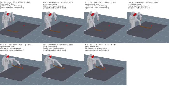
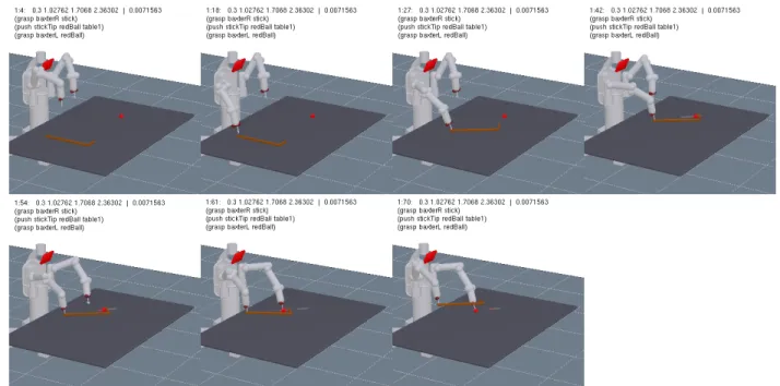
Fig 5.1.1 Example of a plan created by the system on a problem from the original

paper. The robot is given the stick in brown and tasked with grabbing the red ball placed outside of its reach. The plan shown here involves the robot picking up the stick and using it to tap the red ball toward itself.

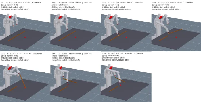
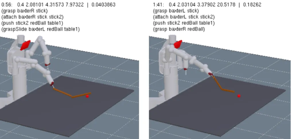
Fig 5.1.2 Example of a plan without new actions. The robot is given one long stick and is

tasked with acquiring the red ball. Here the robot has to awkwardly grasp the middle of the long stick to be able to use it to tap the red ball toward itself.

Fig 5.1.3 Example of the same problem as Fig 5.1.3 with the new attach and detach actions.

When rerunning original problems, comparisons were made on the time to find a first solution. First solutions are found earlier 24.3% of the time with the new actions added. The number of solutions found is higher with the new actions 29.7% of the

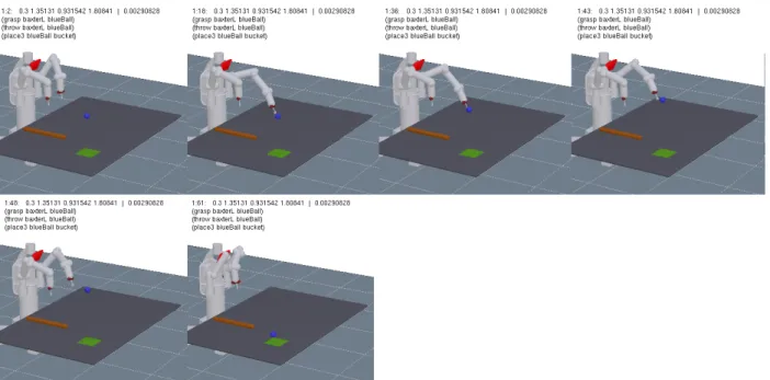
Fig 5.1.4 Example of a plan involving the robot throwing from an original paper problem. Here

the goal is to get the blue ball starting within the robots reach to the green target area. The solution shown involves the robot picking up the ball and tossing it to the target area.

Fig 5.1.5 Plot of Time vs # of solutions found for the same problem with and without new

actions. Here we can see that while with the new action a first solution is found earlier, It takes far longer for the search to terminate.

time, the same 67.4% of the time and less 2.9% of the time. The reduced time to find an initial solution likely is a result of solutions now possible with fewer actions. These solutions generally included a break early on.

anywhere along their length, the run time almost doubles. (Fig 5.1.5) Even when attach and break actions are restricted to small or recessed areas (see 4.4) the run time only showed a minor improvement. However, the quality of the attaches were, by human judgement, much more sturdy.

5.2 Recreating Tools from Tool Use Problems

The second class of experiments involves recreating problems like those in the original paper, except this the tools are broken into pieces. The pieces are then placed in a variety of positions, alignments and orientations. Additionally, experiments were run with pieces of various sizes.

Fig 5.1.6 The left picture shows an attach where the only requirement is two pieces

While in the original LGP system, the placement of the tool had only minor impact on the solutions generated, in the new system the placement of the same pieces of tools in different areas of a robot’s work space could change both the types

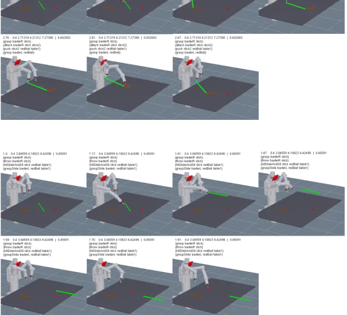
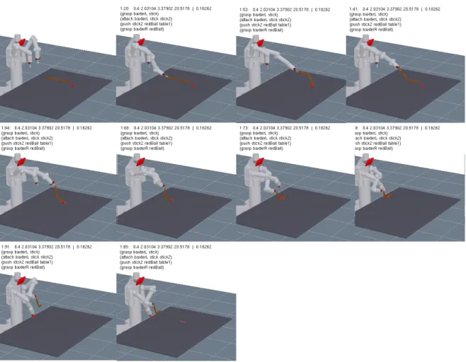
Fig 5.2.1 Example of a plan for an unmodified problem which serves as a base for

variations shown in later examples. Here the goal is for the robot to grasp the red ball.

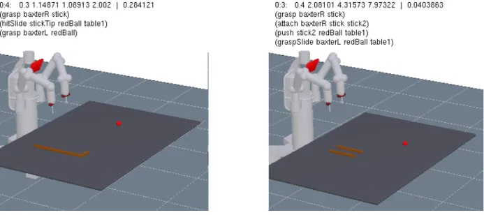
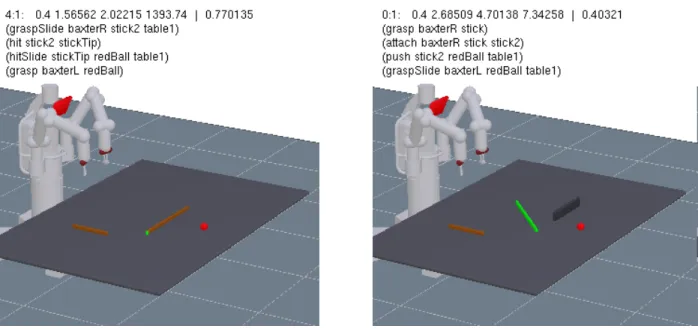
of solutions generated and the types of tools created. Comparing the solution in Fig 5.2.1 with that in Fig 5.2.2 we see that although the pieces are there, instead of creating the expected tool the system opts to use the smaller piece to hit the larger piece which in turn taps the red ball towards itself.

In a class of problems with two pieces of equal length, but neither long enough to reach a target object, a ball, often the solution was to attach one to the other to create a longer stick and push or tap the ball to itself. Where and how the two pieces started in relation to each other changed when the system found solutions, sometimes as much as 3x to find a first solution (Fig 5.2.4).

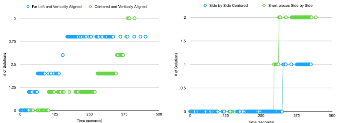
Fig 5.2.5 Plan created with two pieces side by side shifted slightly to the right. Fig 5.2.4 Comparison of when solutions are found when the pieces are shifted left

and right on the table. The left graph compares pieces vertically aligned and the right graph compares pieces that are placed side by side (horizontally aligned).

Fig 5.2.6 Plan produced when two pieces are vertically aligned and shifted left.

Fig 5.2.7 Comparison of when solutions are found when pieces are rotated around

each other. The left graph compares pieces aligned vertically with those place side by side. The right graph compares pieces place side by side with the same relative orientation rotated 90˚.

Fig 5.2.8 Plan produced when two pieces are side by side and rotated horizontally.

Fig 5.2.9 Comparison of plans when the the length of the pieces are altered. In

Not only were some orientations far less efficient to search through, some returned no solutions with attaches, preferring to instead throw, hit or slide the pieces at the ball despite both pieces being within reach of the robot. In these cases often the further piece was placed far enough away that an additional break and attach or grasp and place would’ve been necessary to create a tool shaped to reach the ball. Instead of taking the extra actions and movement the system found ‘better’ solutions by throwing or hitting.

Fig 5.2.10 Examples of problems that did not produce solutions with an attach or break.

Left: The remaining piece is near the edge of the robot’s workspace and to attach end-to-end is difficult. The piece would need to be moved closer first.

Right: The robot picked up the short end of the broken hook and would have to change hands or place and pick up again to use after making it via an attach.

5.3 Creating New Tools in Obstacle Problems

The final class of experiments added new obstacles or awkwardly pre-attached tools. Obstacles were designed with the intent to prevent the robot from simply using the existing pieces or pre-attached tools to find a solution. Problems were designed with the target object behind walls, in narrow slots, under blocks and placed on top of tall blocks. The robot is assumed to have knowledge of the world, obstacles and target object location.

Fig 5.3.2 Plans formed for a problem with a target object under a block. The second plan

involves throwing a piece through the added block and the table, despite collision costs incurred for both.

Fig 5.3.3 Plans found for a problem involving the target object placed high out of

reach. The second plan involves a path moving through the block, despite the costs of collision.

In creating new tools, the solver often struggled with balancing the search over action space and the incurred cost of moving through obstacles. As the original set of problems [1] generally had few obstacles (mainly just the table) the solutions often returned without collision. Likewise when recreating those problems with the tools starting in pieces, or awkwardly refigured, the robot was more often able to avoid collisions.

When creating new tools to get around obstacles, the system struggled to find good solutions. While the system could find collision free solutions for some problems, often it determined that moving very quickly through an obstacle was just as good or better than avoiding it. While the pieced together solution involved moving through obstacles, often the major waypoints of the path at the beginning and end of each action were collision free and could be used as a starting point for a more rigorous search involving hard collision constraints.

Fig 5.3.4 Both the old system (left) and the new system (right) struggled with solutions that

included collisions. In more open worlds, where the obstacle was not immediately blocked by an obstacle, these collisions were less frequent.

Like the previous LGP System, the new system also suffered from the simulator’s assumption of perfect execution and perfect physics. This resulted in solutions involving carefully thrown or hit pieces to result in a perfect trajectory for the target object. While some costs are added to even out the ability to overpopulate with only throwing or hitting solutions, the problems with added obstacles often saw solutions with objects being thrown or slid through them.

Fig 5.3.5 Examples of collisions with obstacles. Left shows a collision between a tool and

block and the image to the right shows the robot ignoring the tools on the table to reach through the obstacle instead.

Fig 5.3.6 Examples of solutions with objects being thrown. Right shows an object being slid

Even with the robot’s occasional tendency to move through obstacles instead of around them, the time to find a first solution was generally quicker in an environment with obstacles than without (Fig 5.3.7). This could be a result of the restricted space the robot has to operate in. Since the available moveable area is reduced by the obstacle, the possible orientations for an attach or break are much fewer and potentially quicker to optimize.

5.4 General Findings and Conclusions

The work here examines the results of adding two new actions, attach and break, to the existing LGP System for tool use [1]. The new system LGP for Tool

Creation was compared against the previous system on similar problems, as well as on new classes of problems that were previously unsolvable. The new solutions largely fall into two groups: recreating tools from previously seen problems and creating new types of tools in response to obstacles.

The addition of two new actions, attach and break, required surprisingly few changes to the original LGP formulation, and produced both new classes of results to existing problems as well as solutions to previously unsolvable problems. With the added actions the search generally runs for a longer amount of time, but when the new actions create shortcuts, or significantly better solutions, the time to first solution can decrease. However, the solutions produced by the optimization suffer from the use of a collision cost instead of a hard collision constraint and, depending on the problem, can often be infeasible due to collisions. Additionally, the placement of tools and pieces within a robot’s work area can greatly affect the type of solutions generated.

Fig 5.4.1 Comparison of time to find solutions across all problems. Here we can see

while minor changes to the problem’s start conditions do alter their run time, the far greater trend is due to the type of problem encountered.

Purple involves obstacle problems where obstacles were basically ignored. Blue shows runtimes of a few unaltered problems.

Green indicates problems similar to unaltered problems using the new actions. Yellow plots the variations of a broken tool with various starting poses.

5.5 Future Work

The approach here was to make minimal changes to the existing LGP system[1] to explore the solver’s flexibility on a new class of problems. To create more useable solutions with tool creation, the system could be readjusted to put more priority on stability and feasibility of the solution and less on the optimality of the solution.

However as the system is optimization based, tweaks in these areas will only improve solutions up to a point, and might come at significant cost tradeoffs.

Simple additions to make the solutions more real-world ready, would be to adjust the way obstacle costs are computed to be more strict. While too many constraints can cause the problem to be intractable, the current propensity of the system to move straight through obstacles could certainly be improved. A more complex change would be to incorporate a notion of uncertainty or guessed risk in executing certain actions. This could be done at first by hand by programmer for a small number of actions, or later computed on the fly by sampling from forward simulated mini plans using slightly tweaked initial poses or robot configurations.

The difficult part would be finding a good tradeoff between an acceptable added amount of security and the length of compute to get the plan. Currently plans of ~2-5 minutes take ~1-2 minutes to find a first possible solutions and ~2-4 to have at least 3 solutions to compare. If the robot assumes perfect, or near perfect completion it is somewhat feasible to be running constantly. However any significant detected deviation would require a break to begin replanning.

The other approach to getting world-ready would be to connect the proposed plan as a prior to a planner with stricter collision constraints. This might give good enough, although now non-optimal plans, within a reasonable amount of time. The solutions here generally dealt with a small number of pieces without any extraneous bits. Future work could look into the affect of having a box, or similarly large collection of pieces to work with. Similarly the tools here were used to complete only one task. It might be interesting to see what sort of tool might be created when presented with a task requiring the robot to potentially use two tools, or the the same tool twice.

Expanding, or redesigning the action set could also prove to be interesting For example simply removing the actions throw, hit or slide and adding more types of flexible joining, like bend. If new physical joints were defined perhaps simple mechanisms like springs could be used in tools to create different types of forces.

References

[1] M. Toussaint, K. R. Allen, K. A. Smith, and J. B. Tenenbaum: Differentiable Physics and Stable Modes for Tool-Use and Manipulation Planning. In Proc. of Robotics: Science and Systems (R:SS 2018), 2018.

[2] Peter Battaglia, Jessica Hamrick, and Joshua B Tenenbaum. Simulation as an engine of physical scene understanding. Proceedings of the National Academy of Sciences, 110(45):18327-18332, 2013.

[3] BBC Studios. “Wild crows inhabiting the city use it to their advantage - David Attenborough - BBC wildlife”. Online video clip. YouTube. YouTube, 12 February 2007. Web. 12 May 2018.

[4] Smolker, R. , Richards, A. , Connor, R. , Mann, J. and Berggren, P. (1997), Sponge Carrying by Dolphins (Delphinidae, Tursiops sp.): A Foraging Specialization Involving Tool Use?. Ethology, 103: 454-465. doi:10.1111/j.1439-0310.1997.tb00160.x

[5] Sanz, Crickette Marie, et al. Tool Use in Animals: Cognition and Ecology. Cambridge University Press, 2014.

[6] T. Siméon, J-P. Laumond, J. Cortes, and A. Sahbani. “Manipulation Planning with Probabilistic Roadmaps”. The International Journal of Robotics Research. vol. 23, no. 7-8, pp. 729-746. Aug 2004.

[7] Fabien Lagriffoul, Dimitar Dimitrov, Julien Bidot, Alessandro Saffiotti, and Lars Karlsson. Efficiently combining task and motion planning using geometric constraints. The International Journal of Robotics Research, 2014. doi:

[8] Igor Mordatch, Emanuel Todorov, and Zoran Popvic. Discovery of complex behaviors through contact-invariant optimization. ACM Transactions on Graphics (TOG), 31(4):43. 2012.

[9] Tomás Lozano-Pérez and Leslie Pack Kaelbling. A constraint-based method for solving sequential manipulation planning problems. In Intelligent Robots and Systems (IROS 2014), 2014 IEEE/RSJ International Conference On, pages 3684-3691. IEEE, 2014.

[10] L.P. Kaelbling and T. Lozano-Pérez. Hierarchical task and motion planning in the now. In Robotics and Automation (ICRA), 2011 IEEE International Conference On, pages 1470-1477, 2011.

[11] Siddharth Srivastava, Eugene Fang, Loreanzo Riano, Rohan Chitnis, Stuart Russell, and Pieter Abbeel. Combined task and motion planning through and extensible planner-independent interface layer. In Robotics and Automation (IRCA), 2014 IEEE International Conference On, pages 639-646. IEEE, 2014.

[12] Marc Toussaint and Manuel Lopes. Multi-bound tree search for logic-geometric programming in co-operative manipulation domains. In Proc. of the IEEE Int. Conf. on Robotics and Automation (ICRA 2017), 2017.

[13] Kris Hauser and Jean-Claude Latombe. Multi-modal motion planning in non-expansive spaces. The International Journal of Robotics Reserach, 29(7): 897-915, 2010.

[14] Robin Deits and Russ Tedrake. Footstep planning on uneven terrain with mixed-integer convex optimization. In Humanoid Robots (Humanoids), 2014 14th IEEE-RAS International Conference On, pages 279-286. IEEE, 2014.