HAL Id: inserm-00183785
https://www.hal.inserm.fr/inserm-00183785
Submitted on 31 Oct 2007HAL is a multi-disciplinary open access archive for the deposit and dissemination of sci-entific research documents, whether they are pub-lished or not. The documents may come from
L’archive ouverte pluridisciplinaire HAL, est destinée au dépôt et à la diffusion de documents scientifiques de niveau recherche, publiés ou non, émanant des établissements d’enseignement et de
Image reconstruction for positron emission tomography
using fuzzy nonlinear anisotropic diffusion penalty.
Hongqing Zhu, Huazhong Shu, Jian Zhou, Christine Toumoulin, Limin Luo
To cite this version:
Hongqing Zhu, Huazhong Shu, Jian Zhou, Christine Toumoulin, Limin Luo. Image reconstruction for positron emission tomography using fuzzy nonlinear anisotropic diffusion penalty.. Medical and Biological Engineering and Computing, Springer Verlag, 2006, 44 (11), pp.983-97. �10.1007/s11517-006-0115-4�. �inserm-00183785�
Image Reconstruction for Positron Emission Tomography Using Fuzzy
Nonlinear Anisotropic Diffusion Penalty
Hongqing Zhu1, Huazhong Shu1, 3, Jian Zhou1, 3, Christine Toumoulin2, 3, Limin Luo1, 3
1Lab. of Image Science and Technology, Department of Computer Science and Engineering, Southeast University, 210096 Nanjing, People’s Republic of China
2Laboratoire Traitement du Signal et de l’Image, Université de Rennes I – INSERM U642, 35042 Rennes,
France
3Centre de Recherche en Information Biomédicale Sino-français (CRIBs)
HAL author manuscript inserm-00183785, version 1
HAL author manuscript
Abstract: Iterative algorithms such as ML-EM become the standard for the reconstruction in emission
computed tomography. However, such algorithms are sensitive to noise artifacts so that the reconstruction begins to degrade when the number of iterations reaches a certain value. In this paper, we have investigated a new iterative algorithm for penalized-likelihood image reconstruction that uses the fuzzy nonlinear anisotropic diffusion as a penalty function. The proposed algorithm does not suffer from the same problem as that of ML-EM algorithm, and it converges to a low noisy solution even if the iteration number is high. The fuzzy reasoning instead of a nonnegative monotonically decreasing function was used to calculate the diffusion coefficients which control the whole diffusion. Thus, the diffusion strength is controlled by fuzzy rules expressed in a linguistic form. The proposed method makes use of the advantages of fuzzy set theory in dealing with uncertain problems and nonlinear anisotropic diffusion techniques in removing the noise as well as preserving the edges. Quantitative analysis shows that the proposed reconstruction algorithm is suitable to produce better reconstructed images when compared with ML-EM, OS-EM, Gaussian-MAP, MRP, TV-EM reconstructed images.
Keywords Fuzzy, Nonlinear anisotropic diffusion, Positron Emission Tomography (PET), Image
reconstruction, Maximum likelihood-expectation maximization (ML-EM)
1 Introduction
Iterative image reconstruction methods have attracted considerable attention in the past decades for applications in positron emission tomography (PET) due to the feasibility of incorporating the physical and statistical properties of the imaging process more completely [4, 25]. So far, all statistical reconstruction algorithms are based on the maximum likelihood (ML) or the least squares cost function. The maximum likelihood-expectation maximization (ML-EM) algorithm [31], which is a general statistical method for seeking the estimate of the image, allows computing projections that are close to the measured projection data. Iterative based ML reconstruction algorithms nevertheless require a considerable computational cost per iteration. An accelerated version of the ML-EM algorithm, the ordered subsets EM (OS-EM) was proposed by Hudson et al. [21] to significantly improve the convergence speed in the PET reconstruction. This ordered subset principle has been then exploited in many algorithms for the same objective. Let cite for instance the rescaled block-iterative EMML algorithm (RBI-EMML) [7], the row-action ML algorithm (RAMLA) [6], the complete-data OSEM (C-OSEM) [19] or the paraboloidal surrogates (PS) method (OS-SPS) [1].
Generally speaking, the tomography reconstruction with a limited number of data appears as a highly underdetermined ill-posed problem. The projection data generated by the PET system are initially noisy and the ML algorithm tends to increase this noise and in particular the noise artifacts through the successive iterations. This accumulation of noise leads to a premature stopping of the ML-EM reconstruction process. Several methods have been developed to decrease this accumulation of noise and improve the quality of the reconstructed images in tomography [32, 9, 23, 15]. Some include a penalty function (they are also called regularization techniques) to control the noise propagation and produce a satisfactory reconstruction. This is the case of the Maximum a Posteriori (MAP) algorithm based on the Bayes theorem [17, 18, 12]. The MAP solution can be found by combining the Poisson likelihood function with the image prior. MAP algorithms lean on local characteristics such as the nearest neighbor correlation or the homogeneity in the local neighborhood to decrease or remove the noise and smooth the reconstructed image. The one-step-late algorithm, introduced in the field of image reconstruction by Green [18], has the particularity to exploit the previous iteration to compute prior coefficients. The MAP
estimation allows the introduction of a prior distribution which reflects the likelihood of the estimate. However, if no prior distribution is available, another solution is to design an edge-preserving image mode as a prior distribution. A wide variety of methods have been reported in the literature that include edge-preserving techniques such as the Gibbs prior [17], entropy prior [12], median root prior (MRP) [3, 9, 32], Huber prior function [9, 14] and total variation (TV) prior [27]. The Gibbs prior assumes the Markov random field distribution for emitted photons. The entropy prior is based on the classical Boltzmann statistics for emitting particles (atoms or molecules) [12]. The MRP assumes that the unknown image is locally monotonic, i.e., the pixel values are spatially non-increasing or non-decreasing in a local neighborhood. This kind of method may not be very accurate in some cases [9], but is suitable to use when the image resolution is high. The Huber prior function proposed by Fessler [14] has a shape similar to the log (cosh (t)) used by Green [18]. It provides accurate and low noise images, but the parameters (the regularized parameter β and threshold parameterδ ) may be difficult to determine. Panin et al. [27] shown that the TV-EM algorithm using the total variation as a penalty term, was quite effective for SPECT. Nevertheless, the TV penalty term may include some bias in the reconstruction and reduce the contrast of the resulting image [27]. Another class of iterative image reconstruction methods made use of the weighted least squares (WLS) method [4, 13]. Recently, Anderson et al [4] developed a WLS algorithm and demonstrated that this algorithm converged faster than the ML-EM and produced images that were significantly of better resolution and contrast.
Since the introduction of fuzzy set theory by Zadeh in 1965 [36], the fuzzy theory and applications have been rapidly developed in the areas of image processing and computer vision, such as filtering [33], enhancement [30], and segmentation [24]. However, there is few research dealing with emission tomography problems until recently. A fuzzy clustering-based segmentation technique was applied in [37] to segment the transmission images into the main anatomical regions of the body in terms of the corresponding attenuation coefficient values. This approach allows to reduce the noise in the correction maps while correcting for attenuation coefficients of specific tissues. In [26], a fuzzy rule was included in a MAP algorithm, where the potential function was modeled on the basis of fuzzy derivatives and fuzzy rules. It was shown [26] that the method is very effective to remove the noise without destroying the
useful information contained in the reconstructed image.
The aim of this paper is to propose a new penalized likelihood iterative reconstruction algorithm for PET, based on a fuzzy non-linear anisotropic diffusion to remove noise while avoiding over-smoothing across edges. The nonlinear anisotropic diffusion (AD) process has shown the capability of eliminating the noise while preserving the accuracy of edges and, has thus been widely used in image processing [28, 22, 29]. In Perona-Malik diffusion [28], a non-negative and monotonically decreasing function which approaches zero at infinity was used, so that the diffusion process takes place only in the interior of regions. It thereby does not affect the edges where the magnitude of the gradient is sufficiently large. This non-negative and monotonically decreasing function is also called as diffusion coefficient. Demirkaya [10] proposed a method to suppress the streak artifacts and reduce the statistical noise in the measured attenuation data in PET by filtering the 2D projections with a nonlinear AD filtering techniques. In [11], the AD filtering technique was used to denoise the emission images and the attenuation maps of a whole body and improve the quantitative accuracy of the emission images. Jin et al. [22] developed an adaptive nonlinear diffusion algorithm to filter the medical images by utilizing the Central Limit Theorem to select the threshold. Black et al. [5] expressed the idea that the choice of the diffusion coefficients could greatly affect the level of preservation of the edges. On the other hand, for noisy images, edge preserving and smoothing operations are combined in the same process. The former aims at preserving the intensity invariability of the edge pixel, while the latter aims at reducing the increase in noise. Fuzzy reasoning has demonstrated its efficiency in modeling these uncertainly problems [8]. In [8], the fuzzy reasoning has been used to calculate the diffusion coefficient and get a more accurate and flexible control of the smoothing and edge preserving. The diffusion process depends on the difference between the center pixel gray levels and neighbor pixel gray levels. It is limited on the edges by assigning a small diffusion coefficient when an edge is detected. On the contrary, the diffusion coefficient is large when a fast diffusion is needed, i.e., inside the regions. Here, we propose a new method from [8] to remove the noise while preserving the edges for the PET reconstruction which combines a fuzzy reasoning with a non-linear anisotropic diffusion to adapt the diffusion coefficients according to the characteristics of the image. We show that this new version does not suffer from the noise accumulation problem encountered
in the ML-EM algorithm and converge to a low noisy solution even if the iteration number is high
2 Materials and methods 2.1 Theoretical background
Shepp and Vardi [31] introduced a Poisson model that is widely accepted as being mathematically valid for the PET reconstruction process. In that model, the positron emissions are modeled as a spatial inhomogeneous Poisson process with unknown intensity. Given the measured emission data vector ={yi;
i = 1, ..., m}, the log-likelihood function to be maximized with respect to the activity ={xj; j = 1, ..., n} is
y x
∑
−
=
i i i iy
y
y
L
(
x
)
(
log
(
x
)
(
x
))
(1) where∑
+
=
j ij j i ip
x
r
y
(x
)
(2)pijdenotes the element of the system probability matrix P and represents the probability that a particle
emitted at pixel j will be detected by a detector pair i. designates the mean number of background noise counts in the ith measurement.
i
r
The goal of the PET reconstruction is to estimate the image vector x from the collected data vector y. The iterative expectation maximization (EM) algorithm starting with a strictly positive vector x(0) to
estimate an image by maximizing the log-likelihood function is given by:
∑ ∑
∑
=
+ i l il lk i ij i ij k j k jx
p
y
p
p
x
x
( ) ) ( ) 1 ( (3)where k is the iteration number.
The nonlinear anisotropic diffusion was introduced by Perona and Malik as an alternative to Gaussian (or low-pass) filtering [28]. Let us consider the following penalized functional U(x) defined on the spaces of smooth images Ω ∇ =
∫
Ω d U(x)ϕ
(|| x||) (4)where ∇ denotes the gradient operator,
|| x
∇
||
is the gradient magnitude, andϕ
(|| x
∇
||)
is a monotonically increasing function of|| x
∇
||
. One way to compute the above expression is via gradientdescent by using the calculus of variations theory ⎥ ⎦ ⎤ ⎢ ⎣ ⎡ ∇ ∇ ∇ ⋅ ∇ = = ∂ ∂ || || ||) (|| ' ' ) , , ( x x x ϕ U t t v u x (5)
with the initial and boundary conditions
0
)
0
,
,
(
u
v
=
x
x
, and =0 ∂ ∂ Ω ∂ N x (6)where ∇⋅ is the divergence operator, and N the outward unit norm of the boundary . We define a function g(x) such as Ω ∂
x
x
x
)
'
(
)
(
≡
ϕ
g
(7) Substitution of (7) into (5) yields]
||)
(||
[
)
,
,
(
x
x
∇
∇
⋅
∇
=
∂
∂
g
t
t
v
u
x
(8) Function g(⋅) represents the edge-stopping function or diffusion coefficient, this function is a nonnegative monotonically decreasing function with g(0) =1.0 and g(b)→0 when b→∞. Qualitatively, the effect of the anisotropic diffusion is to smooth the noisy on the image while preserving the edges. The diffusion processing can be controlled by the choice of diffusion coefficient g(⋅) that greatly affects the extent to which discontinuities are preserved. Eq. (8) can be discretized as follows:t v u W W E E S S N N t v u t v u x C x C x C x C x x 1 , , , = + [ ⋅∇ + ⋅∇ + ⋅∇ + ⋅∇ ] +
λ
(9)where , , , are the diffusion coefficients in the direction north, south, east, west, respectively, and the parameter λ is chosen as
N
C CS CE CW
4 / 1
0≤
λ
≤ to ensure the numerical stability [28]. A simple method to approximate these diffusion coefficients is as follows:||)
(||
u,v 1 u,v Ng
x
x
C
=
−−
||)
(||
u,v 1 u,v Sg
x
x
C
=
+−
||)
(||
u 1,v u,v Eg
x
x
C
=
+−
||)
(||
u 1,v u,v Wg
x
x
C
=
−−
(10)Aja et al. [2] thought that these diffusion coefficients could be replaced by some fuzzy variables. The input parameters are the linguistic variables D1 and D2, and the output parameter is diffusion coefficient
CF . The computation of the variables D1 and D2 is realized as follows: for CE, the
input parameter D1 is the absolute difference between the centre pixel and the east direction pixel of 4-neighbor pixels, e.g., . The D2 is defined as D2=max{
})
,
,
,
{
(
F
∈
W
N
S
E
|
|
1
x
u,vx
u 1,vD
=
−
+ 2 1 , 1 1 , 1|
|
2
1
+ + − + v−
u v ux
x
, 2 , 1 1 , 1|
|
x
u+ v−−
x
u+ v2
1
,|
x
u+1,v+1−
x
u+1,v|
22
1
}. The purpose for us to define the variable D2 using such a strategy is that we prefer consider the contribution of all pixels gray levels rather than that of some pixels gray levels as proposed in [2]. Similar calculations are made for west, north, and south directions. We will use these input parameters to make a fuzzy inference to calculate the output parameter CF.
Linguistic variables D1, D2, CF can be modeled by the setsℜ1,ℜ2,ℜCcontaining certain number of terms described by fuzzy sets ℜ1σ,
ℜ
2
ς, ℜCυ}
,
,
,
,
,
,
,
{
}
1
,
,
1
,
,
1
{
1
1
1 8SS
SM
SL
MS
ML
LS
LM
LL
D
=
Δℜ
=
ℜ
L
ℜ
σL
ℜ
=
} , , , , , , , { } 2 , , 2 , , 2 { 2 2 1 8 SS SM SL MS ML LS LM LL D =Δℜ = ℜ L ℜ ς L ℜ =}
,
,
,
,
,
,
,
{
}
,
,
,
,
{
C
1C
C
8LL
LM
LS
ML
MS
SL
SM
SS
C
C
F=
Δℜ
=
ℜ
L
ℜ
υL
ℜ
=
(11)where the inputsℜ1σ,
ℜ
2
ς, and the output ℜCυ are defined as}
1
1
|
))
1
(
,
1
{(
1
=
D
1D
D
∈
ℜ
⊂
U
1ℜ
σμ
ℜσ ,σ
=
1 L
,
,
8
} 2 2 | )) 2 ( , 2 {( 2 = D 2 D D ∈ℜ ⊂U2 ℜ ςμ
ℜ ς ,ς
=
1 L
,
,
8
}
|
))
(
,
{(
C
F CC
FC
FC
U
cC
=
∈
ℜ
⊂
ℜ
υμ
ℜ υ ,υ
=
1 L
,
,
8
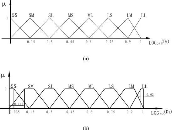
(12) The number of terms in each term set is 8; SS= small small, SMΔ = small medium, SL small large, ΔMS medium small, ML
Δ = Δ
= = medium large, LSΔ = large small, LMΔ = large medium, LL large large Δ are fuzzy numbers on the university sets U1(D1), U2(D2). Fig. 1(a) and (b) shows the membership functions with
triangular form and trapezoidal form, respectively. In the above definition,
Δ =
) (
τ
μ
SS is the membershipfunction associated with SS, where
τ
stands forD1 U∈ 1,D2 U∈ 2, CF ∈Uc. The membership function)
(
FCυ
C
μ
ℜ has the same form asμ
ℜ1σ(D
1
)
andμ
ℜ2ς (D2))
F
C
, the only difference being the x-axis which is
expressed as a function of 0.25*log10(10000− instead of log . Here, we assume that the
membership functions are analytically known from Fig. 1.
) 1 ( 255 D
The next step consists of setting the if … and … then rules of inference. We use the following fuzzy
rule in this algorithm
then CF is ℜCυ ς
2
ℜ
σ 1 ℜ R(D1, D2): If D1 is and D2 isThe rule set for the fuzzy anisotropic diffusion is based on the following idea: If the difference between the pixel gray levels is small, then the diffusion coefficient is high. On the contrary, a large restriction to diffusion is imposed when the difference is large enough. Table 1 shows this fuzzy anisotropic diffusion decision table: if … and … then rules. The content of the decision table can be modified according to the
characteristic of noise [2]. If FP-EM reconstructed images are characterized by a high level of noise, a larger diffusion coefficient is applied that emphasizes the smoothing inside the regions of the image. The decision table is thus built in such a way ℜCυ includes larger values of υ to take into account the high level of noise.
There are several ways to perform the operation of defuzzification. Some existing methods for defuzzification take into consideration the shape of the clipped fuzzy numbers. Here, we chose the mean of the maximum method proposed in [35].
2.2 Implementation of algorithms
In ML-EM, the objective function is based on the conditional probability , where y is the measured data, and x is the emission image. The penalized solution is of the form
)
|
(
y
x
f
xˆ
))
(x
(
max
arg
0 xˆx
ψ
≥=
(13) where)
(
)
(
)
(
x
=
L
x
+
F
x
ψ
(14) Here L(⋅) is the log-likelihood function and F(⋅) is the penalty term. In Bayesian terms, (13) represents the a posteriori probability and F(⋅) is the prior term resulting from the a prioriprobability . A commonly used Bayesian prior is the Gibbs distribution.
) ( ) | ( ) | (x y f y x fF x f ∝ ) (x F f
The purpose of this paper is to compute a penalized-likelihood estimate by replacing the function
F(⋅) in Eq. (14) by a fuzzy nonlinear anisotropic diffusion penalized function. The reconstruction method (called FP-EM) includes thus two terms: a log-likelihood term and a fuzzy penalty term. The estimate is then obtained by maximizing the function:
xˆ
xˆ
)
(
)
(
)
(
x
L
x
β
U
x
ψ
=
+
(15) where U(x) characterizes the penalty function defined in Eq. (4) and β the regularization parameter that balances between the goodness of the fitting to the original image and the amount of penalty imposed to the original image. The log-likelihood function L(x) can be written under the vector form as:) log( ) ( ) (x =−1T Px+r +yT Px+r L (16)
The first partial derivative of
ψ
(x
)
for each given pixel xj is as follows:) ( ) || || ||) (|| ' ( ) ( ) ( ) ( 1 r Px y P x x x x x x x x x − + + ∇ ∇ ∇ ⋅ = ∂ ∂ + ∂ ∂ = ∂ ∂
ψ
Lβ
Uβ
divϕ
T (17)The Kuhn-Tucker conditions for xj to be the optimal solution of the nonlinear optimization problem
imply: 0 ) ( = ∂ ∂ j x x
ψ
, ifx
j>
0
(18) 0 ) ( > ∂ ∂ j x xψ
ifx
j=
0
(19) The optimization of the functionψ
(x
)
can then be performed through a scale gradient descent algorithm. Finally, we derived the following iterative relation for computing the estimated image x:
(
)
)
||
||
||)
(||
'
(
( ) ( ) ) ( ) ( ) ( ) 1 (r
Px
y
P
x
x
x
P
x
x
+
∇
∇
∇
⋅
−
=
+ k T k k k T k kdiv
ϕ
β
(20)The above formula can be simplified by using (7) as follows:
) ( ) ||) (|| ( ( ) ( ) ( ) ) ( ) 1 ( r Px y P x x P x x + ∇ ∇ ⋅ ∇ − = + k T k k T k k g
β
(21)In image restoration, the diffusion coefficient g(⋅) is usually calculated by two nonnegative monotonically decreasing functions, i.e.,
)
)
||
||
(
exp(
||)
(||
2ε
x
x
=
−
∇
∇
g
(22) or 2 ||) / (|| 1 1 ||) (||ε
x x ∇ + = ∇ g (23)The constant ε takes a suitable tuning value whose setup can be obtained from the previous noise estimation. The equation above indicates that we could utilize the method described in subsection 2.1 to compute the diffusion coefficients.
2.3 Phantom description
We used a 128×128 pixel Shepp-Logan phantom that we downloaded from the web site [20] to evaluate the method in term of quality of the reconstruction and robustness to the noise (Fig. 2(a)). The simulated projections were calculated from such geometrical definitions as was the discrete representation of the phantom. The image is projected at 128 evenly spaced angles from 0 to 1800 with 128 samples per angle. The size of the final reconstructed image was 128×128 pixels. A stochastic Poisson noise was also added to the simulated projections to reproduce a low SNR. Complicating factors such as attenuation and scatter were not considered in this study. The probabilities in the system matrix were computed in advance using the “angle of view” method proposed in [31]. Two sinograms were designed to test the algorithm: a noiseless one and another one noisy, this latter being generated by adding to the original projection data a uniform field of random coincidences reflecting a scan of 6% of the total counts [16].
These two sinograms were globally scaled to a mean sum of 1,000,000 true events.
Fig. 2(b) depicts another phantom on which we compared the performances of the algorithm in presence of two kinds of noise: Poisson and Gaussian noise. It represents an elliptic uniform disc, two cold spots, and two hot spots of different diameters included in the internal structure of the disc. The size of the image matrix is 384×384 mm2 and the pixel size is 3 mm. The projection data were obtained from a forward projection of the phantom. These projection data were arranged into 180 angular views, each view consisting of 128 parallel lines of response (LORs). Two noisy sinograms were also built to test the algorithm, respectively including a Poisson (2×10⁵ photons) and a Gaussian noise (zero mean and 0.005 variance).
2.4 Evaluation of the reconstruction quality
The performance of the algorithm was evaluated from four objective criteria:
• The Log-likelihood function. Since the proposed algorithm computes iteratively the estimate of the penalized likelihood, the log-likelihood function was an appropriate qualitative measure to assess the performance of the algorithm. The log-likelihood function is given by Eq. (1).
• The normalized Mean Square Error (MSE). We measured the convergence rate by computing the normalized mean square error (MSE) between the simulated noiseless activity distribution and the image estimate as a function of the iteration number k. This item expresses the dispersion between the reconstructed image and the original phantom. The definition of the MSE is given by:
2 2 ) ( || || || || true true k MSE x x x − = (24) where ||⋅||2 is the standard Euclidean norm. xtrue and x(k) denote the value of the simulated activity image vector and the reconstructed image vector, respectively.
• The bias of a region of interest (ROI). The intensities on the phantom under consideration is assumed to be constant over each ROI and equal to true
ROI
x . Let x(ROIk) be the mean intensity over a ROI, then the Bias on a
ROI is defined as follows [27]: true ROI true ROI k ROI Bias x x x − = ( ) (25)
• The variance on a ROI. The variance measure is also used to evaluate the quality of the reconstruction:
∑
∈ − − = ROI j k ROI j x N Variance ( ( ) )2 1 1 x (26)where N denotes the number of pixels in the ROI.
3. Results
Images have been reconstructed with six algorithms: the maximum likelihood-expectation maximization algorithm (ML-EM), the OS-EM [21], the Maximum a Posteriori reconstruction algorithm with Gaussian prior (Gaussian-MAP) [18], the prior based on the median filter: MRP [3], the Maximum a Posteriori with total variation energy potential (TV-EM) [27] and our algorithm called FP-EM. The initial estimator x(0) was set to a strictly non-zero positive vector. For Gaussian-MAP, MRP, TV-EM, and the FP-EM, the regularization parameter β was set to 1, 0.5, 0.8, and 1, respectively, and was kept constant over the iterations. The triangular membership function shown in Fig. 1(a) was used for FP-EM.
Fig. 3 shows the reconstruction results on the noiseless Shepp-Logan phantom using the different methods. Except for the OS-EM algorithm, the iteration number was fixed to 100 for all the reconstructions. For the OS-EM reconstruction, the number of iterations was set to 8 with 4 subsets. A first visual analysis shows that the ML-EM reconstruction provides a satisfactory result but is characterized by a slightly streaky artifacts inside the object (Fig. 3(a)), the OS-EM method globally increases the contrast of the reconstructed image (Fig. 3(b)), the Gaussian MAP and MRP algorithms leads to an over smoothing on the reconstruction (Fig. 3(c), (d)), the TV-EM and the FP-EM reconstructions globally provides a good reconstruction of the image but make appear a very slightly blurring along the edges (Fig. 3(e), (f)).
Simulations were then performed on noisy projection data. Fig. 4(a) shows the reconstruction
obtained by stopping the ML-EM algorithm at iteration 25 (corresponding to the smallest MSE). In the case of a non-penalized ML-EM and OS-EM, the remaining noise inside the object is higher than in the result obtained from the Gaussian MAP method. Moreover, this noise increases with the number of iterations. The background in the resulting MRP reconstruction is more uniform than in the Gaussian-MAP’s. However, the cold spot of MRP was contaminated by more noise compared to the Gaussian-MAP's. When introducing the penalty term in the TV-EM formulation, the result makes appear a good reduction of the noise as an edge preservation although a small bias along the edges. The FP-EM algorithm has a better behavior to the noise compared with the other methods: regions have been well smoothed and the sharp edges as the small artifacts of oscillatory nature have been significantly reduced.
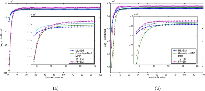
Fig. 5 depicts the convergence speed for the reconstructed images by the log-likelihood function. Although the log-likelihood function with TV-EM algorithm increases rapidly at the early iterations, as can be seen in the enlarged part, the FP-EM algorithm has better behavior in terms of convergence with increasing iteration number. It is also observed that the MRP algorithm has better performance than the TV-EM, Gaussian-MAP and ML-EM algorithms. Comparing the results presented in Fig. 5(a) and (b), one can see that the log-likelihood functions of the image reconstructed from noisy projections are in good agreement with the case of projections without noise. The simulation results obtained with the proposed algorithm show a significant improvement in convergence rate.
Detailed comparisons of MSE of reconstruction using noiseless projections and noisy projections are shown in Fig. 6(a) and (b), respectively. Fig. 6 illustrates the stability of the FP-EM algorithm in comparison with the ML-EM, Gaussian-MAP, MRP, TV-EM algorithms. The ML-EM algorithm converges to maximal-likelihood image, which, however, is not the desired solution due to the high noise level. In our simulation, the MSE in ML-EM reconstruction reaches its minimum at iteration number 25 and then starts to increase with increasing iteration number. In other words, it should be stopped after a certain number of iterations, e.g. iteration 25. However, the proposed FP-EM method does not suffer from this shortcoming and it converges to a low noisy solution even if the number of iterations is high. The MRP and TV-EM reconstructions have also better quality than ML-EM and Gaussian-MAP reconstructions according to the simulation of mean square errors.
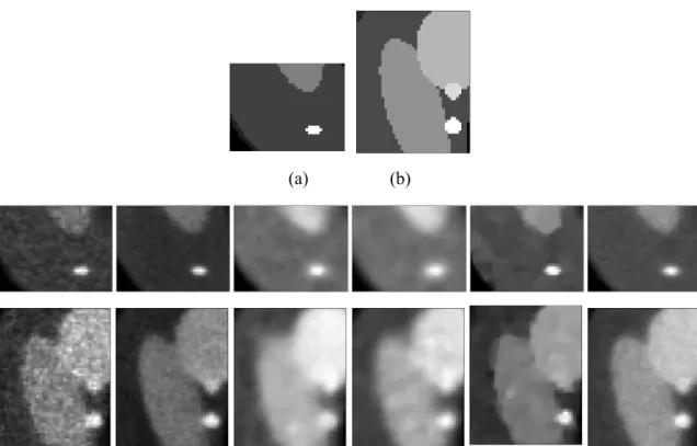
A portion of the reconstructed Shepp-Logan phantoms has been zoomed in Fig. 7. From a visual standpoint, the ML-EM images suffer from the presence of noise compared to the other images. In contrast, one can observe that Gaussian-MAP reconstructed images are too smooth, especially nearby the boundary of the different tissues. The OS-EM reconstruction was characterized by the highest contrast recovery of spots and high noise level. From Fig. 7, we see that the noise was removed from the interior regions of TV-EM image but it is still present along the edges. On the other hand, the fuzzy anisotropic diffusion regularization smoothes out the noise from the region interiors and preserves well the edges in the reconstructed images. To enhance this fact, we present another portion of the phantom shown in the third row of Fig. 7. It shows that the edges of the small spot in the TV-EM image are not as clear as the ones in the FP-EM image. In the reconstructed images with Gaussian-MAP, MRP, TV-EM, the small spot is completely removed from these images. Fig. 7 illustrates that the FP-EM image is smooth and, at the same time, two spots in the image are well reconstructed and differ greatly from the background.
Fig. 8 shows the same profiles of the Shepp-Logan phantom for six different reconstruction methods to further evaluate the proposed iterative algorithms in terms of the image quality. The projection data include 6% uniform Poisson distributed background events. ML-EM and OS-EM profiles show that these methods are more sensitive to the noise (see Fig. 8(b), (c), (e)), they increase the noise making the regions inhomogeneous. Gaussian-MAP, MRP and TV-EM tend to significantly increase the intensity inside the regions. MRP and FP-EM profiles appear close to the initial profile drown on the phantom (Fig. 8(b), (c), (d)). In terms of the spike (pixel position 65, Fig. 8(d)), only the FP-EM method keeps a close profile to the initial one even if it gives a slight of the intensity. The others give either a more important under-estimation (OS-EM, TV-EM, ML-EM) or an over-estimation (MRP, Gaussian MAP). These results are consistent with the visual observation of the hot spots in the reconstructed phantom shown Fig. 4. In conclusion, the method that better preserves the edges while smoothing the region is the FP-EM method. We now consider the case where the projections include a 6% uniform Poisson distributed background
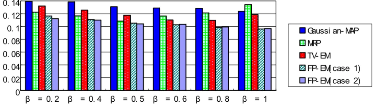
events. Fig. 9 depicts the MSE values for a set of four methods (Gaussian-MAP, MRP, TV-EM, and
FP-EM for which both the triangular form and trapezoidal form were used as the membership function) for different weightings of the penalty term (0.2 ≤ β ≤1). It can be seen that the quality of the MRP and
TV-EM reconstruction is slightly dependent on the parameter β, the lower MSE is obtained when β was selected 0.5 and 0.8, respectively. Larger β values in the MRP and TV-EM algorithms lead to the degradation of the image. FP-EM is insensitive to the changes of β when β∈[0.2, 1]. Even if a small weight is assigned to the penalty term (β = 0.2), FP-EM gives a lower MSE than those obtained by the other algorithms. Gaussian-MAP provides its lowest MSE for β = 1. These experiments show that MRP, TV-EM, Gaussian-MAP, and FP-EM give the best reconstruction when β is set to 0.5, 0.8, 1, and 1, respectively. This graph also shows that the use of one or the other membership function does not change the performance of the FP-EM method.
To further test the robustness of the proposed method regarding to different kinds of noise and different phantoms, we examined the behaviors of FP-EM method using a phantom containing a cold and hot spots shown in Fig. 2 (b). The reconstruction was stopped after 40 iterations. For OS-EM method, 4 subsets were used. We first test the robustness of the proposed method under Poisson noisy conditions shown in the first row of Fig. 10. The results again indicate the better performance of the FP-EM for Poisson noisy projection data. The reconstructed images using noisy projections contaminated by zero mean Gaussian noise with variance 0.005 were shown in the second row of Fig. 10. One can observe that the OS-EM and TV-EM reconstruction decrease the contrast of reconstructed images, especially in the lower activity area. This phenomenon is more obvious for OS-EM. MRP algorithm effectively alleviate the noise artifacts in the reconstructed images, however, MRP has slightly poorer capability to preserve the edges. Gaussian-MAP or FP-EM seems to reach a good compromise between the noise suppression and loss of spatial resolution, at least from a visual standpoint.
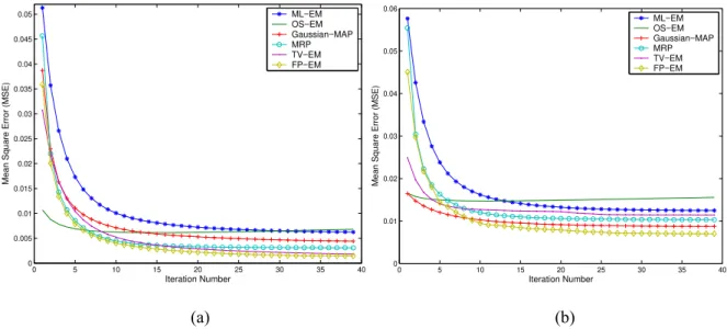
Fig. 11(a) and (b) display the detailed plot of the MSE using six different algorithms with maximum iteration number up to 40 under different noisy projection conditions. As it can be seen from Fig. 11, the OS-EM (4 subsets) converges faster than other algorithms at early iterative steps. It achieves the minimum MSE value at iteration 8 then this value re-increases with increasing iteration number. Fig. 11(a) shows that FP-EM has the best performance in terms of the robustness to Poisson noise, and the TV-EM performs better than the Gaussian-MAP, MRP, EM-EM and OS-EM methods. However, we can see from Fig. 11(b) that, for projection data contaminated by Gaussian noise, the TV-EM did not perform as well as
for Poisson noisy projections. MRP seems to be quite insensitive to this kind of noise. Due to the use of MRP prior, noises can be effectively suppressed in the reconstructed image, but the edges were blurred as shown in Fig. 10.
Tables 2, 3 and 4 tabulate the variance of the ROIs with different activities. For Poisson noisy projections: projections including 2×10⁵ photons uniform Poisson distributed background noises. For
Gaussian noisy projections, projections contained by zero mean value Gaussian noise with variance 0.005.
Variance analyses are consistent with those of visual observation of the hot spots and cold spots in the reconstructed image shown in Fig. 10, and consistent with those of MSE analysis indicated by Fig. 11.
In Fig.12, we discuss the bias on the ROIs with different activities under Poisson and Gaussian noisy projection conditions shown in the first row and the second row, respectively. It can be observed from the first row that FP-EM displays the lowest bias for two ROIs. The bias appeared in the result with FP-EM for a ROI with medium background activity was only larger than that of MRP. Besides the FP-EM method, the TV-EM presents a smaller bias on the ROI with high activity compared to Gaussian-MAP, MRP, EM-EM and OS-EM algorithms, while the MRP has a better behavior in the low and medium activities. The experiment was repeated by using the Gaussian noisy projections to reconstruct the image. Among all the algorithms, the MRP gives the smallest bias on the ROI with low or medium activity, but it shows the biggest bias in the high activity. FP-EM reconstruction leads to the lowest bias ROI in higher activity.
4 Discussions
We have proposed a new iterative algorithm which exploits the fuzzy reasoning to calculate the diffusion coefficients. The control of the diffusion by a set of rules allows adapting the diffusion coefficients according to the characteristic of noise present in the projections or reconstructed image. The decision table (Table 1) was built to emphasize the smoothness on the region when the noise is important. The future work will be oriented to the introduction of techniques for learning and tuning the rule-base from data [34].
Experiments have shown that the FP-EM algorithm had good properties of convergence and that it was robust to the Poisson noise. On the other hand, a small bias can appear in presence of a Gaussian noise.
We have also shown that the choice of the regularization parameter β was critical for the Gaussian-MAP, MRP and TV-EM methods but not for the FP-EM (in this study, we selected a β value which provided the lowest MSE for each algorithm).
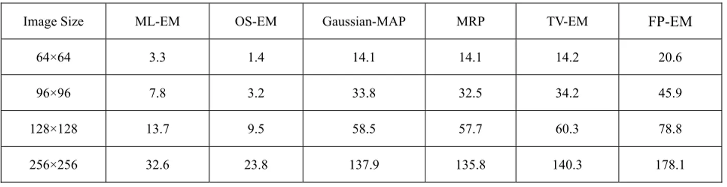
The FP-EM appears more expensive in terms of computation time (see Table 5). Note that the computer used in this experiment is Sony Corporation, VGN-S3 Series, Pentium (R), 1.8GHz, Memory: 1GB. Indeed, the ordered subset (OS) technique is a useful method to accelerate the image reconstruction for the ML-EM. OS-EM requires a less number of iterations than the other algorithms for achieving the convergence. However, like the ML-EM algorithm, the drawback of this method is the difficulty to remove the noise. If the iteration number is too high, the OS-EM produces a degraded image.
MRP has been used for the reconstruction of PET image and shown that it possessed a good noise reduction and in particular in presence of Gaussian noise. According to [3], if the median filter size in MRP is increased from 3×3 to 5×5, small edges may be smoothed. Therefore, we selected a median filter of size 3×3 to avoid an over-smoothing of the reconstructed image. However, Fig. 7 still indicates a risk in using MRP on small structures because they can be completely removed from the image.
The TV-EM algorithm is less robust to the Gaussian noise than to the Poisson’s one, but its overall performance is not very high compared to the other methods.
5 Conclusions
The ML-EM method is the most general statistical approach and becomes the standard in positron emission tomography. However, the reconstructed images become increasingly noisy as the number of iterations increases. To limit the noise accumulation, we have presented an iterative algorithm for PET reconstruction based on fuzzy anisotropic diffusion penalty. The proposed method is capable of taking advantages of fuzzy theory and anisotropic diffusion regularization. It appears more accurate compared to the ML-EM, OS-EM, Gaussian-MAP, MRP, and TV-EM algorithms. The fuzzy anisotropic diffusion penalty has an effect of edge-preserving and denoising. It allows suppression of noise and Gibbs phenomena without significantly affecting the edges. Simulation results showed that incorporation of the fuzzy anisotropic diffusion penalty improves the reconstruction quality for both noise-free and noisy
projection data.
Acknowledgement: This work was supported by National Basic Research Program of China under grant No. 2003CB716102 and Program for New Century Excellent Talents in University under grant No. NCET-04-0477. It has been carried out in the frame of the CRIBs, a joint international laboratory associating Southeast University, the University of Rennes 1 and INSERM, with a grant provided by the French Consulate in Shanghai. We thank the anonymous referees for their careful review and valuable comments to improve the quality of the paper.
References
1. Ahn S, Fessler JA (2003) Globally convergent image reconstruction for emission tomography using relaxed ordered subsets algorithms. IEEE Trans Med Imag 22:613-626
2. Aja S, Alberola C, Ruiz J (2001) Fuzzy anisotropic diffusion for speckle filtering. In IEEE Proc Int Conf Acoustics, Speech, and Signal Processing (ICASSP). 1261-1264
3. Alenius S. Ruotsalainen U (2002) Generalization of Median Root Prior Reconstruction. IEEE Trans Med Imag 21:1413-1420
4. Anderson JMM, Srinivasan R, Mair BA, Votaw JR (2005) Accelerated penalized weighted least-squares and maximum likelihood algorithms for reconstructing transmission images from PET transmission data. IEEE Trans Med Imag 24:337-351
5. Black MJ, Sapiro G, Marimont DH, Heeger D (1998) Robust anisotropic diffusion. IEEE Trans Image Processing 7:421-432
6. Browne JA, Pierro ARDe (1996) A row-action alternative to the EM algorithm for maximizing likelihoods in emission tomography. IEEE Trans Med Imag 15:687-699
7. Byrne CL (1998) Accelerating the EMML algorithm and related iterative algorithms by rescaled block-iterative methods. IEEE Trans Image Processing 7:100-109
8. Chen RC, Yu PT (1999) Fuzzy selection filters for image restoration with neural learning. IEEE Trans Signal Processing 47:1446-1450
9. Chlewicki W, Hermansin F, Hansen SB (2004) Noise reduction and convergence of Bayesian algorithms with blobs based on the Huber function and median root prior. Phys Med Biol 49:4717-4730
10. Demirkaya O (2002) Anisotropic diffusion filtering of PET attenuation data to improve emission images. Phys Med Biol 47:271-278
11. Demirkaya O (2004) Post-reconstruction filtering of positron emission tomography whole-body emission images and attenuation maps using nonlinear diffusion filtering. Acad Radiol 11:1105-1114 12. Denisova NV (2004) Bayesian reconstruction in SPECT with entropy prior and iterative statistical
regularization. IEEE Trans Nucl Sci 51:137-141
13. Fessler JA (1994) Penalized weighted least-squares image reconstruction for positron emission tomography. IEEE Trans Med Imag 13:290-300
14. Fessler JA (1997) Grouped coordinate descent algorithms for robust edge-preserving image restoration. In Proc. SPIE 97, Im Recon Restor II, 3170:184-194
15. Fessler JA, Ficaro EP, Clinthorne NH, Lange K (1997) Grouped-coordinate ascent algorithms for penalized-likelihood transmission image reconstruction. IEEE Trans Med Imag 16:166-175
16. Fessler JA, Hero AO (1994) Space-alternating generalized expectation-maximization algorithm. IEEE Trans Signal Processing 42:2664-2677
17. Geman S, Geman D (1984) Stochastic relaxation, Gibbs distributions, and the Bayesian restoration of Images. IEEE Trans Pattern Anal Machine Intell 6:721-741
18. Green PJ (1990) Bayesian reconstruction from emission tomography data using a modified EM algorithm. IEEE Trans Med Imag 9:84 – 93
19. Hsiao IT, Rangarajan A, Gindi G (2002) A provably convergent OS-EM like reconstruction algorithm for emission tomography. In proc. SPIE 4684, Medical Imaging 2002: Image Proc. :10-19
20. http://www.eecs.umich.edu/~fessler/code/
21. Hudson HM, Larkin RS (1994) Accelerated image reconstruction using ordered subsets of projection data. IEEE Trans Med Imag 13:601-609
22. Jin JS, Wang Y, Hiller J (2000) An adaptive nonlinear diffusion algorithm for filtering medical images. IEEE Trans Inform Technol Biomed 4:298-305
23. Kadrmas DJ (2001) Statistically regulated and adaptive EM reconstruction for emission computed tomography. IEEE Trans Nucl Sci 48:790-798
24. Kobashi S, Fujiki Y, Matsui M, Inoue N, Kondo K, Hata Y, Sawada T (2006) Interactive segmentation of the cerebral lobes with fuzzy inference in 3T MR image. IEEE Trans Syst Man Cybern B 37:74-86 25. Mondal PP, Rajan K (2004) Image reconstruction by conditional entropy maximization for PET
system. IEE Proc.-Vis. Image Signal Process 151:355-352
26. Mondal PP, Rajan K (2005) Fuzzy-rule-based image reconstruction for positron emission tomography. J Opt Soc Amer A 22:1763-1771
27. Panin VY, Zeng GL, Gullberg GT (1999) Total variation regulated EM algorithm. IEEE Trans Nucl Sci 46:2202-2210
28. Perona P, Malik J (1990) Scale-space and edge detection using anisotropic diffusion. IEEE Trans Pattern Anal. Machine Intell 12:629 – 639
29. Riddell C, Benali H, Buvat I (2004) Diffusion regularization for iterative reconstruction in emission tomography. IEEE Trans Nucl Sci 51:712 – 718
30. Russo F (2002) An image enhancement techniques combining sharpening and noise reduction. IEEE Trans Instrum Meas 51:824-828
31. Shepp LA, Vardi Y (1982) Maximum likelihood reconstruction for emission tomography. IEEE Trans Med Imag MI-1 (2):113-122
32. Sohlberg A, Ruotsalainen U, Watabe H, Iida H, Kuikka JT (2003) Accelerated median root prior reconstruction for pinhole single-photon emission tomography (SPET). Phys Med Biol 48:1957-1969 33. Ville DVanDe, Nachtegael M, Weken DVD, Kerre EE, Philips W, Lemahieu I. (2003) Noise reduction
by fuzzy image filtering. IEEE Trans Fuzzy Syst.11:429-435
34. Wang L-X, Mendel JM (1992) Generating fuzzy rules by learning from examples. IEEE Trans Syst Man Cybern 22:1411-1427
35. Yuan B, Klir G (1997) Fuzzy sets and fuzzy logic. Prentice-Hall International, New Jersey. 36. Zadeh LA (1965) Fuzzy sets. Information and Control 8:338-353
37. Zaidi H, Diaz-Gomez M, Boudraa AE, Slosman DO (2002) Fuzzy clustering-based segmented attenuation correction in whole-body PET imaging. Phys Med Biol 47:1143-1160
Table 1. Decision table of fuzzy nonlinear anisotropic diffusion rule. D2 D1 1 2 ℜ ℜ22 ℜ23 ℜ24 ℜ25 ℜ26 ℜ27 ℜ28 1 1 ℜ ℜC1 ℜC1 ℜC2 ℜC2 ℜC3 ℜC4 ℜC5 ℜC7 2 1 ℜ ℜC1 ℜC2 ℜC2 ℜC2 ℜC3 ℜC4 ℜC5 ℜC7 3 1 ℜ ℜC2 ℜC2 ℜC2 ℜC2 ℜC3 ℜC4 ℜC5 ℜC7 4 1 ℜ ℜC2 ℜC2 ℜC2 ℜC3 ℜC3 ℜC5 ℜC6 ℜC8 5 1 ℜ ℜC3 ℜC3 ℜC3 ℜC3 ℜC4 ℜC5 ℜC6 ℜC8 6 1 ℜ ℜC4 ℜC4 ℜC4 ℜC5 ℜC5 ℜC6 ℜC6 ℜC8 7 1 ℜ ℜC5 ℜC5 ℜC5 ℜC6 ℜC6 ℜC6 ℜC7 ℜC8 8 1 ℜ ℜC7 ℜC7 ℜC7 ℜC8 ℜC8 ℜC8 ℜC8 ℜC8
Table 2. The variance of a ROI with higher activity. The ROI contains 973 pixels.
Noise ML-EM OS-EM Gaussian-MAP MRP TV-EM FP-EM
Poisson 0.065941 0.072625 0.054043 0.054965 0.053571 0.053248
Gaussian 0.22759 0.20371 0.12704 0.14371 0.15842 0.11165
Table 3. The variance of a ROI with lower activity. The ROI contains 576 pixels.
Noise ML-EM OS-EM Gaussian-MAP MRP TV-EM FP-EM
Poisson 0.051018 0.053042 0.050012 0.051143 0.047039 0.049093
Gaussian 0.09265 0.09447 0.08142 0.08535 0.089048 0.07332
Table 4.The variance of in an ROI of medium activity. The ROI contains 4316 pixels.
Noise ML-EM OS-EM Gaussian-MAP MRP TV-EM FP-EM
Poisson 0.063541 0.072014 0.056213 0.051979 0.043026 0.041356
Gaussian 0.06147 0.06648 0.03391 0.04873 0.05391 0.03571
Table 5. The CPU time after 100 iterations for Gaussian-MAP, MRP, TV-EM and FP-EM algorithms (Second). 4 subsets and 8 iterations for OS-EM. 25 iterations for ML-EM (the smallest MSE was obtained)
Image Size ML-EM OS-EM Gaussian-MAP MRP TV-EM FP-EM
64×64 3.3 1.4 14.1 14.1 14.2 20.6 96×96 7.8 3.2 33.8 32.5 34.2 45.9
128×128 13.7 9.5 58.5 57.7 60.3 78.8
256×256 32.6 23.8 137.9 135.8 140.3 178.1
(a)
(b)
Fig. 1 Terms of linguistic variables D1, D2 (a) Triangle membership function. (b) Trapezoidal membership function
(a) (b)
Fig. 2 The phantoms used in the simulation study. (a) Shepp-Logan phantom (128×128 pixels). (b) Cold and hot spots phantom (128×128 pixels).
(a) (b) (c)
(d) (e) (f)
Fig.3 Images reconstructed from noiseless projection data using different methods. For OS-EM, 4 subsets and 8 iterations were used. For ML-EM, early stop at iteration 25 (the smallest MSE was obtained). (a) ML-EM algorithm (b) OS-EM algorithm (c) Gaussian-MAP algorithm (d) MRP algorithm (e) TV-EM algorithm (f) FP-EM algorithm
(a) (b) (c)
(d) (e) (f)
Fig.4 The Shepp-Logan phantom with different reconstruction methods. Projections including 6% uniform
Poisson distributed background events. For OS-EM, 4 subsets and 8 iterations were used. For ML-EM, early stop at iteration 25 (the smallest MSE was reached). (a) ML-EM algorithm (b) OS-EM algorithm (c) Gaussian-MAP algorithm (d) MRP algorithm (e)TV-EM algorithm (f) FP-EM algorithm.
0 10 20 30 40 50 60 70 80 90 100 0.95 1 1.05 1.1 1.15 1.2x 10 6 Iteration Number Log − Likelihood 5 10 15 20 25 1.13 1.14 1.15 1.16 1.17 1.18 1.19x 10 6 ML−EM Gaussian−MAP MRP TV−EM FP−EM 0 10 20 30 40 50 60 70 80 90 4.9x 10 5 100 4.4 4.5 4.6 4.7 4.8 Iteration Number Log − Likelihood 5 10 15 20 4.9x 10 5 25 4.7 4.75 4.8 4.85 ML−EM Gaussian−MAP MRP TV−EM FP−EM (a) (b)
Fig. 5 Comparison of log-likelihood function increase rates of ML-EM, Gaussian-MAP, MRP, TV-EM, and FP-EM algorithms. (a) Noiseless Projections (b) Projections including 6% uniform Poisson distributed background events. 0 10 20 30 40 50 60 70 80 90 100 0 0.005 0.01 0.015 0.02 0.025 Iteration Number
Mean Square Error (MSE)
5 10 15 20 25 30 0 0.001 0.002 0.003 0.004 0.005 0.006 0.007 0.008 0.009 0.01 ML−EM Gaussian−MAP MRP TV−EM FP−EM 0 10 20 30 40 50 60 70 80 90 100 0.05 0.1 0.15 0.2 0.25 0.3 Iteration Number
Mean Square Error (MSE)
ML−EM Gaussian−MAP MRP TV−EM FP−EM (a) (b)
Fig. 6 Comparative analysis of MSE versus iteration number. The MSE for the ML-EM, Gaussian-MAP, MRP, TV-EM, and FP-EM algorithms (a) Noiseless Projections (b) Projections including 6% uniform Poisson
distributed background events.
(a) (b)
Fig. 7 Close-up details of Shepp-Logan phantom. Projections include 6% uniform Poisson distributed background events. The iteration number was set to 100 for the Gaussian-MAP, MRP, TV-EM, and FP-EM. For OS-EM, 4 subsets and 8 iterations were used. For ML-EM, early stop at iteration 25 (the smallest MSE was reached). (a)(b) Synthetic phantom. From the first column to the last column are images with ML-EM, OS-EM, Gaussian-MAP, MRP, TV-EM, and FP-EM algorithm, respectively.
(a) 20 25 30 35 40 45 50 0.14 0.16 0.18 0.2 0.22 0.24 0.26 0.28 0.3 Pixel Position Intensity Phantom ML−EM OS−EM Gaussian−MAP MRP TV−EM FP−EM 30 35 40 45 50 55 60 0.4 0.45 0.5 0.55 0.6 0.65 Pixel Position Intensity Phantom ML−EM OS−EM Gaussian−MAP MRP TV−EM FP−EM 30 35 40 45 50 55 60 0.4 0.45 0.5 0.55 0.6 0.65 Pixel Position Intensity Phantom ML−EM OS−EM Gaussian−MAP MRP TV−EM FP−EM (b) (c) 56 58 60 62 64 66 68 0.56 0.58 0.6 0.62 0.64 0.66 0.68 0.7 0.72 0.74 0.76 Pixel Position Intensity Phantom ML−EM OS−EM Gaussian−MAP MRP TV−EM FP−EM 80 85 90 95 100 105 0.18 0.2 0.22 0.24 0.26 0.28 0.3 0.32 Pixel Position Intensity Phantom ML−EM OS−EM Gaussian−MAP MRP TV−EM FP−EM (d) (e)
Fig. 8 Error analysis of line profile at row 60. Projections including 6% uniform Poisson distributed background events. For OS-EM, 4 subsets and 8 iterations were used. The number of iterations was set to 100 for other algorithms. (a) The profiles of the six images reconstructed from Shepp-Logan phantom compared to the real pixel values. (b) - (e): Enlarged parts of (a).
0 0. 02 0. 04 0. 06 0. 08 0. 1 0. 12 0. 14 β = 0. 2 β = 0. 4 β = 0. 5 β = 0. 6 β = 0. 8 β = 1
Gaussi an- MAP MRP
TV- EM FP- EM( case 1) FP- EM( case 2)
Fig. 9 The MSE of Shepp-Logan phantom including 6% uniform Poisson distributed background events obtained by running 100 iterations for the Gaussian-MAP, MRP, TV-EM, and FP-EM algorithm using different regularization parameter β. Case 1: Triangle member function was used for FP-EM. Case 2: Trapezium membership function was used for FP-EM
Fig. 10 From the left column to the last column are respectively the ML-EM, OS-EM, Gaussian-MAP, MRP, TV-EM, and FP-EM algorithms. The first row is projection date contained by the Poisson noise. The second row is projection data contained by zero mean value Gaussian noise with variance 0.005.
0 5 10 15 20 25 30 35 40 0 0.005 0.01 0.015 0.02 0.025 0.03 0.035 0.04 0.045 0.05 Iteration Number
Mean Square Error (MSE)
ML−EM OS−EM Gaussian−MAP MRP TV−EM FP−EM 0 5 10 15 20 25 30 35 40 0 0.01 0.02 0.03 0.04 0.05 0.06 Iteration Number
Mean Square Error (MSE)
ML−EM OS−EM Gaussian−MAP MRP TV−EM FP−EM (a) (b)
Fig. 11 MSE versus iterations. (a) Projection contained Poisson noise. (b) Projection contained by zero mean value Gaussian noise with variance 0.005
0 5 10 15 20 25 30 35 40 1.4 1.6 1.8 2 2.2 2.4 2.6 2.8 3 3.2 Iteration Number Bias
Bias in an ROI of the Higher Activity ML−EM OS−EM Gaussian−MAP MRP TV−EM FP−EM 0 5 10 15 20 25 30 35 40 −0.18 −0.16 −0.14 −0.12 −0.1 −0.08 −0.06 −0.04 Iteration Number Bias
Bias in an ROI of the Lower Activity
ML−EM OS−EM Gaussian−MAP MRP TV−EM FP−EM 0 5 10 15 20 25 30 35 40 −0.18 −0.16 −0.14 −0.12 −0.1 −0.08 −0.06 −0.04 0 5 10 15 20 25 30 35 40 0.02 0.04 0.06 0.08 0.1 0.12 0.14 0.16 Iteration Number Bias
Bias in an ROI of the Medium Activity ML−EM OS−EM Gaussian−MAP MRP TV−EM FP−EM Iteration Number Bias
Bias in an ROI of the Lower Activity
ML−EM OS−EM Gaussian−MAP MRP TV−EM FP−EM 0 5 10 15 20 25 30 35 40 1.6 1.8 2 2.2 2.4 2.6 2.8 3 3.2 3.4 3.6 Iteration Number Bias
Bias in an ROI of the Higher Activity ML−EM OS−EM Gaussian−MAP MRP TV−EM FP−EM 0 5 10 15 20 25 30 35 40 −0.35 −0.3 −0.25 −0.2 −0.15 −0.1 −0.05 0 Iteration Number Bias 0 5 10 15 20 25 30 35 40 −0.5 −0.4 −0.3 −0.2 −0.1 0 0.1 0.2 0.3 Iteration Number Bias
Bias in an ROI of the Medium Activity
MRP Gaussian−MAP ML−EM FP−EM OS−EM TV−EM 0 5 10 15 20 25 30 35 40 −0.5 −0.4 −0.3 −0.2 −0.1 0 0.1 0.2 0.3 Iteration Number Bias
Bias in an ROI of the Medium Activity
MRP Gaussian−MAP ML−EM FP−EM OS−EM TV−EM Bias in an ROI of the Lower Activity
ML−EM OS−EM Gaussian−MAP MRP TV−EM FP−EM
Fig. 12 Bias in the ROI as a function of the iteration number. First row: projection contained by Poisson noise. Second row: projection contained by zero mean value Gaussian noise with variance 0.005.