HAL Id: inria-00529836
https://hal.inria.fr/inria-00529836
Submitted on 26 Oct 2010
HAL is a multi-disciplinary open access
archive for the deposit and dissemination of
sci-entific research documents, whether they are
pub-lished or not. The documents may come from
teaching and research institutions in France or
abroad, or from public or private research centers.
L’archive ouverte pluridisciplinaire HAL, est
destinée au dépôt et à la diffusion de documents
scientifiques de niveau recherche, publiés ou non,
émanant des établissements d’enseignement et de
recherche français ou étrangers, des laboratoires
publics ou privés.
A simple, verified validator for software pipelining
Jean-Baptiste Tristan, Xavier Leroy
To cite this version:
Jean-Baptiste Tristan, Xavier Leroy. A simple, verified validator for software pipelining. 37th ACM
SIGPLAN-SIGACT Symposium on Principles of Programming Languages, POPL 2010, Jan 2010,
Madrid, Spain. �10.1145/1706299.1706311�. �inria-00529836�
A Simple, Verified Validator for Software Pipelining
(verification pearl)
Jean-Baptiste Tristan
INRIA Paris-Rocquencourt B.P. 105, 78153 Le Chesnay, France [email protected]Xavier Leroy
INRIA Paris-Rocquencourt B.P. 105, 78153 Le Chesnay, France [email protected]Abstract
Software pipelining is a loop optimization that overlaps the execu-tion of several iteraexecu-tions of a loop to expose more instrucexecu-tion-level parallelism. It can result in first-class performance characteristics, but at the cost of significant obfuscation of the code, making this optimization difficult to test and debug. In this paper, we present a translation validation algorithm that uses symbolic evaluation to de-tect semantics discrepancies between a loop and its pipelined ver-sion. Our algorithm can be implemented simply and efficiently, is provably sound, and appears to be complete with respect to most modulo scheduling algorithms. A conclusion of this case study is that it is possible and effective to use symbolic evaluation to reason about loop transformations.
Categories and Subject Descriptors D.2.4 [Software
Engineer-ing]: Software/Program Verification - Correctness proofs; D.3.4 [Programming Languages]: Processors - Optimization
General Terms Languages, Verification, Algorithms
Keywords Software pipelining, translation validation, symbolic evaluation, verified compilers
1.
Introduction
There is one last technique in the arsenal of the software optimizer that may be used to make most machines run at tip top speed. It can also lead to severe code bloat and may make for almost unreadable code, so should be considered the last refuge of the truly desperate. However, its perfor-mance characteristics are in many cases unmatched by any other approach, so we cover it here. It is called software pipelining [. . . ]
Apple Developer Connection1 Software pipelining is an advanced instruction scheduling opti-mization that exposes considerable instruction-level parallelism by overlapping the execution of several iterations of a loop. It pro-duces smaller code and eliminates more pipeline stalls than merely
1http://developer.apple.com/hardwaredrivers/ve/
software pipelining.html
Permission to make digital or hard copies of all or part of this work for personal or classroom use is granted without fee provided that copies are not made or distributed for profit or commercial advantage and that copies bear this notice and the full citation on the first page. To copy otherwise, to republish, to post on servers or to redistribute to lists, requires prior specific permission and/or a fee.
POPL’10, January 17–23, 2010, Madrid, Spain.
Copyright c 2010 ACM 978-1-60558-479-9/10/01. . . $10.00
unrolling the loop then performing acyclic scheduling. Software pipelining is implemented in many production compilers and de-scribed in several compiler textbooks [1, section 10.5] [2, chapter 20] [16, section 17.4]. In the words of the rather dramatic quote above, “truly desperate” programmers occasionally perform soft-ware pipelining by hand, especially on multimedia and signal pro-cessing kernels.
Starting in the 1980’s, many clever algorithms were designed to produce efficient software pipelines and implement them either on stock hardware or by taking advantage of special features such as those of the IA64 architecture. In this paper, we are not con-cerned about the performance characteristics of these algorithms, but rather about their semantic correctness: does the generated, software-pipelined code compute the same results as the original code? As with all advanced compiler optimizations, and perhaps even more so here, mistakes happen in the design and implementa-tion of software pipelining algorithms, causing incorrect code to be generated from correct source programs. The extensive code rear-rangement performed by software pipelining makes visual inspec-tion of the generated code ineffective; the addiinspec-tional boundary con-ditions introduced make exhaustive testing difficult. For instance, after describing a particularly thorny issue, Rau et al. [23] note that
The authors are indirectly aware of at least one computer manufacturer whose attempts to implement modulo schedul-ing, without having understood this issue, resulted in a com-piler which generated incorrect code.
Translation validation is a systematic technique to detect (at compile-time) semantic discrepancies introduced by buggy com-piler passes or desperate programmers who optimize by hand, and to build confidence in the result of a compilation run or manual optimization session. In this approach, the programs before and after optimization are fed to a validator (a piece of software dis-tinct from the optimizer), which tries to establish that the two pro-grams are semantically equivalent; if it fails, compilation is aborted or continues with the unoptimized code, discarding the incorrect optimization. As invented by Pnueli et al. [20], translation valida-tion proceeds by generavalida-tion of verificavalida-tion condivalida-tions followed by model-checking or automated theorem proving [19, 29, 28, 3, 8]. An alternate approach, less general but less costly in validation time, relies on combinations of symbolic evaluation and static anal-ysis [18, 24, 6, 26, 27]. The VCGen/theorem-proving approach was applied to software pipelining by Leviathan and Pnueli [14]. It was long believed that symbolic evaluation with static analyses was too weak to validate aggressive loop optimizations such as software pipelining.
In this paper, we present a novel translation validation algo-rithm for software pipelining, based on symbolic evaluation. This algorithm is surprisingly simple, proved to be sound (most of the
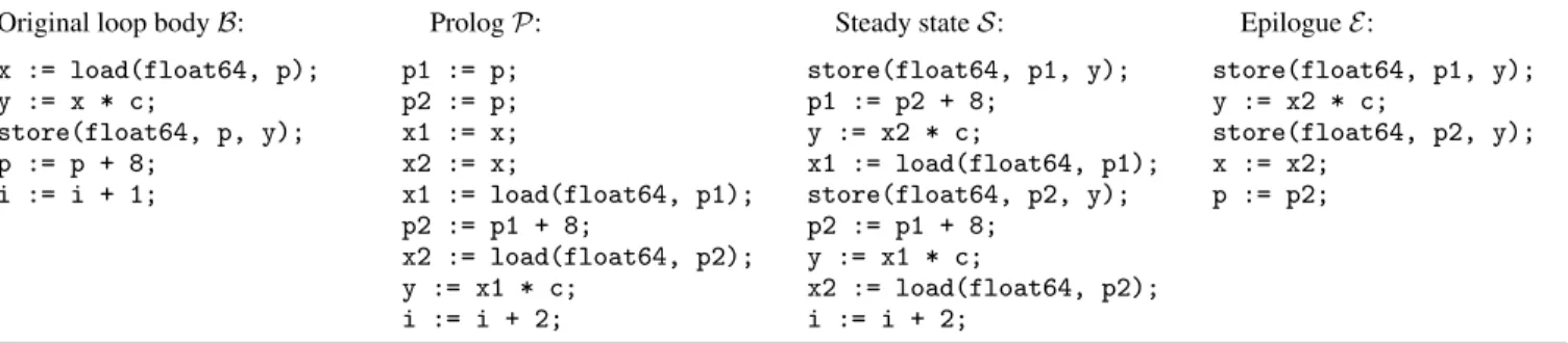
Original loop bodyB: x := load(float64, p); y := x * c; store(float64, p, y); p := p + 8; i := i + 1; PrologP: p1 := p; p2 := p; x1 := x; x2 := x; x1 := load(float64, p1); p2 := p1 + 8; x2 := load(float64, p2); y := x1 * c; i := i + 2; Steady stateS: store(float64, p1, y); p1 := p2 + 8; y := x2 * c; x1 := load(float64, p1); store(float64, p2, y); p2 := p1 + 8; y := x1 * c; x2 := load(float64, p2); i := i + 2; EpilogueE: store(float64, p1, y); y := x2 * c; store(float64, p2, y); x := x2; p := p2;
Figure 1. An example of software pipelining
proof was mechanized using the Coq proof assistant), and infor-mally argued to be complete with respect to a wide class of soft-ware pipelining optimizations.
The formal verification of a validator consists in mechanically proving that if it returns true, its two input programs do behave identically at run time. This is a worthwhile endeavor for two rea-sons. First, it brings additional confidence that the results of vali-dation are trustworthy. Second, it provides an attractive alternative to formally verifying the soundness of the optimization algorithm itself: the validator is often smaller and easier to verify than the op-timization it validates [26]. The validation algorithm presented in this paper grew out of the desire to add a software pipelining pass to the CompCert high-assurance C compiler [11]. Its formal veri-fication in Coq is not entirely complete at the time of this writing, but appears within reach given the simplicity of the algorithm.
The remainder of this paper is organized as follows. Section 2 recalls the effect of software pipelining on the shape of loops. Sec-tion 3 outlines the basic principle of our validator. SecSec-tion 4 defines the flavor of symbolic evaluation that it uses. Section 5 presents the validation algorithm. Its soundness is proved in section 6; its com-pleteness is discussed in section 7. The experience gained on a pro-totype implementation is discussed in section 8. Section 9 discusses related work, and is followed by conclusions and perspectives in section 10.
2.
Software pipelining
From the bird’s eye, software pipelining is performed in three steps. Step 1 Select one inner loop for pipelining. Like in most previous work, we restrict ourselves to simple counted loops of the form
i := 0;
while (i < N ) { B }
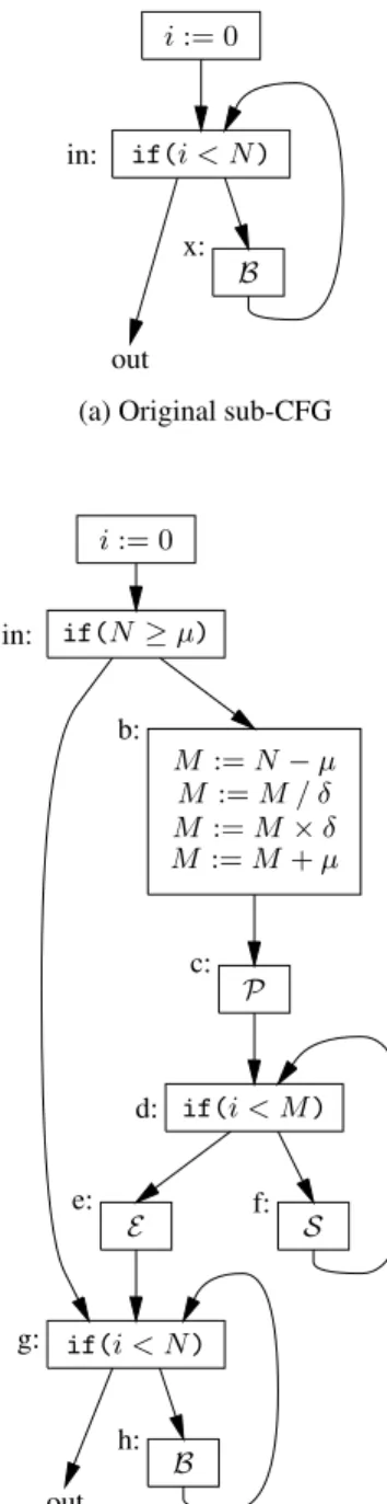
We assume that the loop bound N is a loop-invariant variable, that the loop bodyB is a basic block (no conditional branches, no function calls), and that the loop indexi is incremented exactly once in B. The use of structured control above is a notational convenience: in reality, software pipelining is performed on a flow graph representation of control (CFG), and step 1 actually isolates a sub-graph of the CFG comprising a proper loop of the form above, as depicted in figure 2(a).
Step 2 Next, the software pipeliner is called. It takes as in-put the loop body B and the loop index i, and produces a 5-tuple (P, S, E, µ, δ) as result. P, S and E are sequences of non-branching instructions;µ and δ are positive integers.
•S is the new loop body, also called the steady state of the
pipeline.
•P is the loop prolog: a sequence of instructions that fills the
pipeline until it reaches the steady state.
• E is the loop epilog: a sequence of instructions that drains the
pipeline, finishing the computations that are still in progress at the end of the steady state.
• µ is the minimum number of iterations that must be performed to be able to use the pipelined loop.
• δ is the amount of unrolling that has been performed on the steady state. In other words, one iteration ofS corresponds to δ iterations of the original loopB.
The prologP is assumed to increment the loop index i by µ; the steady stateS, by δ; and the epilogue E, not at all.
The software pipelining algorithms that we have in mind here are combinations of modulo scheduling [22, 7, 15, 23, 4] fol-lowed by modulo variable expansion [10]. However, the presenta-tion above seems general enough to accommodate other scheduling algorithms.
Figure 1 illustrates one run of a software pipeliner. The schedule obtained by modulo scheduling performs, at each iteration, theith store and increment of p, the(i + 1)thmultiplication by c, and the (i + 2)thload. To avoid read-after-write hazards, modulo variable expansion was performed, unrolling the schedule by a factor of 2, and replacing variables p and x by two variables each, p1/p2 and x1/x2, which are defined in an alternating manner. These pairs of variables are initialized from p and x in the prolog; the epilogue sets p and x back to their final values. The unrolling factorδ is therefore 2. Likewise, the minimum number of iterations isµ = 2. Step 3 Finally, the original loop is replaced by the following pseudo-code: i := 0; if (N ≥ µ) { M := ((N − µ)/δ) × δ + µ; P while (i < M ) { S } E } while (i < N ) { B }
In CFG terms, this amounts to replacing the sub-graph shown at the top of figure 2 by the one shown at the bottom.
The effect of the code after pipelining is as follows. If the number of iterationsN is less than µ, a copy of the original loop is executed. Otherwise, we execute the prologP, then iterate the steady stateS, then execute the epilogue E, and finally fall through the copy of the original loop. SinceP and S morally correspond to µ and δ iterations of the original loop, respectively, S is iterated n times wheren is the largest integer such that µ + nδ ≤ N , namely n = (N − µ)/δ. In terms of the loop index i, this corresponds to the upper limitM shown in the pseudo-code above. The copy of the original loop executes the remainingN − M iterations.
i := 0 if(i < N ) B in: out x:
(a) Original sub-CFG
i := 0 if(N ≥ µ) M := N − µ M := M / δ M := M × δ M := M + µ P if(i < M ) S E if(i < N ) B in: out b: c: d: f: e: g: h:
(b) Replacement sub-CFG after software pipelining Figure 2. The effect of software pipelining on a control-flow graph
Steps 1, 2 and 3 can of course be repeated once per inner loop eligible for pipelining. In the remainder of this paper, we focus on the transformation of a single loop.
3.
Validation a posteriori
In a pure translation validation approach, the validator would re-ceive as inputs the code before and after software pipelining and would be responsible for establishing the correctness of all three steps of pipelining. We found it easier to concentrate translation validation on step 2 only (the construction of the components of the pipelined loop) and revert to traditional compiler verification for steps 1 and 3 (the assembling of these components to form the transformed code). In other words, the validator we set out to build
takes as arguments the input(i, N, B) and output (P, S, E, µ, δ) of the software pipeliner (step 2). It is responsible for establishing conditions sufficient to prove semantic preservation between the original and transformed codes (top and bottom parts of figure 2).
What are these sufficient conditions and how can a validator establish them? To progress towards an answer, think of complete unrollings of the original and pipelined loops. We see that the run-time behavior of the original loop is equivalent to that ofBN, that
is,N copies of B executed in sequence. Likewise, the generated code behaves either likeBN
ifN < µ, or like P; Sκ(N ); E; Bρ(N )
ifN ≥ µ, where
κ(N ) def= (N − µ)/δ ρ(N ) def= N − µ − δ × κ(N )
The verification problem therefore reduces to establishing that, for allN , the two basic blocks
XN def= BN and YN def= P; Sκ(N ); E; Bρ(N )
are semantically equivalent: if both blocks are executed from the same initial state (same memory state, same values for variables), they terminate with the same final state (up to the values of tempo-rary variables introduced during scheduling and unused later).
For a given value ofN , symbolic evaluation provides a simple, effective way to ensure this semantic equivalence betweenXN
andYN. In a nutshell, symbolic evaluation is a form of denotational
semantics for basic blocks where the values of variablesx, y, . . . at the end of the block are determined as symbolic expressions of their valuesx0, y0, . . . at the beginning of the block. For example,
the symbolic evaluation of the blockB def= y := x+1; x := y×2 is α(B) = 8 < : x 7→ (x0+ 1) × 2 y 7→ x0+ 1 v 7→ v0for allv /∈ {x, y}
(This is a simplified presentation of symbolic evaluation; section 4 explains how to extend it to handle memory accesses, potential run-time errors, and the fresh variables introduced by modulo variable expansion during pipelining.)
The fundamental property of symbolic evaluation is that if two blocks have identical symbolic evaluations, whenever they are ex-ecuted in the same but arbitrary initial state, they terminate in the same final state. Moreover, symbolic evaluation is insensitive to reordering of independent instructions, making it highly suitable to reason over scheduling optimizations [26]. Therefore, for any givenN , our validator can check that α(XN) = α(YN); this
suf-fices to guarantee thatXNandYNare semantically equivalent.
IfN were a compile-time constant, this would provide us with a validation algorithm. However,N is in general a run-time quan-tity, and statically checkingα(XN) = α(YN) for all N is not
decidable. The key discovery of this paper is that this undecidable property∀N, α(XN) = α(YN) is implied by (and, in practice,
equivalent to) the following two decidable conditions:
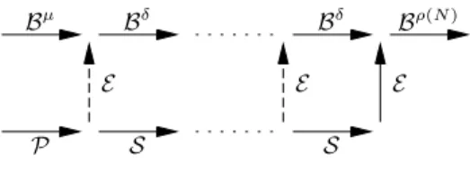
α(E; Bδ) = α(S; E) (1) α(Bµ) = α(P; E) (2) The programmer’s intuition behind condition 1 is the following: in a correct software pipeline, if enough iterations remain to be performed, it should always be possible to choose between 1) execute the steady stateS one more time, then leave the pipelined loop and executeE; or 2) leave the pipelined loop immediately by executingE, then run δ iterations of the original loop body B. (See figure 3.) Condition 2 is even easier to justify: if the number
Bµ Bδ Bδ Bρ(N ) P S S E E E
Figure 3. A view of an execution of the loop, before (top) and after (bottom) pipelining. The dashed vertical arrows provide intuitions for equations 1 and 2.
of executions is exactlyµ, the original code performs Bµ
and the pipelined code performsP; E.
The translation validation algorithm that we define in section 5 is based on checking minor variations of conditions 1 and 2, along with some additional conditions on the evolutions of variable i (also checked using symbolic evaluation). Before presenting this algorithm, proving that it is sound, and arguing that it is complete in practice, we first need to define symbolic evaluation more precisely and study its algebraic structure.
4.
Symbolic evaluation with observables
In this section, we formally define the form of symbolic evaluation used in our validator. Similar forms of symbolic evaluation are at the core of several other translation validators, such as those of Necula [18], Rival [24], and Tristan and Leroy [26].
4.1 The intermediate language
We perform symbolic evaluation over the following simple lan-guage of basic blocks:
Non-branching instructions: I ::= r := r′
variable-variable move | r := op(op, ~r) arithmetic operation | r := load(κ, raddr) memory load
| store(κ, raddr, rval) memory store
Basic blocks:
B ::= I1; . . . ; In instruction sequences
Here,r ranges over variable names (a.k.a. pseudo-registers or tem-poraries); op ranges over arithmetic operators (such as “load inte-ger constantn” or “add integer immediate n” or “float multiply”); andκ stands for a memory quantity (such as “8-bit signed integer” or “64-bit float”).
4.2 Symbolic states
The symbolic evaluation of a block produces a pair(ϕ, σ) of a mapping ϕ from resources to terms, capturing the relationship between the initial and final values of resources, and a set of termsσ, recording the computations performed by the block. Resources:
ρ ::= r | Mem Terms:
t ::= ρ0 initial value ofρ
| Op(op, ~t) result of an operation | Load(κ, taddr, tm) result of a load
| Store(κ, taddr, tval, tm) effect of a store
Resource maps: ϕ ::= ρ 7→ t finite map Computations performed: σ ::= {t1; . . . ; tn} finite set Symbolic states: A ::= (ϕ, σ)
Resource maps symbolically track the values of variables and the memory state, represented like a ghost variable Mem. A resourceρ that is not in the domain of a mapϕ is considered mapped to ρ0.
Memory states are represented by termstmbuilt out of Mem0 and
Store(. . .) constructors. For example, the following block store(κ, x, y); z := load(κ, w) symbolically evaluates to the following resource map:
Mem7→ Store(κ, x0, y0, Mem0)
z 7→ Load(κ, w0, Store(κ, x0, y0, Mem0))
Resource maps describe the final state after execution of a basic block, but do not capture all intermediate operations performed. This is insufficient if some intermediate operations can fail at run-time (e.g.integer divisions by zero or loads from a null pointer). Consider for example the two blocks
y := x and y := load(int32, x); y := x
They have the same resource map, namelyy 7→ x0, yet the
right-most block right can cause a run-time error if the pointerx is null, while the leftmost block never fails. Therefore, resource maps do not suffice to check that two blocks have the same semantics; they must be complemented by setsσ of symbolic terms, recording all the computations that are performed by the blocks, even if these computations do not contribute directly to the final state. Continu-ing the example above, the leftmost block hasσ = ∅ (a move is not considered as a computation, since it cannot fail) while the right-most block hasσ′
= {Load(int32, x0, Mem0)}. Since these two
sets differ, symbolic evaluation reveals that the two blocks above are not semantically equivalent with respect to run-time errors. 4.3 Composition
A resource map ϕ can be viewed as a parallel substitution of symbolic terms for resources: the action of a map on a termt is the termϕ(t) obtained by replacing all occurrences of ρ0 int by
the term associated withρ in ϕ. Therefore, the reverse composition ϕ1; ϕ2of two maps is, classically,
ϕ1; ϕ2 def= {ρ 7→ ϕ1(ϕ2(ρ)) | ρ ∈ Dom(ϕ1) ∪ Dom(ϕ2)} (3)
The reverse composition operator extends naturally to abstract states:
(ϕ1, σ1); (ϕ2, σ2) def= (ϕ1; ϕ2, σ1∪ {ϕ1(t) | t ∈ σ2}) (4)
Composition is associative and admits the identity abstract state ε def= (∅, ∅) as neutral element.
4.4 Performing symbolic evaluation
The symbolic evaluationα(I) of a single instruction I is the ab-stract state defined by
α(r := r′) = (r 7→ r′0, ∅) α(r := op(op, ~r)) = (r 7→ t, {t}) wheret = Op(op, ~r0) α(r := load(κ, r′ )) = (r 7→ t, {t}) wheret = Load(κ, r′ 0, Mem0) α(store(κ, r, r′)) = (Mem 7→ tm, {tm}) wheretm= Store(κ, r0, r ′ 0, Mem0)
Symbolic evaluation then extends to basic blocks, by composing the evaluations of individual instructions:
α(I1; . . . ; In) def
= α(I1); . . . ; α(In) (5)
By associativity, it follows that symbolic evaluation distributes over concatenation of basic blocks:
α(B1; B2) = α(B1); α(B2) (6)
4.5 Comparing symbolic states
We use two notions of equivalence between symbolic states. The first one, written∼, is defined as strict syntactic equality:2
(ϕ, σ) ∼ (ϕ′
, σ′
) if and only if ∀ρ, ϕ(ρ) = ϕ′
(ρ) and σ = σ′
(7) The relation∼ is therefore an equivalence relation, and is compat-ible with composition:
A1∼ A2=⇒ A1; A ∼ A2; A (8)
A1∼ A2=⇒ A; A1∼ A; A2 (9)
We need a coarser equivalence between symbolic states to ac-count for the differences in variable usage between the code before and after software pipelining. Recall that pipelining may perform modulo variable expansion to avoid read-after-write hazards. This introduces fresh temporary variables in the pipelined code. These fresh variables show up in symbolic evaluations and prevent strict equivalence∼ from holding. Consider:
x := op(op, x) and x′
:= op(op, x) x := x′
These two blocks have different symbolic evaluations (in the sense of the∼ equivalence), yet should be considered as semantically equivalent if the temporaryx′
is unused later.
Letθ be a finite set of variables: the observable variables. (In our validation algorithm, we takeθ to be the set of all variable mentioned in the original code before pipelining; the fresh tem-poraries introduced by modulo variable expansion are therefore not inθ.) Equivalence between symbolic states up to the observables θ is written≈θand defined as
(ϕ, σ) ≈θ(ϕ ′
, σ′) if and only if
∀ρ ∈ θ ∪ {Mem}, ϕ(ρ) = ϕ′(ρ) and σ = σ′ (10) The relation ≈θ is an equivalence relation, coarser than ∼, and
compatible with composition on the right:
A1∼ A2=⇒ A1≈θA2 (11)
A1≈θA2=⇒ A; A1≈θ A; A2 (12)
However, it is not, in general, compatible with composition on the left. Consider an abstract stateA that maps a variable x ∈ θ to a termt containing an occurrence of y /∈ θ. Further assume A1 ≈θ A2. The compositionA1; A maps x to A1(t); likewise,
A2; A maps x to A2(t). Since y /∈ θ, we can have A1(y) 6= A2(y)
and therefore A1(t) 6= A2(t) without violating the hypothesis
A1≈θA2. Hence,A1; A ≈θ A2; A does not hold in general.
To address this issue, we restrict ourselves to symbolic states A that are contained in the set θ of observables. We say that a
2 We could relax this definition in two ways. One is to compare symbolic
terms up to a decidable equational theory capturing algebraic identities such as x × 2 = x + x. This enables the validation of e.g. instruction strength reduction [18, 24]. Another relaxation is to require s′ ⊆ sinstead of s =
s′, enabling the transformed basic block to perform fewer computations than the original block (e.g. dead code elimination). Software pipelining being a purely lexical transformation that changes only the placement of computations but not their nature nor their number, these two relaxations are not essential and we stick with strict syntactic equality for the time being.
Semantic interpretation of arithmetic and memory operations: op : list val→ option val
load : quantity× val × mem → option val store : quantity× val × val × mem → option mem Transition semantics for instructions:
r := r′ : (R, M ) → (R[r ← R(r′ )], M ) op(R(~r)) = ⌊v⌋ r := op(op, ~r) : (R, M ) → (R[r ← v], M ) load(κ, R(raddr), M ) = ⌊v⌋ r := load(κ, raddr) : (R, M ) → (R[r ← v], M )
store(κ, R(raddr), R(rval), M ) = ⌊M′⌋
store(κ, raddr, rval) : (R, M ) → (R, M′)
Transition semantics for basic blocks:
ε : S→ S∗ I : S → S
′
B : S′ ∗
→ S′′
I.B : S→ S∗ ′′
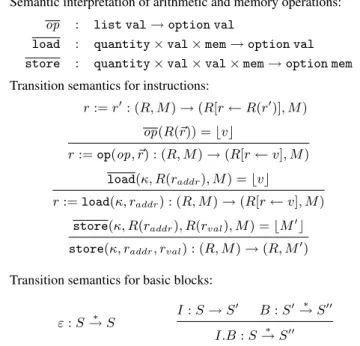
Figure 4. Operational semantics for basic blocks
symbolic termt is contained in θ, and write t ⊑ θ, if all variables x appearing int belong to θ. We extend this notion to symbolic states as follows:
(ϕ, σ) ⊑ θ if and only if
∀ρ ∈ θ ∪ {Mem}, ϕ(ρ) ⊑ θ and ∀t ∈ σ, t ⊑ θ (13) It is easy to see that≈θis compatible with composition on the left
if the right symbolic state is contained inθ:
A1≈θ A2 ∧ A ⊑ θ =⇒ A1; A ≈θA2; A (14)
The containment relation enjoys additional useful properties: A1⊑ θ ∧ A1≈θA2 =⇒ A2⊑ θ (15)
A1⊑ θ ∧ A2⊑ θ =⇒ (A1; A2) ⊑ θ (16)
4.6 Semantic soundness
The fundamental property of symbolic evaluation is that if α(B1) ≈θ α(B2), the two blocks B1 and B2 have the same
run-time behavior, in a sense that we now make precise.
We equip our language of basic blocks with the straightforward operational semantics shown in figure 4. The behavior of arithmetic and memory operations is axiomatized as functions op, load and store that return “option” types to model run-time failures: the result∅ (pronounced “none”) denotes failure; the result ⌊x⌋ (pro-nounced “somex”) denotes success. In our intended application, these interpretation functions are those of the RTL intermediate lan-guage of the CompCert compiler [12, section 6.1] and of its mem-ory model [13].
The semantics for a basic blockB is, then, given as the relation B : S→ S∗ ′
, sometimes also writtenS→ SB ′
, whereS is the initial state andS′
the final state. States are pairs(R, M ) of a variable stateR, mapping variables to values, and a memory state M .
We say that two execution states S = (R, M ) and S′
= (R′
, M′
) are equivalent up to the observables θ, and write S ∼=θ
S′
, ifM = M′
andR(r) = R′(r) for all r ∈ θ.
THEOREM1 (Soundness of symbolic evaluation). LetB1andB2 be two basic blocks. Assume thatα(B1) ≈θ α(B2) and α(B2) ⊑
θ. If B1 : S ∗
→ S′
and S ∼=θ T , there exists T ′ such that B2 : T ∗ → T′ andS′∼ =θ T′.
We omit the proof, which is similar to that of Lemma 3 in [26].
5.
The validation algorithm
We can now piece together the intuitions from section 3 and the definitions from section 4 to obtain the following validation algo-rithm: validate(i, N, B) (P, S, E, µ, δ) θ = α(Bµ) ≈ θα(P; E) (A) ∧ α(E; Bδ) ≈ θ α(S; E) (B) ∧ α(B) ⊑ θ (C) ∧ α(B)(i) = Op(addi(1), i0) (D) ∧ α(P)(i) = α(Bµ)(i) (E) ∧ α(S)(i) = α(Bδ)(i) (F) ∧ α(E)(i) = i0 (G) ∧ α(B)(N ) = α(P)(N ) = α(S)(N ) = α(E)(N ) = N0 (H)
The inputs of the validator are the components of the loops be-fore(i, N, B) and after (P, S, E, µ, δ) pipelining, as well as the set θ of observables. Checks A and B correspond to equations (1) and (2) of section 3, properly reformulated in terms of equiva-lence up to observables. Check C makes sure that the setθ of ob-servables includes at least the variables appearing in the symbolic evaluation of the original loop bodyB. Checks D to G ensure that the loop indexi is incremented the way we expect it to be: by one inB, by µ in P, by δ in S, and not at all in E. (We write α(B)(i) to refer to the symbolic term associated toi by the resource map part of the symbolic stateα(B).) Finally, check H makes sure that the loop limitN is invariant in both loops.
The algorithm above has low computational complexity. Using a hash-consed representation of symbolic terms, the symbolic eval-uationα(B) of a block B containing n instructions can be com-puted in timeO(n log n): for each of the n instructions, the algo-rithm performs one update on the resource map, one insertion in the constraint set, and one hash-consing operation, all of which can be done in logarithmic time. (The resource map and the constraint set have sizes at mostn.) Likewise, the equivalence and containment relations (≈θ and⊑) can be decided in time O(n log n). Finally,
note that thisO(n log n) complexity holds even if the algorithm is implemented within the Coq specification language, using persis-tent, purely functional data structures.
The running time of the validation algorithm is therefore O(n log n) where n = max(µ|B|, δ|B|, |P|, |S|, |E|) is pro-portional to the size of the loop after pipelining. Theoretically, software pipelining can increase the size of the loop quadratically. In practice, we expect the external implementation of software pipelining to avoid this blowup and produce code whose size is linear in that of the original loop. In this case, the validator runs in timeO(n log n) where n is the size of the original loop.
6.
Soundness proof
In this section, we prove the soudness of the validator: if it returns “true”, the software pipelined loop executes exactly like the origi-nal loop. The proof proceeds in two steps: first, we show that the ba-sic blocksXNandYNobtained by unrolling the two loops have the
same symbolic evaluation and therefore execute identically; then, we prove that the concrete execution of the two loops in the CFG match.
6.1 Soundness with respect to the unrolled loops
We first show that the finitary conditions checked by the validator imply the infinitary equivalences between the symbolic evaluations ofXNandYNsketched in section 3.
LEMMA2. If validate(i, N, B) (P, S, E, µ, δ) θ returns true,
then, for alln,
α(Bµ+nδ) ≈θα(P; Sn; E) (17)
α(P; Sn; E) ⊑ θ (18) α(Bµ+nδ)(i) = α(P; Sn)(i) = α(P; Sn; E)(i)
(19) Proof:By hypothesis, we know that the properties A to H checked by the validator hold. First note that
∀n, α(Bn) ⊑ θ (20) as a consequence of check C and property (16).
Conclusion (17) is proved by induction onn. The base case n = 0 reduces to α(Bµ) ≈
θα(P; E), which is ensured by check A. For
the inductive case, assumeα(Bµ+nδ) ≈
θα(P; Sn; E).
α(Bµ+(n+1)δ) ≈θα(Bµ+nδ); α(Bδ)
(by distributivity (6)) ≈θα(P; Sn; E); α(Bδ)
(by left compatibility (14) and ind. hyp.) ≈θα(P; Sn); α(E; Bδ)
(by distributivity (6)) ≈θα(P; Sn); α(S; E)
(by check B, right compatibility (12), and (20)) ≈θα(P; Sn+1; E)
(by distributivity (6))
Conclusion (18) follows from (17), (20), and property (15). Con-clusion (19) follows from checks E, F and G by induction onn. ✷ THEOREM3. Assume that validate(i, N, B) (P, S, E, µ, δ) θ
returnstrue. Consider an executionBN: S ∗
→ S′
of the unrolled initial loop, withN ≥ µ. Assume S ∼=θ T . Then, there exists a concrete stateT′ such that P; Sκ(N ); E; Bρ(N ): T→ T∗ ′ (21) S′∼ =θT ′ (22)
Moreover, execution (21) decomposes as follows:
T → TP 0 S → · · ·→S | {z } κ(N )times Tκ(N ) E → T′ 0 B → · · ·→B | {z } ρ(N )times Tρ(N )′ = T ′ (23)
and the values of the loop indexi in the various intermediate states
satisfy
Tj(i) = S(i) + µ + δj (mod 232) (24)
T′
j(i) = S(i) + µ + δ × κ(N ) + j (mod 232) (25)
Proof:As a corollary of Lemma 2, properties (17) and (18), we obtain
α(BN) ≈
θα(P; Sκ(N ); E; Bρ(N ))
α(P; Sκ(N ); E; Bρ(N )) ⊑ θ sinceN = µ + δ × κ(N ) + ρ(N ). The existence of T′
then follows from Theorem 1.
It is obvious that the concrete execution of the pipelined code can be decomposed as shown in (23). Check D in the validator
CFG instructions:
Ig::= (I, ℓ) non-branching instr.
| (if(r < r′ ), ℓt, ℓf) conditional branch CFG: g ::= ℓ 7→ Ig finite map Transition semantics: g(ℓ) = (I, ℓ′ ) I : (R, M ) → (R′ , M′ ) (as in figure 4) g : (ℓ, R, M ) → (ℓ′, R′, M′) g(ℓ) = (if(r < r′ ), ℓt, ℓf) ℓ′= ( ℓt ifR(r) < R(r′) ℓf ifR(r) ≥ R(r′) g : (ℓ, R, M ) → (ℓ′ , R, M )
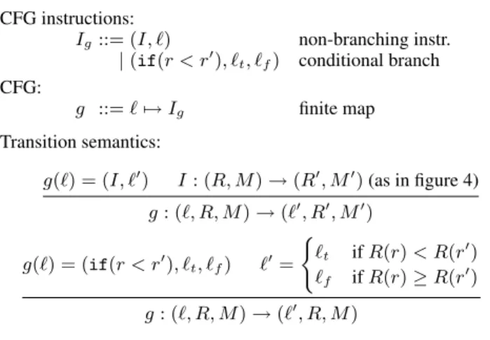
Figure 5. A simple language of control-flow graphs
guarantees thatSj+1(i) = Sj(i) + 1 (mod 232), which implies
Sj(i) = S(i) + j mod 232. Combined with conclusion (19) of
Lemma 2, this implies equation (24):
Tj(i) = Sµ+δj(i) = S(i) + µ + δj (mod 232)
as well as
T0′(i) = Sµ+δ×κ(N )(i) = S(i) + µ + δ × κ(N ) (mod 232)
Check D entails thatT′ j(i) = T
′
0(i) + j mod 232. Equation (25)
therefore follows. ✷
6.2 Soundness with respect to CFG loops
The second and last part of the soundness proof extends the semantic preservation results of theorem 3 from the unrolled loops in a basic-block representation to the actual loops in a CFG (control-flow graph) representation, namely the loops before and after pipelining depicted in figure 2. This extension is intuitively obvious but surprisingly tedious to formalize in full details: indeed, this is the only result in this paper that we have not yet mechanized in Coq.
Our final objective is to perform instruction scheduling on the RTL intermediate language from the CompCert compiler [12, sec-tion 6.1]. To facilitate exposisec-tion, we consider instead the simpler language of control-flow graphs defined in figure 5. The CFG g is represented as partial map from labelsℓ to instructions Ig. An
instruction can be either a non-branching instructionI or a condi-tional branch if(r < r′
), complemented by one or two labels de-noting the successors of the instruction. The operational semantics of this language is given by a transition relationg : (ℓ, R, M ) → (ℓ′
, R′
, M′
) between states comprising a program point ℓ, a regis-ter stateR and a memory state M .
The following trivial lemma connects the semantics of basic blocks (figure 4) with the semantics of CFGs (figure 5). We say that a CFGg contains the basic block B between points ℓ and ℓ′
, and writeg, B : ℓ ❀ ℓ′
, if there exists a path ing from ℓ to ℓ′
that “spells out” the instructionsI1, . . . , InofB:
g(ℓ) = (I1, ℓ1) ∧ g(ℓ1) = (I2, ℓ2) ∧ · · · ∧ g(ℓn) = (In, ℓ ′ ) LEMMA4. Assumeg, B : ℓ ❀ ℓ′ . Then,g : (ℓ, S)→ (ℓ∗ ′ , S′ ) if and only ifB : S→ S∗ ′ .
In the remainder of this section, we consider two control-flow graphs:g for the original loop before pipelining, depicted in part (a) of figure 2, andg′
for the loop after pipelining, depicted in part (b) of figure 2. (Note that figure 2 is not a specific example: it describes
the general shape of CFGs accepted and produced by all software pipelining optimizations we consider in this paper.) We now use lemma 4 to relate a CFG execution of the original loopg with the basic-block execution of its unrolling.
LEMMA5. Assumeα(B)(i) = Op(addi(1), i0) and α(B)(N ) =
N0. Consider an executiong : (in, S) ∗
→ (out, S′
) from point in
to pointout in the original CFG, withS(i) = 0. Then, BN : S ∗
→ S′
whereN is the value of variable N in state S.
Proof:The CFG execution can be decomposed as follows: (in, S0) → (x, S0)
∗
→ (in, S1) → · · · ∗
→ (in, Sn) → (out, Sn)
withS = S0 andS′ = SnandSn(i) ≥ Sn(N ) and Sj(i) <
Sj(N ) for all j < n. By construction of B, we have g, B : x ❀ in.
Therefore, by Lemma 4,B : Sj ∗
→ Sj+1forj = 0, . . . , n − 1.
It follows thatBn : S ∗
→ S′
. Moreover, at each loop iteration, variableN is unchanged and variable i is incremented by 1. It follows that the numbern of iterations is equal to the value N of variableN in initial state S. This is the expected result. ✷ Symmetrically, we can reconstruct a CFG execution of the pipelined loopg′
from the basic-block execution of its unrolling. LEMMA6. LetTinitbe an initial state where variablei has value
0 and variable N has value N . Let T be Tinitwhere variableM is set toµ + δ × κ(N ). Assume that properties (23), (24) and (25)
hold, as well as check H. We can, then, construct an execution
g′
: (in, Tinit) ∗
→ (out, T′
) from point in to point out in the
CFGg′ after pipelining. Proof:By construction ofg′ , we haveg′ , P : c ❀ d and g′ , S : f ❀ d and g′, E : e ❀ g and g′ , B : h ❀ g. The result is obvious ifN < µ. Otherwise, applying Lemma 4 to the basic-block executions given by property (23), we obtain the following CFG executions: g′ : (in, Tinit) ∗ → (c, T ) g′ : (c, T )→ (d, T∗ 0) g′ : (f, Tj) ∗ → (d, Tj+1) for j = 0, . . . , κ(N ) − 1 g′: (e, Tκ(N )) ∗ → (g, T′ 0) g′: (h, Tj′) ∗ → (g, T′ j+1) for j = 0, . . . , ρ(N ) − 1
The variablesN and M are invariant between points c and out: N because of check H, M because it is a fresh variable. Using properties (24) and (25), we see that the condition at point d is true in statesT0, . . . , Tκ(N )−1 and false in stateTκ(N ). Likewise, the
condition at point g is true in statesT′
0, . . . , Tρ(N )−1′ and false in
stateT′
ρ(N ). The expected result follows. ✷
Piecing everything together, we obtain the desired semantic preservation result.
THEOREM7. Assume that validate(i, N, B) (P, S, E, µ, δ) θ
returnstrue. Letg and g′
be the CFG before and after pipelining, respectively. Consider an executiong : (in, S)→ (out, S∗ ′
) with S(i) = 0. Then, for all states T such that S ∼=θ T , there exists a stateT′ such thatg′ : (in, T )→ (out, T∗ ′ ) and S′∼ =θT ′ .
Proof:Follows from Theorem 3 and Lemmas 5 and 6. ✷
7.
Discussion of completeness
Soundness (rejecting all incorrect code transformations) is the fun-damental property of a validator; but relative completeness (not re-jecting valid code transformations) is important in practice, since
a validator that reports many false positives is useless. Seman-tic equivalence between two arbitrary pieces of code being unde-cidable, a general-purpose validation algorithm cannot be sound and complete at the same time. However, a specialized valida-tor can still be sound and complete for a specific class of pro-gram transformations—in our case, software pipelining optimiza-tions based on modulo scheduling and modulo variable expansion. In this section, we informally discuss the sources of potential in-completeness for our validator.
Mismatch between infinitary and finitary symbolic evaluation A first source of potential incompleteness is the reduction of the infinitary condition ∀N, α(XN) = α(YN) to the two finitary
checks A and B. More precisely, the soundness proof of section 6 hinges on the following implication being true:
(A) ∧ (B) =⇒ (17) or in other words,
α(Bµ) ≈θα(P; E) ∧ α(E; Bδ) ≈θα(S; E)
=⇒ ∀n, α(Bµ+nδ) ≈θ α(P; Sn; E)
However, the reverse implication does not hold in general. Assume that (17) holds. Takingn = 0, we obtain equation (A). However, we cannot prove (B). Exploiting (17) forn and n + 1 iterations, we obtain:
α(Bµ+nδ) ≈θα(P; Sn); α(E)
α(Bµ+nδ); α(Bδ) ≈θα(P; Sn); α(S; E)
Combining these two equivalences, it follows that
α(P; Sn); α(E; Bδ) ≈θα(P; Sn); α(S; E) (26)
However, we cannot just “simplify on the left” and conclude α(E; Bδ) ≈
θ α(S; E). To see why such simplifications are
incorrect, consider the two blocks
x := 1; and x := 1; y := 1 y := x
We haveα(x := 1); α(y := 1) ≈θ α(x := 1); α(y := x) with
θ = {x, y}. However, the equivalence α(y := 1) ≈θ α(y := x)
does not hold.
Coming back to equation (26), the blocksE; Bδ
andS; E could make use of some property of the state set up byP; Sn
(such as the fact thatx = 1 in the simplified example above). However, (26) holds for any numbern of iteration. Therefore, this hypothetical property of the state that invalidates (B) must be a loop invariant. We are not aware of any software pipelining algorithm that takes advantage of loop invariants such as x = 1 in the simplified example above.
In conclusion, the reverse implication(17) =⇒ (A) ∧ (B), which is necessary for completeness, is not true in general, but we strongly believe it holds in practice as long as the software pipelining algorithm used is purely syntactic and does not exploit loop invariants.
Mismatch between symbolic evaluation and concrete executions A second, more serious source of incompleteness is the following: equivalence between the symbolic evaluations of two basic blocks is a sufficient, but not necessary condition for those two blocks to execute identically. Here are some counter-examples.
1. The two blocks could execute identically because of some prop-erty of the initial state, as in
y := 1 vs. y := x assumingx = 1 initially.
2. Symbolic evaluation fails to account for some algebraic proper-ties of arithmetic operators:
i := i + 1; vs. i := i + 2 i := i + 1
3. Symbolic evaluation fails to account for memory separation properties within the same memory block:
store(int32, p + 4, y); vs. x := load(int32, p); x := load(int32, p) store(int32, p + 4, y) 4. Symbolic evaluation fails to account for memory separation
properties within different memory blocks:
store(int32, a, y); vs. x := load(int32, b); x := load(int32, b) store(int32, a, y) assuming thata and b point to different arrays.
Mismatches caused by specific properties of the initial state, as in example 1 above, are not a concern for us: as previously argued, it is unlikely that the pipelining algorithm would take advantage of these properties. The other three examples are more problem-atic: software pipeliners do perform some algebraic simplifications (mostly, on additions occurring within address computations and loop index updates) and do take advantage of nonaliasing proper-ties to hoist loads above stores.
Symbolic evaluation can be enhanced in two ways to address these issues. The first way, pioneered by Necula [18], consists in comparing symbolic terms and states modulo an equational theory capturing the algebraic identities and “good variable” properties of interest. For example, the following equational theory addresses the issues illustrated in examples 2 and 3:
Op(addi(n), Op(addi(m), t)) ≡ Op(addi(n + m), t) Load(κ′
, t1, Store(κ, t2, tv, tm)) ≡ Load(κ′, t2, tm)
if|t2− t1| ≥ sizeof(κ)
The separation condition between the symbolic addressest1 and
t2can be statically approximated using a decision procedure such
as Pugh’s Omega test [21]. In practice, a coarse approximation, restricted to the case wheret1 and t2 differ by a compile-time
constant, should work well for software pipelining.
A different extension of symbolic evaluation is needed to ac-count for nonaliasing properties between separate arrays or mem-ory blocks, as in example 4. Assume that these nonaliasing prop-erties are represented by region annotations on load and store in-structions. We can, then, replace the single resource Mem that sym-bolically represent the memory state by a family of resources Memx
indexed by region identifiersx. A load or store in region x is, then, symbolically evaluated in terms of the resource Memx. Continuing
example 4 above and assuming that the store takes place in regiona and the load in regionb, both blocks symbolically evaluate to
Mema7→ Store(int32, a0, y0, Mema0)
x 7→ Load(int32, b0, Memb0)
8.
Implementation and preliminary experiments
The first author implemented the validation algorithm presented here as well as a reference software pipeliner. Both components are implemented in OCaml and were connected with the CompCert C compiler for testing.
The software pipeliner accounts for approximately 2000 lines of OCaml code. It uses a backtracking iterative modulo scheduler [2, chapter 20] to produce a steady state. Modulo variable expan-sion is then performed following Lam’s approach [10]. The mod-ulo scheduler uses a heuristic function to decide the order in which
Figure 6. The symbolic values assigned to register 50 (left) and to its pipelined counterpart, register 114 (right). The pipelined value lacks one iteration due to a corner case error in the implementation of the modulo variable expansion. Symbolic evaluation was performed by omitting the prolog and epilog moves, thus showing the difference in register use.
to consider the instructions for scheduling. We tested our software pipeliner with two such heuristics. The first one randomly picks the nodes. We use it principally to stress the pipeliner and the valida-tor. The second one picks the node using classical dependencies constraints. We also made a few schedules by hand.
We experimented our pipeliner on the CompCert benchmark suite, which contains, among others, some numerical kernels such as a fast Fourier transform. On these examples, the pipeliner performs significant code rearrangements, although the observed speedups are modest. There are several reasons for this: we do not exploit the results of an alias analysis; our heuristics are not state of the art; and we ran our programs on an out-of-order PowerPC G5 processor, while software pipelining is most effective on in-order processors.
The implementation of the validator follows very closely the al-gorithm presented in this paper. It accounts for approximately 300 lines of OCaml code. The validator is instrumented to produce a lot of debug information, including in the form of drawings of sym-bolic states. The validator found many bugs during the develop-ment of the software pipeliner, especially in the impledevelop-mentation of modulo variable expansion. The debugging information produced by the validator was an invaluable tool to understand and correct these mistakes. Figure 6 shows the diagrams produced by our val-idator for one of these bugs. We would have been unable to get the pipeliner right without the help of the validator.
On our experiments, the validator reported no false alarms. The running time of the validator is negligible compared with that of the software pipeliner itself (less than 5%). However, our software pipeliner is not state-of-the-art concerning the determination of the minimal initiation interval, and therefore is relatively costly in terms of compilation time.
Concerning formal verification, the underlying theory of sym-bolic evaluation (section 4) and the soundness proof with respect to unrolled loops (section 6.1) were mechanized using the Coq proof assistant. The Coq proof is not small (approximately 3500 lines) but is relatively straightforward: the mechanization raised no un-expected difficulties. The only part of the soundness proof that we have not mechanized yet is the equivalence between unrolled loops and their CFG representations (section 6.2): for such an intuitively obvious result, a mechanized proof is infuriatingly difficult. Simply proving that the situation depicted in figure 2(a) holds (we have a proper, counted loop whose body is the basic blockB) takes a great deal of bureaucratic formalization. We suspect that the CFG repre-sentation is not appropriate for this kind of proofs; see section 10 for a discussion.
9.
Related work
This work is not the first attempt to validate software pipelining a
posteriori. Leviathan and Pnueli [14] present a validator for a soft-ware pipeliner for the IA-64 architecture. The pipeliner makes use of a rotating register file and predicate registers, but from a valida-tion point of view it is almost the same problem as the one studied in this paper. Using symbolic evaluation, the validator generates a set of verification conditions that are discharged by a theorem prover. We chose to go further with symbolic evaluation: instead of using it to generate verification conditions, we use it to directly establish semantic preservation. We believe that the resulting val-idator is simpler and algorithmically more efficient. However, ex-ploiting nonaliasing information during validation could possibly be easier in Leviathan and Pnueli’s approach than in our approach. Another attempt at validating software pipelining is the one of Kundu et al. [9]. It proceeds by parametrized translation valida-tion. The software pipelining algorithm they consider is based on code motion, a rarely-used approach very different from the mod-ulo scheduling algorithms we consider. This change of algorithms makes the validation problem rather different. In the case of Kundu
et al., the software pipeliner proceeds by repeated rewriting of the original loop, with each rewriting step being validated. In contrast, modulo scheduling builds a pipelined loop in one shot (usually us-ing a backtrackus-ing algorithm). It could possibly be viewed as a se-quence of rewrites but this would be less efficient than our solution. Another approach to establishing trust in software pipelining is run-time validation, as proposed by Goldberg et al. [5]. Their approach takes advantages of the IA-64 architecture to instrument the pipelined loop with run-time check that verify properties of the pipelined loop and recover from unexpected problems. This tech-nique was used to verify that aliasing is not violated by instruction switching, but they did not verify full semantic preservation.
10.
Conclusions
Software pipelining is one of the pinnacles of compiler optimiza-tions; yet, its semantic correctness boils down to two simple se-mantic equivalence properties between basic blocks. Building on this novel insight, we presented a validation algorithm that is simple enough to be used as a debugging tool when implementing software pipelining, efficient enough to be integrated in production compil-ers and executed at every compilation run, and mathematically ele-gant enough to lend itself to formal verification.
Despite its respectable age, symbolic evaluation—the key tech-nique behind our validator—finds here an unexpected application
to the verification of a loop transformation. Several known exten-sions of symbolic evaluation can be integrated to enhance the preci-sion of the validator. One, discussed in section 7, is the addition of an equational theory and of region annotations to take nonaliasing information into account. Another extension would be to perform symbolic evaluation over extended basic blocks (acyclic regions of the CFG) instead of basic blocks, like Rival [24] and Tristan and Leroy [26] do. This extension could make it possible to validate pipelined loops that contain predicated instructions or even condi-tional branches.
From a formal verification standpoint, symbolic evaluation lends itself well to mechanization and gives a pleasant denotational flavor to proofs of semantic equivalence. This stands in sharp contrast with the last step of our proof (section 6.2), where the low-level operational nature of CFG semantics comes back to haunt us. We are led to suspect that control-flow graphs are a poor representation to reason over loop transformations, and to wish for an alternate representation that would abstract the syntactic details of loops just as symbolic evaluation abstracts the syntactic details of (extended) basic blocks. Two promising candidates are the PEG representation of Tate et al. [25] and the representation as sets of mutually recursive HOL functions of Myreen and Gordon [17]. It would be interesting to reformulate software pipelining validation in terms of these representations.
Acknowledgments
This work was supported by Agence Nationale de la Recherche, project U3CAT, program ANR-09-ARPEGE. We thank Franc¸ois Pottier, Alexandre Pilkiewicz, and the anonymous reviewers for their careful reading and suggestions for improvements.
References
[1] A. V. Aho, M. Lam, R. Sethi, and J. D. Ullman. Compilers: principles,
techniques, and tools. Addison-Wesley, second edition, 2006. [2] A. W. Appel. Modern Compiler Implementation in ML. Cambridge
University Press, 1998.
[3] C. W. Barret, Y. Fang, B. Goldberg, Y. Hu, A. Pnueli, and L. Zuck. TVOC: A translation validator for optimizing compilers. In Computer
Aided Verification, 17th Int. Conf., CAV 2005, volume 3576 of LNCS, pages 291–295. Springer, 2005.
[4] J. M. Codina, J. Llosa, and A. Gonz´alez. A comparative study of modulo scheduling techniques. In Proc. of the 16th international
conference on Supercomputing, pages 97–106. ACM, 2002. [5] B. Goldberg, E. Chapman, C. Huneycutt, and K. Palem. Software
bubbles: Using predication to compensate for aliasing in software pipelines. In 2002 International Conference on Parallel Architectures
and Compilation Techniques (PACT 2002), pages 211–221. IEEE Computer Society Press, 2002.
[6] Y. Huang, B. R. Childers, and M. L. Soffa. Catching and identifying bugs in register allocation. In Static Analysis, 13th Int. Symp., SAS
2006, volume 4134 of LNCS, pages 281–300. Springer, 2006. [7] R. A. Huff. Lifetime-sensitive modulo scheduling. In Proc. of the
ACM SIGPLAN ’93 Conf. on Programming Language Design and Implementation, pages 258–267. ACM, 1993.
[8] A. Kanade, A. Sanyal, and U. Khedker. A PVS based framework for validating compiler optimizations. In SEFM ’06: Proceedings of the
Fourth IEEE International Conference on Software Engineering and Formal Methods, pages 108–117. IEEE Computer Society, 2006. [9] S. Kundu, Z. Tatlock, and S. Lerner. Proving optimizations correct
using parameterized program equivalence. In Proceedings of the 2009
Conference on Programming Language Design and Implementation (PLDI 2009), pages 327–337. ACM Press, 2009.
[10] M. Lam. Software pipelining: An effective scheduling technique for VLIW machines. In Proc. of the ACM SIGPLAN ’88 Conf. on
Programming Language Design and Implementation, pages 318–328. ACM, 1988.
[11] X. Leroy. Formal verification of a realistic compiler. Commun. ACM, 52(7):107–115, 2009.
[12] X. Leroy. A formally verified compiler back-end. Journal of
Automated Reasoning, 2009. To appear.
[13] X. Leroy and S. Blazy. Formal verification of a C-like memory model and its uses for verifying program transformations. Journal of
Automated Reasoning, 41(1):1–31, 2008.
[14] R. Leviathan and A. Pnueli. Validating software pipelining optimizations. In Int. Conf. on Compilers, Architecture, and Synthesis
for Embedded Systems (CASES 2002), pages 280–287. ACM Press, 2006.
[15] J. Llosa, A. Gonz´alez, E. Ayguad´e, and M. Valero. Swing modulo scheduling: A lifetime-sensitive approach. In IFIP WG10.3 Working
Conference on Parallel Architectures and Compilation Techniques, pages 80–86, 1996.
[16] S. S. Muchnick. Advanced compiler design and implementation. Morgan Kaufmann, 1997.
[17] M. O. Myreen and M. J. C. Gordon. Transforming programs into recursive functions. In Brazilian Symposium on Formal Methods
(SBMF 2008), volume 240 of ENTCS, pages 185–200. Elsevier, 2009.
[18] G. C. Necula. Translation validation for an optimizing compiler. In Programming Language Design and Implementation 2000, pages 83–95. ACM Press, 2000.
[19] A. Pnueli, O. Shtrichman, and M. Siegel. The code validation tool (CVT) – automatic verification of a compilation process.
International Journal on Software Tools for Technology Transfer, 2(2):192–201, 1998.
[20] A. Pnueli, M. Siegel, and E. Singerman. Translation validation. In Tools and Algorithms for Construction and Analysis of Systems,
TACAS ’98, volume 1384 of LNCS, pages 151–166. Springer, 1998. [21] W. Pugh. The Omega test: a fast and practical integer programming
algorithm for dependence analysis. In Supercomputing ’91:
Proceedings of the 1991 ACM/IEEE conference on Supercomputing, pages 4–13. ACM Press, 1991.
[22] B. R. Rau. Iterative modulo scheduling. International Journal of
Parallel Processing, 24(1):1–102, 1996.
[23] B. R. Rau, M. S. Schlansker, and P. P. Timmalai. Code generation schema for modulo scheduled loops. Technical Report HPL-92-47, Hewlett-Packard, 1992.
[24] X. Rival. Symbolic transfer function-based approaches to certified compilation. In 31st symposium Principles of Programming
Languages, pages 1–13. ACM Press, 2004.
[25] R. Tate, M. Stepp, Z. Tatlock, and S. Lerner. Equality saturation: a new approach to optimization. In 36th symposium Principles of
Programming Languages, pages 264–276. ACM Press, 2009. [26] J.-B. Tristan and X. Leroy. Formal verification of translation
validators: A case study on instruction scheduling optimizations. In 35th symposium Principles of Programming Languages, pages 17–27. ACM Press, 2008.
[27] J.-B. Tristan and X. Leroy. Verified validation of Lazy Code Motion. In Proceedings of the 2009 Conference on Programming Language
Design and Implementation (PLDI 2009), pages 316–326. ACM Press, 2009.
[28] L. Zuck, A. Pnueli, Y. Fang, and B. Goldberg. VOC: A methodology for translation validation of optimizing compilers. Journal of Universal Computer Science, 9(3):223–247, 2003.
[29] L. Zuck, A. Pnueli, and R. Leviathan. Validation of optimizing compilers. Technical Report MCS01-12, Weizmann institute of Science, 2001.