HAL Id: hal-00511224
https://hal.archives-ouvertes.fr/hal-00511224
Submitted on 5 Jul 2011
HAL is a multi-disciplinary open access
archive for the deposit and dissemination of
sci-entific research documents, whether they are
pub-lished or not. The documents may come from
teaching and research institutions in France or
L’archive ouverte pluridisciplinaire HAL, est
destinée au dépôt et à la diffusion de documents
scientifiques de niveau recherche, publiés ou non,
émanant des établissements d’enseignement et de
recherche français ou étrangers, des laboratoires
Abstract geometrical computation 6: a reversible,
conservative and rational based model for black hole
computation
Jérôme Durand-Lose
To cite this version:
Jérôme Durand-Lose. Abstract geometrical computation 6: a reversible, conservative and rational
based model for black hole computation. International Journal of Unconventional Computing, Old
City Publishing, 2012, 8 (1), pp.33-46. �hal-00511224�
Abstract geometrical computation 6:
a reversible, conservative and rational-based
model for Black hole computation
JÉRÔMEDURAND-LOSE⋆†
LIFO, Université d’Orléans, B.P. 6759, F-45067 ORLÉANS Cedex 2.
In the context of Abstract geometrical computation, the Black hole model of computation(and SAD computers) have been im-plemented. In the present paper, based on reversible and (energy) conservative stacks, reversible Turing machines are simulated. A shrinking construction that has and preserves these properties is then presented. All together, the black hole model of computa-tion is implemented by a racomputa-tional signal machine that is reversible and conservative.
Abstract geometrical computation; Black hole model of compu-tation; Energy conservation; Reversibility; Signal machine
1 INTRODUCTION
Reversibility—forward and backward determinism—is a very important issue in computer science [4]. It has been studied from the mathematical point of view [24] from the 1960’s and on a more machine-oriented approach from the 1970’s: Turing machines [3, 5, 29], logic circuits [18, 26, 27], two-counter automata [28], physic-like models of computations [34], cellular automata [7–9, 33, 35]. Reversibility has also been important as a step toward quantum computation.
⋆email: [email protected]
In this paper, we are also interested with the conservation of some local energy since reversibility might not preserve the expected energy. Here, con-servation refers to the precon-servation of some quantified energy as explained below.
In the last fifteen years, people got very exited with the so-called, Black hole model of computation(BHMC) [17, 25] an SAD computers [21, 22]. While being physically feasible—or at least not straightforwardly impossi-ble—[2, 16, 30, 31] they refute Church-Turing’s Thesis by using phenomena providing accelerating or infinite-time Turing machines [6, 20] as decision oracles.
Roughly, the BHMC works as follows: an observer throws a computing device into some special kind of hole⋆. The device has an infinite amount
of time ahead of it to compute and may send a single signal perceptible from the border of the hole by the observer. The key point is that it gets infinitely accelerated, so that its whole life span will be in the past of an observer after some bounded duration after throwing the device. So any signal sent by this device would be received before that time. Knowing that the duration has elapsed, the observer knows whether or not the device ever send the message. If the message is sent only before halting, then the halting problem is solved in such a way.
Reversibility looks like an independent concept nevertheless at some level, the fabric of reality is believed to be reversible. One easy way to tackled the issue of considering the two concepts together is that as soon as BHMC is physically feasible, then at some level, it is done in a reversible way. One may contest this by saying that, not only conception works the other way round, but moreover if the machine send into a hole has to run for an unlim-ited amount of time, it must have an unlimunlim-ited amount of energy available or it should never consume it entirely! Hopefully—at least theoretically—there are reversible computation-universal machines of many kinds (see above ref-erences).
For a dynamic system, to implement the BHMC means to be able to com-pute, to accelerate infinitely the computation on one part of the system, to allow a single signal to leave and on another part of the system, to have something to receive the signal and act upon. This second part should have a
⋆For completeness, we note that relativistic hyper-computing is in fact based on wormholes
rather than black holes. Indeed, many of the references are based on Kerr-Newman space-time which in turn at closer study reveals itself as being a wormhole connecting two universes as opposed to being a simple black hole inhabiting a single universe. It is for historical reasons that we use the expression black hole.
time-out mechanism to know when it is too late to receive any signal. In previous works on Abstract geometrical computation [10, 11, 13, 15], we have provided such a setting for both discrete and analog computations and even for nested holes. To achieve this, computing machineries and fold-ing/shrinking structures were constructed. A shrinking structure accumulates at some point and anything entangled inside undergoes an infinite accelera-tion. The hole effect is then achieved by letting some signal leave the struc-ture. (Leaving the structure and computation on the side are plain and not addressed anymore.)
In the present paper, we provide new reversible constructions based on re-versible machinery and rere-versible structure. The reversibility of the structure does not go beyond the accumulation points so that holes are not reversible nor conservative singularities.
Abstract geometrical computationwas initiated as a continuous time and space counterpart of cellular automata [14]† and also as an idealization of
col-lision computing [1]. It deals with dimensionless signals. The signals move inside continuous time and space (here, the real line) and rules describe what happens when they collide. Time is continuous and Zeno-like constructions provide infinitely many accelerating steps during a finite duration.
There are finitely many kinds of signals, called meta-signals. The speed of any signal only depends on the associated meta-signal, so that similar signals are parallel. When signals meet, they are replaced by new signals according to collision rules that only depends on the in-coming meta-signals. The space considered here is one-dimensional, so that space-time diagrams are two-dimensional. They are depicted with time flowing upward.
The reversibility of a signal machine corresponds to backward determin-istic collision rules. To backward locate a collision, at least two signals must exit. Moreover a strict conservative condition is imposed: the number of signals entering a collision must be equal to the one leaving. Both can be checked by going through the collision rules.
In [12], reversible two-counter automata are used to produce a reversible machinery. In the present paper, we use 1-tape Turing machines (TM) [29]. The first issue with implementing a TM is to deal with the tape. The tape is decomposed as the word before the head, the symbol under the head and the word after. Since these words are only accessed from a single side, they can be represented and managed by stacks. A conservative and reversible implementation of stacks is provided.
The second step is to deal with transitions. As in [29], they are expressed as either move or rewrite: reversibility can be checked easily and the inverse TM can be produced. In this form, translating them into reversible signal ma-chines is simple. The signal amounting for the state remains between the two stacks. From then, any computation can be implemented within a bounded space.
The next step is to embedded this computation into some shrinking struc-ture. First a reversible and conservative shrinking structure is provided by a simple geometric construction. It is then explained how any bounded compu-tation can be entangled inside it. As the structure shrinks, the compucompu-tation is scaled down, thus accelerated. The structure acts like a hole.
The paper is articulated as follows. Section 2 gathers the definitions of abstract geometrical computation. Implementing reversible Turing machines by reversible conservative signal machines is done in two parts: Sect. 3 for stacks implementation and Sect. 4 for transitions and putting all together. The reversible hole emulation is also done in two parts: Sect. 5 concentrates on the shrinking structure while Sect. 6 deals with embedding a bounded space-time diagram inside it.
2 DEFINITIONS
Signals. Each signal is an instance of a signal. The associated meta-signal defines its velocity and what happen when meta-signals meet.
In Figure 1, the meta-signals are indicated along the signals (the line seg-ments). Generally, over-line arrows denote the direction of propagation of a meta-signal. For example, ←−−−mem, mem and−−−→mem are different meta-signals; but they are expected to behave similarly or at least to have similar semantics.
Collision rules. When signals collide, they are replaced by a new set of signals according to a matching collision rule. A rule has the form:
{ σ1, . . . , σn} → { σ1′, . . . , σ′p}
where all σiand σj′ are meta-signals. A rule matches a set of colliding signals
if its left-hand side is equal to the set of their meta-signals.
Collision rules (as in Fig. 2) can be deduced from space-time diagram as in Fig. 1.
Signal machine. A signal machine is defined by a set of meta-signals and a set of collision rules. An initial configuration is a set of signals placed on the real line. The evolution of a signal machine can be represented geometrically as a space-time diagram: space is always represented horizontally, and time vertically, increasing upwards.
Figure 1 provides an example of a space-time diagram where the meta-signals are indicated. Figure 2 gives the definition of the signal machine.
Rational signal machine. All speeds and initial locations of signals must be rational numbers. A direct induction shows that all collisions happen at rational date and location. (This is not the case for accumulations.)
All the signal machines in this article are rational.
3 STACK IMPLEMENTATION
Stacks are used to encode the tape before and after the head of the Turing machine.
An unbounded stack of natural numbers 1 to l is encoded by a rational number between 0 and 1 in the following way. First, 1
l+2 (the exact value is
not important as long as it is between 0 and 1
l+1) encodes the empty stack.
Let σ be a rational number encoding of a stack (0<σ<1). After pushing a value v on top of a stack σ, the new stack is encoded by v+σ
l+1. This ensures
that, as soon as the stack is not empty, 1
l+1<σ<1 and distinct from i l+1,
i ∈ {1, 2, . . . , l}. The top of the stack is ⌊(l+1)σ⌋ and rest of the stack is encoded by (l+1)σ − ⌊(l+1)σ⌋.
To implement this in a signal machine, a scale is defined (space is scale-less) and then the push operation is implemented. The pop corresponds to the inverse of push (but meta-signals are different) as can be seen on Fig. 1. Only the implementation of push is detailed.
The rational σ is encoded with a zero-speed signal mem. The scale is defined with zero-speed signals mark0, mark1,. . . , markl. They are regularly
positioned, never moved and define positions 0, 1, . . . , l respectively. The normal position of mem is between mark0and mark1.
To push v, mem is translated by v (lower part of Fig. 1) to get σ + v. Then this position is scaled by 1
l+1 (upper part of Fig. 1) to get σ+v
l+1.
This process starts at the arrival of←−−−−storev. On meeting mem, it goes
back as−−−−→storev and mem is set on movement as ←−−−mem. The latter bounces
on mark0 as −−−→mem. Signals−−−→mem and
−−−−→
mar k0 mar k1 mar k2 mar k3 mar k4 mem ←−− mem −−mem→ ←−− mem −−mem→ mem ←−−− store 3 −−store−→3 −−−→catch ←− fix −→ ack (a) push (3) mar k0 mar k1 mar k2 mar k3 mar k4 mem −−mem→ ←−− mem −−mem→ ←−− mem mem −−→val3 ←−− val3 ←− set −→get ←− get (b) pop → 3 FIGURE 1
Implementation the stack for l = 4.
encodes σ. Their movement stops when the first one,−−−−→storev, reaches markv.
The signal−−−→catch is then issued to stop−−−→mem as in the middle of Fig. 1. This collision is distance v away from the original position of mem. This is en-sured by the definition of speeds (we leave to the reader to verify this linear equation system based on the speeds given in Fig. 2).
It remains to scale by 1
l+1. To go from σ+v to σ+v
l+1,
←−
fix has to travel (σ+v)−σ+v
l+1 = (σ+v) l
l+1units, and ←−−−mem and
−−−→
mem have to travel(σ+v)+
σ+v
l+1 = (σ+v) l+2
l+1 units. Thus if the speeds of ←−−−mem and
−−−→
mem have the same absolute value then the speed of←fix must be− l
l+2times the one of ←−−−mem (notice
in Fig. 2 that −2 = −3 4 4+2).
If the stack is empty, then backward collision between ←−−−mem and←fix (or− forward collision between −−−→mem and−→get in pop) happens between mark0and
mark1. So that there is a (backward) collision between −−−→mem (regenerated
from mark0and ←−−−mem) and
−−−→
catch. There no such a rule, it can be defined to have, for example, mem fixed and−−−→catch exiting on the left.
It is easy to check that the machine is invertible and conservative. This stack is supposed to be accessed from the right. A “mirrored” stack
Meta-signal Speed marki 0 ←−− mem −3 mem 0 −−→ mem 3 ←−−− storei −3 −−−→ storei 3 −−−→ catch 1 ←− fix −2 −→ ack 3 −→ get 2 ←− get −3 ←− set −1 −→ vali 3 ←− vali −3 Collision rules
{ mark0, ←−−mem} → { mark0, −−→mem}
{ marki, ←−−mem} → {←−−mem, marki}
{−−→mem, marki} → { marki, −−→mem}
{ marki,
←−−− storev} → {
←−−− storev, marki}
{ mem,←−−−storev} → {←−−mem,−−−→storev}
i < v {−−−→storev, marki} → { marki,
−−−→ storev}
{−−−→storev, markv} → { markv,
−−−→ catch} {−−→mem,−−−→catch} → {←−−mem,←fix−}
{ marki,
←−
fix} → {←fix, mark− i}
{−−→mem,←fix−} → { mem,−→ack} {−→ack, marki} → { marki,
−→ ack} { marki,
←−
get} → {←−get, marki}
{ mem,←−get} → {←−−mem,−→get} {−→get, marki} → { marki,
−→ get} {−−→mem,−→get} → {←−−mem,←set−} { markv,
←−
set} → {←−−valv, markv}
i < v { marki,
←−− valv} → {
←−− valv, marki}
{−−→mem,←−vali} → { mem,
−→ vali}
{−−→valv, marki} → { marki,
−−→ valv}
with 0 < v and 0 < i.
FIGURE 2
Signal machine to implement the stack for l = 4.
is used for an access from left.
The right stack is supposed to encode a (potentially) infinite sequence of blank symbol. Up to renaming, let the index of the blank symbol be 1. Then σ1= 1l should be the initial value of the stack with since σ1=σ1
+1 l+1 .
4 TURING MACHINE TRANSITION
In [29], the formalism used for 1-tape Turing machines is either a write tran-sition or a move trantran-sition. We keep this formalism with some adaptations. Let M be a reversible TM. Since it is deterministic, the set of states Q can be partitioned into: QM and QW, moving and writing states. Moving states
are states that move the R/W head whatever the read symbol. Writing states rewrite the symbol under the head according to the read symbol (and the state). The transition table has two corresponding parts: δM and δW.
simplified directly in the transition table), so that a writing is followed by a move:
δW :⊆ QW × Γ −→ QM × Γ .
Since M is backward deterministic, δW is one-to-one.
By adding extra writing states that only rewrite the symbol read, it can also be supposed, without any loss of generality that a move transition is always followed by a write one, so that:
δM :⊆ QM −→ QW × {←, →} .
Since M is backward deterministic, states in QW appear at most once on the
right side of δM. The function QW is undefined only for halting states and
only the initial state may not appear on the right side (otherwise, a state from QW not appearing can never be reached and is removed). Directions can be
associated to states in QW according to δM.
The reverse TM, M−1can be generated directly from δ
W and δM.
left
stac
k
right
stac
k
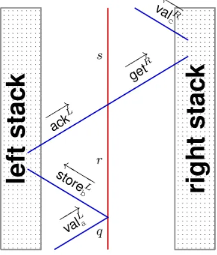
q r s −−→ val L a ←−−−− store L b −−→ ack L −−→ get R ←−− valR c FIGURE 3Implementing the sequence of transitions of Tab. 1.
Figure 3 shows how the state is encoded in-between two stacks (these are distinct; there is no common meta-signal). To distinguish the meta-signals from each stack, exponent L and R are used. The stacks record the words before and after the head. The symbol under the head is the one about to
collide with the symbol encoding the state. The side from which it comes depends only on the direction associated to the state by δM.
Transition Inverse transition δM(...) = (q, ←) δM−1(q) = (..., →) δW(q, a) = (r, b) δW−1(r, b) = (q, a) δM(r) = (s, →) δ−1M(s) = (r, ←) δW(s, c) = ... δW(...) = (s, c) TABLE 1 Sequence of transitions.
The example in Fig. 3 corresponds to the sequence of transitions on Tab. 1. The machine is on state q after a left move, so that the read symbol comes from the left stack. State r means a right move so that the letter written on the transition on q has to be sent to the left. On receiving the acknowledge from the left, r turns to s and sends the get signal to the right stack.
The reversible stack is conceived in a vertically symmetric way: the ac-knowledge and the get are symmetric. This is the same symmetry as in the expressions of the transitions on M and M−1.
Formally, there is a stack value (and associated meta-signals) for each sym-bol and a null-speed meta-signal for each state. The collision rules generated for writing transitions are given on Tab. 2.
δM( r) = ( ., ← ) δM( r) = ( ., → ) δ−1 M( q ) = ( ., ← ) { q, ←−− valL a} → { r, −−−−→ storeR b } { q, ←−− valL a } → { r, ←−−−− storeL b} δ−1M( q ) = ( ., → ) { q, −−→ valR a } → { r, −−−−→ storeR b } { q, −−→ valR a } → { r, ←−−−− storeL b}
(a) write transition δW(q, a) = (r, b)
δM( r ) = ( s, → ) { r,−−→ackL } → { s,−−→getR } δM( r ) = ( s, ← ) { r,←−−−ackR } → { s,←−−getL } (b) move transitions TABLE 2
From the properties of δW and δM, it is clear that the generated collision
rules are one-to-one. The signal machine is reversible. Moreover, the con-struction only involves collisions of two signals that generate two signals. The machine is conservative.
Special care has to be taken for states that are not moving for M−1: the
halting and initial states. For the initial state, just set the moving direction as desired. For halting states, some collisions are left undefined. They can be defined with new meta-signals that are left unmodified by the shrinking structure and exit on the left.
5 STRUCTURE
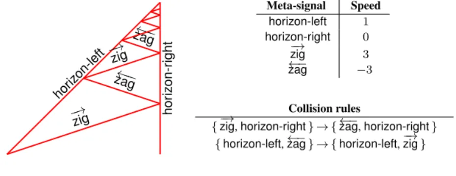
The shrinking structure depicted in Fig. 4 is briefly presented. It is fractal and accumulates to a single point.
Two signals, horizon-left and horizon-right, are getting closer and closer and would make a collision. In-between them, there is an infinite sequence of zigzagging signals,−→zig and←−−zag. This never-ending sequence is time-bounded and provide the fractal Zeno scale.
hor izon-left −→ zig ←−− zag −→ zig ←−− zag hor iz on-r ight Meta-signal Speed horizon-left 1 horizon-right 0 −→ zig 3 ←− zag −3 Collision rules
{−zig, horizon-right→ } → {←−zag, horizon-right} { horizon-left,←−zag} → { horizon-left,−zig→}
FIGURE 4 Shrinking structure.
As depicted, 4 meta-signals and 2 collision rules are enough to generate an accumulation. Accumulation is an important and common phenomenon in AGC.
6 EMBEDDING
Embedding into the structure is done as follows. The gray zone on Fig. 5 is any computation that is spatially bounded. On the right, it is displayed embedded inside the structure. The whole infinite gray computation should be inserted inside a bounded duration. This is done through an unending down-scaling presented below.
(a) bounded computation (b) partitioned (c) embedded
FIGURE 5
Shrinking a spatially bounded computation.
The gray zone is partitioned into triangular zones. The embedding alter-nates between these zones. In the triangular zone pointing right, the gray zone is bend. In the triangular zone pointing left, the grey zone is unbend.
Moreover, by construction, each triangle with the same orientation is half the size of the previous one with the same orientation. By ensuring that each time, the space-time diagram is also scaled down by half, then all the trian-gles, rescaled to scale 1 have the same size and composed the gray computa-tion as on Fig. 5(b).
Various geometric modifications can be produced by modifying the speed or the initial configuration: for example, if the initial configuration is scaled by one half, so is the space-time diagram. Another example is to take a sig-nal machine and multiply by two all speeds. The same initial configuration generates a space-time diagram which is scaled by one half on the temporal axis.
Transformations made on speed reflect on the diagram since it is actually drawnby the signals. A more complex construction is to consider two non parallel axis and use one as a frontier and the other for scaling as depicted on Fig. 6.
Figure 6(a) shows how the new speed are computed (as explained below). Figure 6(b) displays a grid to show how space-time is shrunk: the axis for this grid are parallel to the frontier vectors and at each crossing the other axis is scaled down by one half.
1 1 1 2 1 1 1 2 1 2 (a) Computations −→ zig ←−− zag (b) With grid FIGURE 6
Scaling by one half in two steps.
On Fig. 6(a), the thick lines are used as frontiers between the various zones. The directions of two frontiers are the ones used for scaling. The incoming signal at the bottom get decomposed, considered as a vector, as a sum of two vectors according to the two axis. If there were no modification, it would have followed the dotted path. But since it scaled by one half on one direction, it follows the dashed path. Passing through the second frontier, the modification is done on the other direction. So that, altogether, it is scaled by one half in both directions, thus it regains its original speed but the space-time diagram is scaled by one half!
The fact that the coordinate on the direction of the axis is not modified is very important since it ensures that the space-time diagram connects exactly on the frontier.
The speeds for dashed meta-signals are computed as follows. For each original meta-signal, µ, one meta-signal—dashed version— is added, µ′, its
speed is computed from the original one, ν, by the following formula: 3αν − α2
3α − ν
where α is the speed of−→zig (and the opposite of←−−zag). This is a bijection over the rational numbers in (−α, α).
To bent and unbent µ, the following collision rules are added: {−→zig, µ} → { µ′,−→zig} and { µ′, ←−−zag} → {←−−zag, µ}
Collision might happen in the bent zone, so that for each collision rule { σ1, . . . , σn} → { µ1, . . . , µp}, a bent version must be provided:
{ σ1′, . . . , σ′n} → { µ′1, . . . , µ′p}
moreover, a collision may happen exactly on the frontier, so that the following collision rules must also be added:
{−→zig, σ1, . . . , σn} → { µ′1, . . . , µ′p, −→ zig} and { σ′ 1, . . . , σ′n, ←−− zag} → {←−−zag, µ1, . . . , µp}
Signals−→zig and←−−zag are used for the frontier. There should not be any faster signal. The structure directly ensures that they are regenerated so as to provide the infinite acceleration.
The zone above and the zone below should not meet. In our construction, this is ensured because the TM simulation is bounded (they never go beyond horizon-left and horizon-right).
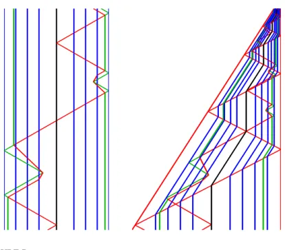
Finally, a computation and its shrinking version are displayed on Fig. 7.
REFERENCES
[1] Andrew Adamatzky, editor. (2002). Collision based computing. Springer Lon-don.
[2] Hajnal Andréka, István Németi, and Péter Németi. (2009). General relativistic hypercomputing and foundation of mathematics. Nat. Comput., 8(3):499–516. [3] Charles H. Bennett. (1973). Logical reversibility of computation. IBM J. Res.
Dev., 6:525–532.
[4] Charles H. Bennett. (1988). Notes on the history of reversible computation. IBM J. Res. Dev., 32(1):16–23.
FIGURE 7 All together.
[5] Charles H. Bennett. (August 1989). Time/space trade-offs for reversible com-putation. SIAM Journal on Computing, 18(4):766–776.
[6] Jack B. Copeland. (2002). Accelerating Turing machines. Minds & Machines, 12(2):281–300.
[7] Jean-Christophe Dubacq. (1995). How to simulate Turing machines by invert-ible 1d cellular automata. International Journal of Foundations of Computer Science, 6(4):395–402.
[8] Jérôme Durand-Lose. (1997). Intrinsic universality of a 1-dimensional reversible cellular automaton. In STACS ’97, number 1200 in LNCS, pages 439–450. Springer.
[9] Jérôme Durand-Lose. (2001). Representing reversible cellular automata with reversible block cellular automata. In Robert Cori, Jacques Mazoyer, Michel Morvan, and Rémy Mosseri, editors, Discrete Models: Combinatorics, Compu-tation, and Geometry, DM-CCG ’01, volume AA of Discrete Mathematics and Theoretical Computer Science Proceedings, pages 145–154.
[10] Jérôme Durand-Lose. (2005). Abstract geometrical computation for black hole computation (extended abstract). In M. Margenstern, editor, Machines, Compu-tations, and Universality (MCU ’04), number 3354 in LNCS, pages 176–187. Springer.
[11] Jérôme Durand-Lose. (2006). Abstract geometrical computation 1: Embedding black hole computations with rational numbers. Fund. Inf., 74(4):491–510. [12] Jérôme Durand-Lose. (2006). Reversible conservative rational abstract
geomet-rical computation is Turing-universal. In Arnold Beckmann and John V. Tucker, editors, Logical Approaches to Computational Barriers, 2nd Conf. Computabil-ity in Europe (CiE ’06), number 3988 in LNCS, pages 163–172. Springer. [13] Jérôme Durand-Lose. (2008). Black hole computation: implementation with
signal machines. In C. S. Calude and J. F. Costa, editors, International Work-shop Physics and Computation, Wien, Austria, Agust 25-28, Research Report CDMTCS-327, pages 136–158.
[14] Jérôme Durand-Lose. (2008). The signal point of view: from cellular automata to signal machines. In Bruno Durand, editor, Journées Automates cellulaires (JAC ’08), pages 238–249.
[15] Jérôme Durand-Lose. (2009). Abstract geometrical computation 3: Black holes for classical and analog computing. Nat. Comput., 8(3):455–472.
[16] John Earman and John D. Norton. (1993). Forever is a day: supertasks in Pitowsky and Malament-Hogarth spacetimes. Philos. Sci., 60(1):22–42. [17] Gábor Etesi and Istvan Németi. (2002). Non-Turing computations via
Malament-Hogarth space-times. Int. J. Theor. Phys., 41(2):341–370. gr-qc/0104023.
[18] Edward F. Fredkin and Tommaso Toffoli. (1982). Conservative logic. Int. J. Theor. Phys., 21, 3/4:219–253.
[19] Masami Hagiya. (2005). Discrete state transition systems on continuous space-time: A theoretical model for amorphous computing. In Cristian Calude, Michael J. Dinneen, Gheorghe Paun, Mario J. Pérez-Jiménez, and Grzegorz Rozenberg, editors, Unconventional Computation, 4th International Conference, UC ’05, Sevilla, Spain, October 3-7, 2005, Proceedings, volume 3699 of LNCS, pages 117–129. Springer.
[20] Joel David Hamkins and Andy Lewis. (2000). Infinite time Turing machines. J. Symb. Log., 65(2):567–604. arXiv:math.LO/9808093.
[21] Mark L. Hogarth. (1994). Non-Turing computers and non-Turing computability. In Biennial Meeting of the Philosophy of Science Association, pages 126–138.
[22] Mark L. Hogarth. (2004). Deciding arithmetic using SAD computers. Brit. J. Philos. Sci., 55:681–691.
[23] Giuseppe Jacopini and Giovanna Sontacchi. (1990). Reversible parallel compu-tation: an evolving space-model. Theoret. Comp. Sci., 73(1):1–46.
[24] Yves Lecerf. (1963). Machines de Turing réversibles. Récursive insolubilité en n ∈ N de l’équation u = θn
u, où θ est un isomorphisme de codes. Comptes rendus des séances de l’académie des sciences, 257:2597–2600.
[25] Seth Lloyd and Jack Ng, Y. (November 2004). Black hole computers. Scientific American, 291(5):31–39.
[26] Ralph C. Merkle. (1993). Reversible electronic logic using switches. Nanotech-nology, 4(1):20–41.
[27] Kenichi Morita. (June 1990). A simple construction method of a reversible finite automaton out of Fredkin gates, and its related problem. Transactions of the IEICE, E 73(6):978–984.
[28] Kenichi Morita. (1996). Universality of a reversible two-counter machine. The-oret. Comp. Sci., 168(2):303–320.
[29] Kenichi MORITA, Akihiko Shirasaki, and Yoshifumi Gono. (March 1989). A 1-tape 2-symbol reversible Turing machine. Transactions of the IEICE, E 72(3):223–228.
[30] István Németi and Hajnal Andréka. (2006). Can general relativistic computers break the Turing barrier? In Arnold Beckmann, Ulrich Berger, Benedikt Löwe, and John V. Tucker, editors, Logical Approaches to Computational Barriers, 2nd Conf. on Computability in Europe, CiE ’06, volume 3988 of LNCS, pages 398– 412. Springer.
[31] István Németi and Gyula Dávid. (2006). Relativistic computers and the Turing barrier. Appl. Math. Comput., 178(1):118–142.
[32] Izumi Takeuti. (2005). Transition systems over continuous time-space. Electr. Notes Theor. Comput. Sci., 120:173–186.
[33] Tommaso Toffoli. (1977). Computation and construction universality of re-versible cellular automata. J. Comput. System Sci., 15:213–231.
[34] Tommaso Toffoli. (1980). Reversible computing. In ICALP, volume 85 of LNCS, pages 632–644. Springer.
[35] Tommaso Toffoli and Norman Margolus. (1990). Invertible cellular automata: a review. Phys. D, 45:229–253.