HAL Id: hal-00940743
https://hal.inria.fr/hal-00940743v3
Submitted on 11 Apr 2016
HAL is a multi-disciplinary open access
archive for the deposit and dissemination of sci-entific research documents, whether they are pub-lished or not. The documents may come from
L’archive ouverte pluridisciplinaire HAL, est destinée au dépôt et à la diffusion de documents scientifiques de niveau recherche, publiés ou non, émanant des établissements d’enseignement et de
Efficiently navigating a random Delaunay triangulation
Nicolas Broutin, Olivier Devillers, Ross Hemsley
To cite this version:
Nicolas Broutin, Olivier Devillers, Ross Hemsley. Efficiently navigating a random Delaunay trian-gulation. Random Structures and Algorithms, Wiley, 2016, 49 (1), pp.95–136. �10.1002/rsa.20630�. �hal-00940743v3�
Efficiently Navigating a Random
Delaunay Triangulation
⇤Nicolas Broutin† Olivier Devillers‡ Ross Hemsley§
April 11, 2016
Abstract
Planar graph navigation is an important problem with significant implications to both point location in geometric data structures and routing in networks. However, whilst a num-ber of algorithms and existence proofs have been proposed, very little analysis is available for the properties of the paths generated and the computational resources required to gen-erate them under a random distribution hypothesis for the input. In this paper we analyse a new deterministic planar navigation algorithm with constant spanning ratio (w.r.t the Eu-clidean distance) which follows vertex adjacencies in the Delaunay triangulation. We call this strategy cone walk. We prove that given n uniform points in a smooth convex domain of unit area, and for any start point z and query point q; cone walk applied to z and q will access at most O(|zq|pn+log7n)sites with complexity O(|zq|pn log log n+log7n)with probability tending to 1 as n goes to infinity. We additionally show that in this model, cone walk is (log3+⇠n)-memoryless with high probability for any pair of start and query point
in the domain, for any positive ⇠. We take special care throughout to ensure our bounds are valid even when the query points are arbitrarily close to the border.
1 Introduction
Given a planar embedding of a graph G = (V, E), a source node z 2 V and a destination point q 2 R2, we consider the planar graph navigation problem of finding a route in G from z to
the nearest neighbour of q in V . In particular, we assume that any vertex v 2 V may access its coordinates in R2 with a constant time query. The importance of this problem is two-fold.
On the one hand, finding a short path between two nodes in a network is currently a very active area of research in the context of routing in networks [11, 2222, 2727]. On the other, the problem of locating a face containing a point in a convex subdivision (point location) is an important sub-routine in many algorithms manipulating geometric data structures [1111, 1212, 1818, 2323]. A number of algorithms have been proposed within each of these fields, many of which are in fact equivalent. It seems the majority of the literature in these areas is concerned with the existence
⇤The work in this paper has been partially supported by ANR blanc PRESAGE (ANR-11-BS02-003) †Projet RAP, INRIA Paris - Rocquencourt
‡Projet Geometrica, INRIA Sophia Antipolis - Méditerranée §Projet Geometrica, INRIA Sophia Antipolis - Méditerranée
of algorithms which always succeed under different types of constraints, such as the spanning ratio or the competitiveness of the algorithm, or the class of network. Apart from worst-case bounds, very little is known concerning the properties of the path lengths and running times for these algorithms under random distribution hypotheses for the input vertices. In this paper we aim to bridge the gap between these two fields by giving and analysing an algorithm that is provably efficient within both of these contexts when the underlying graph is the Delaunay triangulation.
1.1 Definitions
In the following, we define the spanning ratio of an algorithm to be the worst case ratio between the length of the path generated by the algorithm and the Euclidean distance between the source and the destination and the competitiveness the worst case ratio between the lengths of the paths produced by the studied algorithm and an optimal offline algorithm. Thus the spanning ratio is always larger than the competitiveness and a good spanning ratio imply a good competitiveness. They both may depend on the class of graphs one allows, but not the pair of source and desti-nation. Let Nd(v) denote the set of neighbours of v within d hops of v. We shall sometimes
refer to the d’th neighbourhood of a set X, to denote the set of all sites that can be accessed from a site in X with fewer than d hops. We call an algorithm c-memoryless if at each step in the navigation, it only has access to the destination q, the current vertex v and Nc(v). Some
authors use the term online to refer to an algorithm that only has access to q, the current vertex v, N1(v)and O(1) words of memory which may be used to store information about the history
of the navigation. Finally, an algorithm may be either deterministic or randomised. We define a randomised algorithm to be an algorithm that has access to a random oracle at each step.
1.2 Previous results
Graph Navigation for Point location. The problem of point location is most often studied in the context of triangulations and the algorithms are referred to as walking algorithms [1212]. A walking algorithm may work by following edges or by following incidences between neighbour-ing faces, which is equivalent to a navigation in the dual graph. There are three main algorithms that have received attention in the literature: straight walk, which is a walk that visits all tri-angles crossed by the line segment zq; greedy vertex walk, which always chooses the vertex in N1(v)which is closest to q and visibility walk which walks to an adjacent triangle if and only if
it shares the same half-space as q relative to the shared edge. It is known that these algorithms always terminate if the underlying triangulation is Delaunay [1212].
The aim is generally to analyse the expected number of steps that the algorithm requires to reach the destination under a given distribution hypothesis. Such an analysis has only been provided by Devroye et al. [1414] who succeeded in showing that straight walk reaches the desti-nation after O(kzqkpn )steps in expectation, for n random points in the unit square (here and from now on we shall use k · k to denote the Euclidean distance).11 The analysis in this case is
1Zhu also provides a tentative O pn log n bound for visibility walk [2828]. This is a proof by induction for “a random edge at distance d”. It considers the next edge in the walk and applies an induction hypothesis to try and bound the progress. Unfortunately, the new edge cannot be considered as random: each edge that is visited has been
facilitated since it is possible to compute the probability that a triangle is part of the walk without looking at the other vertices. Straight walk is online, but not memoryless since at every step the algorithm must know the location of the source point, z. It is also rarely used in practice since it is usually outperformed empirically by one of the remaining two algorithms, visibility walk or greedy vertex walk, which are both 1-memoryless [1212]. The complex dependence between the steps of the algorithm in these cases makes the analysis difficult, and it remains an important open question to provide an analysis for either of these two algorithms.
Graph Navigation for Routing. In the context of packet routing in a network, each vertex represents a node which knows its approximate location and can communicate with a selected set of neighbouring nodes. One example is in wireless networks where a node communicates with all devices within its communication range. In such cases, it is often convenient for the nodes to agree on a communication protocol such that the graph of directly communicating nodes is planar, since this can make routing more efficient. Triangulations have been used in this context due to their ability to act as spanners (the length of shortest paths in the graph, seen as curves in R2, do not exceed the Euclidean distance by more than a constant factor), and methods
exist to locally construct the full Delaunay triangulation, given some conditions on the point distribution [1717, 1919, 2424].
Commonly referenced algorithms in this field are: greedy routing, which is the same algo-rithm as greedy vertex walk, given in the context of point location; compass routing which is similar to greedy, except that instead of choosing the point in N1(v)minimising the distance to
q, it chooses the point in x 2 N1(v)minimising the angle\q, v, x, and also face routing which
is a generalisation of straight walk that can be applied to any planar graph. In this context, over-all computation time is usuover-ally considered less important than trying to construct algorithms that find short paths in a given network topology under certain memory constraints. We give a brief overview of results relating to this work.
Bose et al. [88] demonstrated that it is not possible to construct a deterministic memoryless algorithm that finds a path with constant competitiveness in an arbitrary triangulation. They also demonstrated by counter example that neither greedy routing, nor compass routing is O(1)-competitive on the Delaunay triangulation [66]. Bose and Morin [77] went on to show that there does, however, exist an online c-competitive algorithm that works on any graph satisfying a property they refer to as the ‘diamond property’, which is satisfied by Delaunay triangulations. They show this by providing an algorithm which is essentially a modified version of the straight walk. Bose and Morin also show that there is no algorithm that is competitive for the Delau-nay triangulation under the link length (the link length is the number of edges visited by the algorithm) [88].
In terms of time analysis, it appears the only relevant results are those by Devroye et al. [1414], where their results correspond with that of the straight walk, and those by Chen et al. [1010], who show that no routing algorithm is asymptotically better than a random walk when the underlying graph is an arbitrary convex subdivision.
chosen by the algorithm and the edges do not all have the same probability to be chosen at each step in the walk. Restarting the walk from a given edge is not possible either (as done in [1313]), since the knowledge that an edge is a Delaunay edge influences the local point distribution.
Navigation in the Plane. We briefly remark that for the related problem of navigation in the plane, several probabilistic results exist; for example [33] and [44]. In this context, the input is a set of vertices in the plane along with an oracle that can compute the next step given the current step and the destination in O(1) time. Although the steps are also dependent in these cases, the case of Delaunay triangulations we treat here is more delicate because of the geometry of the region of dependence implied by the Delaunay property.
1.3 Contributions
In this paper we give a new deterministic planar graph navigation algorithm which we call cone walk that succeeds on any Delaunay triangulation and produces a path which is 3.7-spanning ratio. We briefly underline the fact that our algorithm has been designed for theoretical demon-stration, and we do not claim that it would be faster in a practical sense than, for example, greedy routing or face routing. On the other hand, direct comparisons would perhaps be unfair, since greedy routing is not O(1)-competitive on the Delaunay triangulation [66] whereas we prove that cone walk is; and face routing is not memoryless in any sense, whilst cone walk is localised in the sense given by Theorem 11. In the theorems that follow, we characterise the asymptotic properties of the cone walk algorithm applied to a random input.
Let D be a smooth convex domain of the plane with area 1, and write Dn = pnD for its
scaling to area n. For x, y 2 D, let kxyk denote the Euclidean distance between x and y. Under the hypothesis that the input is the Delaunay triangulation of n points uniformly distributed in a convex domain of unit area, we prove that, for any " > 0, our algorithm is O(log1+"
n)-memoryless with probability tending to one. In the case of cone walk, this is equivalent to bounding the number of neighbourhoods that might be accessed during a step, which we deal with in the following theorem.
Theorem 1. Let Xn:={X1, X2, . . . , Xn} be a collection of n independent uniformly random
points in Dn. For z 2 Xnand q 2 Dn, let M(z, q) be the maximum number of neighbourhoods
needed to compute every step of the walk. Then, for every ✏ > 0, P⇣9z 2 Xn, q2 Dn: M (z, q) > log3+✏n
⌘ 1
n. In particular, as n ! 1, E[supz2Xn,q2DnM (z, q)] = O(log
3+✏n), for every ✏ > 0.
Also with probability close to one, we show that the path length, the number of edges and the number of vertices accessed are O( kzqk + log6n )for any pair of points in the domain. We
formalise these properties in the following theorem.
Theorem 2. Let Xn:={X1, X2, . . . , Xn} be a collection of n independent uniformly random
points in Dn. Let (z, q) denote either the Euclidean length of the path generated by the cone
walk from z 2 Xnto q 2 Dn, its number of edges, or the number of vertices accessed by the
algorithm when generating it. Then there exist constants C ,Ddepending only on and on the
shape of D such that, for all n large enough, P ✓ 9z 2 Xn, q2 Dn : (z, q) > C ,D· kzqk + 4(1 + p kzqk) log6n ◆ 1 n.
In particular, as n ! 1, E sup z2Xn, q2Dn (z, q) = O(pn ).
Finally, we bound the computational complexity of the algorithm, T (z, q).
Theorem 3. Let Xn:={X1, X2, . . . , Xn} be a collection of n independent uniformly random
points in Dn. Then in the RAM model of computation, there exists a constant C depending only
on the shape of D and the particular implementation of the algorithm such that for all n large enough, P ✓ 9z 2 Xn, q 2 Dn : T (z, q) > C· kzqk log log n + (1 + p kzqk) log6n ◆ 1 n. In particular, as n ! 1, E sup z2Xn, q2Dn T (z, q) = O(pn log log n ).
Remark 1. The choice of the initial vertex is never discussed. However, previous results show that choosing this point carefully can result in an expected asymptotic speed up for any graph navigation algorithm [2323].
1.4 Layout of the paper
In Section 22, we give a precise definition of the cone walk algorithm and prove some important geometric properties. In Section 33, we begin the analysis for the cone walk algorithm applied to a homogeneous planar Poisson process. To avoid problems when the walk goes close to the boundary, we provide an initial analysis which assumes that the points are sampled from a disc with the query point at its centre. This analysis is then extended to arbitrary query points in the disc and also to other convex domains in Section 44. In Section 55, we prove estimates about an auxiliary line arrangement which are crucial to proving the worst-case probabilistic bounds in Theorems 11and 33. Finally, we compare our findings with computer simulations in Section 66.
2 Algorithm and geometric properties
We consider the finite set of sites in general position (so that no three points of the domain are co-linear, and no four points are co-circular), X ⇢ R2 contained within a compact convex
domain D ⇢ R2. Let DT(X) be the Delaunay triangulation of X, which is the graph in which
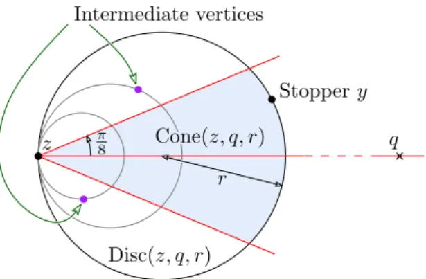
three sites x, y, z 2 X form a triangle if and only if the disc with x, y and z on its boundary does not contain any site in X. Given two points z, q 2 R2 and a number r 2 R we define
Disc(z, q, r)to be the closed disc whose diameter spans z and the point at a distance 2r from zon the ray zq. Finally, we define Cone(z, q, r) to be the sub-region of Disc(z, q, r) contained within a closed cone of apex z, axis zq and half angle⇡
Stopper y Disc(z, q, r) z q Intermediate vertices Cone(z, q, r) r ⇡ 8
Figure 1: Choosing the next vertex.
2.1 The cone walk algorithm
Given a site z 2 X and a destination point q 2 D, we define one step of the cone walk algorithm by growing the region Cone(z, q, r) anchored at z from r = 0 until the first point y 2 X is found such that the region is non-empty. Once y has been determined, we refer to it as the stopper. We call the region Cone(z, q, r) for the given r a search cone, and we call the associated disc Disc(z, q, r)the search disc (see Figure 11). The point y is then selected as the anchor of a new search cone Cone(y, q, ·) and the next step of the walk begins. See Figure 22for an example run of the algorithm.
To find the stopper using only neighbour incidences in the Delaunay triangulation, we need only access vertices in a well-defined local neighbourhood of the search disc. Define the points X\ Disc(z, q, r) \ {z, y} to be the intermediate vertices. The algorithm finds the stopper at each step by gradually growing a disc anchored at z in the direction of the destination, adding the neighbours of all vertices in X intersected along the way. This is achieved in practice by maintaining a series of candidate vertices initialised to the neighbours of z and selecting amongst them the vertex defining the smallest search disc at each iteration. Each time we find a new vertex intersecting this disc, we check to see if it is contained within Cone(z, q, 1). If it is, this point is the next stopper and this step is finished. Otherwise the point must be an intermediate vertex and we add its neighbours to the list of candidate vertices. This procedure works because the intermediate vertex defining the next largest disc is always a neighbour of one of the intermediate vertices that we have already visited during the current step (see Lemma 55).
We terminate the algorithm when the destination q is contained within the current search disc for a given step. At this point we know that one of the points contained within Disc(z, q, r) is a Delaunay neighbour of q in DT(X [ {q}). We can further compute the triangle of DT(X) containing the query point q (point location) or find the nearest neighbour of q in DT(X) by simulating the insertion of the point q into DT(X) and performing an exhaustive search on the neighbours of q in DT(X [ {q}).
We will sometimes distinguish between the visited vertices, which we take to be the set of all sites contained within the search discs for every step and the accessed vertices, which we define to be the set of all vertices accessed by the cone-walk algorithm. Thus the accessed vertices are
the visited vertices along with their 1-hop neighbourhood.
The pseudo-code below gives a detailed algorithmic description of the CONE-WALK
al-gorithm. We take as input some z 2 X, q 2 D and return a Delaunay neighbour of q in DT(X[ {q}). Recalling that N1(v)refers to the Delaunay neighbours of v 2 DT(X) and
ad-ditionally defining NEXT-VERTEX(S, z, q)to be the procedure that returns the vertex in S with the smallest r such that Disc(z, q, r) touches a vertex in S and IN-CONE(z, q, y)to be true when y 2 Cone(z, q, 1).
CONE-WALK(z, q) 1 Substeps = {z} 2 Candidates = N1(z) 3 while true
4 y = NEXT-VERTEX(Candidates[ {q}, z, q) 5 if IN-CONE(z, q, y)
6 if y = q
7 //Destination reached.
8 return NEXT-VERTEX(Substeps, q, z) 9 // yis a stopper 10 z = y 11 Substeps = {z} 12 Candidates = N1(z) 13 else 14 // yis an intermediate vertex. 15 Substeps = Substeps[ {y}
16 Candidates = Candidates[ N1(y)\ Substeps
2.2 Path Generation
We note that the order in which the vertices are discovered during the walk does not necessarily define a path in DT(X). If we only wish to find a point of the triangulation that is close to the destination (for example, in point location), this is not a problem. However, in the case of routing, a path in the triangulation is required to provide a route for data packets. To this end, we provide two options that we shall refer to as SIMPLE-PATHand COMPETITIVE-PATH.
SIMPLE-PATH is a simple heuristic that can quickly generate a path that is provably short on
average. SIMPLE-PATHmay have an unbounded spanning ratio in some pathological situations
where the path makes zig-zag, it has only a good expected spanning-ratio. COMPETITIVE-PATH
is slightly more complex from an implementation point of view, however we show that for any possible input the algorithm will always generate a path of constant spanning ratio whilst still maintaining the same asymptotic behaviour under the point distribution hypotheses explored in Section 33.
SIMPLE-PATH A simple way to generate a valid path is to keep a predecessor table for each
vertex. We start with an empty table at the beginning of each step, and then every time we access a new vertex, we store it in the table along with the vertex that we accessed it from. To trace a path back, we simply follow the predecessors.
COMPETITIVE-PATH Let Zi for i > 0, be the ith stopper in the walk thus, Zi is the stopper
found at step i) and Z0 := z. For a path to have a good spanning ratio, it should at least
have a good spanning ratio locally: for each step, there should be a bound on the length of the path generated between Zi and Zi+1, which does not depend on the points in the search
disc. To construct a path verifying this property, we use the fact that the stretch factor of the Delaunay triangulation is bounded above by a constant, . This means that for any two sites x, y, there exists a path from x to y in the Delaunay triangulation for which the sum of the lengths of the edges is at most kxyk. Currently the literature gives us that the stretch factor is in [1.5932, 1.998] [2525, 2626]. Clearly this implies that there exists a path between Ziand Zi+1
with total length at most kZiZi+1k. Moreover, for = 1.998, Xia proved that there exists such
a path using only vertices of the Delaunay edges crossing the line segment xy, and such edges have at least one vertex in the intermediate vertices bewteen Zi and Zi + 1. We use Dijkstra’s
algorithm to find the shortest path between Zi and Zi+1which uses only intermediate vertices
between Zi and Zi+1and their neighbors. The resulting path implicitly has stretch bounded by
. We show in Lemma 44that this algorithm results in a bound for the spanning ratio for the full path.
Lemma 4. CONE-WALKhas 3.7-spanning ratio when the COMPETITIVE-PATH algorithm is
used to generate the path in DT(X)
Proof. Let Zi, Zi+1 be the stoppers of two consecutive steps defined by the algorithm. The
stretch factor bound guarantees that the path generated between Ziand Zi+1has length bounded
by kZiZi+1k, meaning that the longest path can have stretch at most P⌧ 1i=0 kZiZi+1k/kzqk
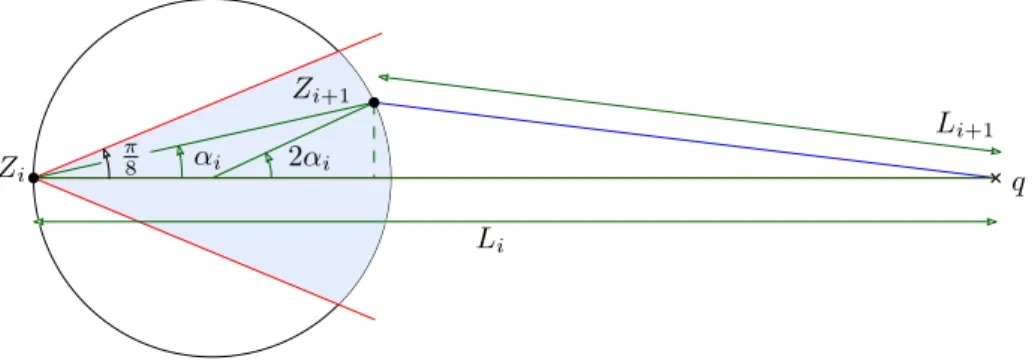
where ⌧ is the number of steps in the walk. We bound this sum by observing that kZiZi+1k
2 cos⇡8 · (kZiqk kZi+1qk), which follows from Figure 88. Finally, no path defined by the
algorithm can be longer than
⌧ 1 X i=0 kZiZi+1k 2 cos⇡8 ⌧ 1 X i=0 kZiqk kZi+1qk 2 cos⇡8 · kzqk
Thus the path has a spanning ratio of c for c := 2 cos⇡
8 4 cos⇡8 3.7.
2.3 Complexity
In this section we give deterministic bounds on the number of operations required to compute CONE-WALK(z, q)within the RAM model of computation. In this model, accessing, comparing and performing arithmetic on points is treated as atomic. We will use these deterministic bounds to extract probabilistic bounds under certain distribution assumptions in Section 3.43.4. For now, we focus on a single step of the walk starting from y 2 X, and resulting in a disc with radius r. Let k be the number of points intersecting the disc Disc(y, q, r) and m be the number of edges in DT(X) intersecting @ Disc(y, q, r) (where we use the notation @A to denote the boundary of A) .
We note that every intermediate vertex will add its neighbours to the list of Candidates when visited. Each of these insertions can be associated with a single edge of DT(X) intersect-ing Disc(y, q, r) (with multiplicity two for each ‘internal’ edge, since they are accessed from
q
Z0 Z1 Z2 Z3 Z4 Z 1 R1 S1Figure 2: An example of cone walk. The points (Zi)i>0are the stoppers (or sometimes, the
steps) and the points within each circle are the intermediate vertices. The shaded conic regions are the cones, and the set of outer circles for each of the steps in the diagram is referred to as the discs.
both sides). By the Euler relation, the total number of such insertions for one step is thus at most 3(m + 2k). In addition, we observe that when moving from one intermediate vertex to the next, a search in the list of Candidates is required. A simple linear search requires O(m + k) operations for each intermediate vertex. Combining this with the above, we achieve a bound of O(k(m + k))operations for one step. This bound may be improved by replacing Candidates with a priority queue keyed on the associated search-disc radius of each candidate, which yields a simple improvement to O(k log(m + k)).
For the path generation algorithms, we observe that SIMPLE-PATHonly requires a constant
amount of processing per vertex accessed to generate the predecessor table and O(k) time to output the path at the end of each step, so the asymptotic running time is not affected by its inclusion. COMPETITIVE-PATHis slightly more complicated since it uses Dijkstra’s algorithm
on the k points in the search disc and their neighbors. Let k0 be the number of neighbors, the
complexity is O((k + k0) log(k + k0)).
2.4 Geometric properties
We now prove a series of geometric lemmata giving properties of steps in the walk. We begin with a small lemma that will guarantee that we never get ‘stuck’ when performing a search for the next step, thus demonstrating correctness of the algorithm. The following two ‘overlapping’ lemmata allow us to establish which regions may be considered independent in a probabilistic sense and will be important in Section 33. Finally we provide a ‘stability’ result, which will help us to bound the region in which a destination point may be moved without changing the
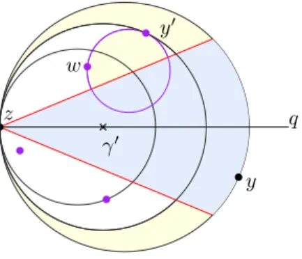
z y q 0 y0 w
Figure 3: We observe that y0 has always a Delaunay neighbour in Disc(z, q, r), where r is the
radius ensuring y 2 @Disc(z, q, r).
sequence of steps taken by the algorithm. This will be important when we enumerate the number of different walks possible for a given set of input points.
2.4.1 Finding a Delaunay path within the discs
Lemma 5 (Path finding lemma). Let q 2 D, z 2 X and y0 2 X with associated disc Disc(z, q, r0).
Suppose there exists an r > 0 such that (Disc(z, q, r0)\ Disc(z, q, r)) \ X = {y0}. Then there
exists a point in Disc(z, q, r) that is a Delaunay neighbour of y0.
Proof. Let 0 be the centre of Disc(z, q, r0). We grow Disc(y0, 0, ⇢) ⇢ Disc(z, q, r0) until
we hit a point w in X. The point w is always contained within Disc(z, q, r) because z is on the border of Disc(z, q, r). Since the interior of the Disc(y0, 0, ⇢)is empty, w is a Delaunay
neighbour of y0. See Figure 33.
Corollary 6. Let q 2 D, z 2 X with y 2 X its associated stopper satisfying y 2 @Cone(z, q, r). Then there is a path of edges of DT(X) from z to y contained within Disc(z, q, r).
2.4.2 Independence of the search cones
When growing a new search cone, it is important to observe that it does not overlap any of the previous search cones, except at the very end of the walk. This is formalised by the following lemma.
Lemma 7 (Non-overlapping lemma). Let z and y be two points of X and r > 0 such that Cone(z, q, r)has y on its boundary. If kzqk > (2 +p2 )r then Disc(z, q, r) does not intersect the search cone Cone(y, q, 1) issued from y nor any other search cone for any subsequent step of the walk.
Proof. Assume without loss of generality that y lies to the left of line zq and consider the con-struction given in Figure 44. Let denote the angle between the tangent to Disc(z, q, r) at y and the ray bordering Cone(y, q, 1). Cone(y, q, 1) and Disc(z, q, r) do not intersect provided that
⇡ 8 Cone(y, q,1) ⇡ 4 ⇡ 8 r Disc(z, q, r) ⇡ 8 z ⇡8 q z0 Cone(z, q, r) y
Figure 4: For the proof of Lemma 77.
Disc(z, q, r) q y y0 ⇢ Cone(y, q, ⇢) Disc(z, q, r)\ Disc(y, q, ⇢) ⇢ Cone(z, q, r)
Disc(y, q, ⇢)
z
Cone(z, q, r)
Figure 5: For the proof of Lemma 88.
0. Placing y at the corner of Cone(z, q, r) maximizes , in which case we have > 0if and only if q is to the right of z0, the point symmetrical to z with respect to the line through y
perpendicular to zq. Elementary computations then yield the result. Since the whole sequence of search cones following the one issued from y remains in Cone(y, q, 1), Disc(z, q, r) does not intersect any of these search cones, and the result follows.
2.4.3 Independence of the search discs
When growing the search disc region, the new search disc may overlap previous search discs but only in their cone parts. This is formalised by the following lemma:
Lemma 8 (Overlapping lemma). Let z and y be two points such that Cone(z, q, r) has y on its boundary. Then if the search disc Disc(y, q, ⇢) issued from y does not contain q, it does not intersect Disc(z, q, r) \ Cone(z, q, r).
Proof. By symmetry we observe that Disc(y, q, ⇢) only intersects the point y0, the point y
z
s
Figure 6: For the proof of Lemma 99. For a given step z, moving the destination in the shaded sector will always result in the same stopper, s, being chosen for the next step.
the algorithm terminates as soon as the current search disc touches q, q is never contained within Disc(z, q, ⇢)and thus this can never happen.
2.4.4 Stability of the walk
In the following lemma we are interested in the stability of the sequence of steps to reach q. Lemma 9 (Invariance lemma). For an n-set X ✓ R2, there exists an arrangement of half-lines
⌅ = ⌅(X)such that the associated subdivision of the plane has fewer than 2n4cells, and such
that the sequence of steps used by the cone walk algorithm from any vertex of X does not change when the aim q moves in a connected component of R2\ ⌅.
Proof. Take a point z 2 X and consider Sz, the set of all possible stoppers defined by Cone(z, q, r)
for some q 2 D and r > 0. Each s 2 Szdefines a unique sector about z such that moving a point
in the given sector does not change the stopper (see Figure 66). We then create an arrangement by adding a ray on the border of every sector for each point z 2 X. The resulting arrangement has the property that moving the destination point q within one of the cells of the arrangement does not change the stopper of any step for any possible walk. Clearly, |Sz| n 1for all
z2 X, and each sector is bounded by at most two rays, thus there are at most 2n(n 1) rays in the arrangement. Since an arrangement of m lines has at most m2+m+2
2 cells the result follows
[see, e.g., 2020, p. 127].
3 Cone walk on Poisson Delaunay in a disc
Our aim in this section is to prove the main elements towards Theorem 33, which we go on to complete in Section 44. Our ultimate goal is to prove bounds on the behaviour of the cone walk for the worst possible pair of starting point and query when the input sites are generated by a
homogeneous Poisson process in a compact convex domain. Achieving this requires first strong bounds on the probability that the walk behaves badly for a fixed start point and query. One then proves the worst-case bounds by showing that to control every possible run of the algorithm, it suffices to bound the behaviour of the walk for enough pairs of starting points and query; this relies crucially on the arrangement of Lemma 99. The tail bounds required in the second stage of the proof may not be obtained from Markov or Chebyshev’s inequalities together with mean or variance estimates only, and we thus need to resort to stronger tools.
Our techniques rely on concentration inequalities [99, 1515, 1616, 2121]. Most of the bounds we obtain (for the number of steps and the number of visited sites) follow from a representation as a sum of random variables in which the increments can be made independent by a simple and natural conditioning. The bounds on the complexity of the algorithm CONE-WALKare slightly
trickier to derive because there is no way to make the increments independent.
For the sake of presentation, we introduce two simplifications which we remove in Sec-tion 44. First, we start by studying the walk in the disc Dnof area n where the query is at the
centre. These choices for Dnand q ensure that for any z 2 Dnand any r
p
n/⇡, we have Disc(z, q, r) ⇢ Dn. Note that since the distance to the aim is decreasing, the disc is precisely
the effective domain where the walk from z and aiming at q takes place.
Then, we introduce independence between the different regions of the domain by replac-ing the collection of independent points Xnby a (homogeneous) Poisson point process and
consider DT( ). Recall that a Poisson point process of intensity 1 is a random collection of points ⇢ Dnsuch that with probability one, all the points are distinct, for any two Borel sets
R, S ✓ Dn, the number of points | \ R| is distributed like a Poisson random variable whose
mean is the area A(R) of R, and if R \ S = ? then | \ R| and | \ S| are independent. On many occasions, it is convenient to consider conditioned to have a point located at z2 D and we let zbe the corresponding random point set. Classical results on Poisson point
processes ensure that z\ {z} is distributed like , so that one can take z = [ {z}, for
independent of z [see, e.g., 11, Section 1.4].
3.1 Preliminaries
We establish the following notation (see Figure 22). Let Z = (Zi, i > 0)denote the sequence
of stoppers visited during the walk with Z0 := z. Let Li = kZiqk denote the distance to the
destination q. The distance Li is strictly decreasing and the point set is almost surely finite,
thus ensuring that the walk stops after a finite number of steps , at which point we have Z = q.
For x > 0, we also let (x) be the number of steps required to reach a point within distance x of the query. Thus, using the fact that Li is decreasing, we get that i < (x) if and only if Li> x.
The important parameters needed to track the location and progress of the walk are the radius Ri
such that Zi+1 2 @Cone(Zi, q, Ri), and the angle ↵i between Ziqand ZiZi+1. Disc(Zi, q, Ri)
may contain several points of , let ⌧idenote | Disc(Zi, q, Ri)\ {Zi, Zi+1} \ | the number of
such points and Nithe number of these points along with their Delaunay neighbours.
In order to compute the walk efficiently, the algorithm presented gathers a lot of information. In particular, we access all the points in Disc(Zi, q, Ri)and their neighbours. For the analysis,
contains the necessary information for the walk to be a measurable process. Let Fi denote the
information consisting of (the -algebra generated by) the locations of the points of contained in [i
j=0Disc(Zj, q, Rj). Finally, we shall write !nto denote a sequence satisfying !n log n.
(We do not really need an upper bound on !n, but of course, if it is too large, some of the results
become vacuus; one could typically think of it as log n or a polylog.)
We often need to condition on the size of the largest empty ball within the process n. This
is dealt with in the following lemma.
Lemma 10. Let b(x, r) denote the closed ball of radius r centred at x. Then 8c > 0, ⇠ > 0, P 9x 2 Dn: b(x, c !1/2+⇠n )\ n=? exp
⇣
!1+⇠n ⌘ for n sufficiently large.
Proof. We have
P(9x 2 Dn: b(x, c !n1/2+⇠)\ n=?) P(9B 2 P : B \ n=?),
where P is any maximal packing of Dnwith balls B of radius 12c !n1/2+⇠centred in Dn. (Here,
by packing, we mean that one could not add any ball to the collection, but we do not enforce the balls to be fully contained in Dn, only that their centers lie in Dn; so in particular, such a
packing is never empty, even if the balls are larger than Dn.) If the radius of curvature of Dnis
lower bounded by c !n1/2+⇠(which happen for n large enough) such a ball B contains a ball of
radius 1 4c !
1/2+⇠
n entirely inside Dn, For n large enough, any such packing contains at most n
balls and we have
P(9x 2 Dn: b(x, c !n1/2+⇠)\ n=?) n exp ⇡412 c2!n1+2⇠ exp
⇣
!n1+⇠⌘. 3.1.1 The size of the discs
If the search cone Cone(Zi, q,1) does not intersect any of the previous discs, the region which
determines Ri+1is ‘fresh’ and Ri+1is independent of Fi. Lemma 77provides a condition which
guarantees independence of the search cones. To take advantage of it, we write ⇠ := 2 +p2, and for i 0, define the event
Gi :={8j i + 1, Rj < !n/⇠}, (1)
Then if the event G?
i := Gi\{Li !n} occurs; for every j i, the search-cone Cone(Zj, q,1)
does not intersect any of the regions Disc(Zk, q, Rk), 0 k < j, and the corresponding
vari-ables (Rj, ↵j), 0 j i + 1 are independent. Although it might seem like an odd idea, G?i
does include some condition on Ri+1; this ensures that on G?i, we have Li+1> Li 2Ri+1> 0,
so that i + 1 is not the last step. So for x > 0 we have
P(Ri+1> x| Fi, G?i) =P( \ Cone(Zi, q, x)\ {Zi} = ? | Fi, G?i)1{⇠x!n}
where A denotes the area of Cone(z, q, 1) which is the shaded region in Figure 11. Indeed, conditional on Fiand G?i, | \ Cone(Zi, q, x)\ {Zi}| is a Poisson random variable with mean
Ax2where A := 2⇣cos⇡ 8sin ⇡ 8 + ⇡ 8 ⌘ = p 2 2 + ⇡ 4. (3)
We will repeatedly use the conditioning on Gi to introduce independence, and it is important
to verify that Gi indeed occurs with high probability. For Gi to fail, there must be a first step
jfor which Rj !n/⇠. Writing Gci for the complement of Gi and defining G 1to be a void
conditioning: provided that i = O(n) (which will always be the case in the following) P(Gc
i)
X
0ji+1
P(Rj !n/⇠| Gj 1)
exp log O(n) A!2n/⇠2
exp⇣ !n3/2⌘ (4)
for all n large enough since !n log n.
Remark about the notation. It is convenient to work with an “ideal” random variable that is not constrained by the location of the query or artificially forced to be at most !n/⇠, and we define
R by P(R x) = exp Ax2 for x 0. In the course of the proof, we use multiple other
such ideal random variables, to distinguish them from the ones arising from the actual process, we use calligraphic letters to denote them.
3.1.2 The progress for one step
We now focus on the distribution of the angle\qZiZi+1 and by extension the progress made
during one step in the walk. Let Cone↵(z, q, r)be the cone of half angle ↵ with the same apex
and axis as Cone(z, q, r). For S ⇢ R2, let A(S) denote its area. On the event G?
i, Zi+16= q and
↵i+1is truly random and its distribution is symmetric and given by (see Figure 77):
P(|↵i+1| < x | Ri+1= r,Fi, G?i) = lim" !0 A(Conex(Zi, q, r + ")\ Conex(Zi, q, r)) A(Cone(Zi, q, r + ")\ Cone(Zi, q, r)) = lim "!0 ((r + ")2 r2)(x + 12sin 2x) ((r + ")2 r2)(⇡ 8 + p 2 4 ) = 8 ⇡ + 2p2 ✓ x +sin 2x 2 ◆ . (5)
So in particular, conditional on Fiand G?i, ↵i+1is independent of Ri+1. We will write ↵ for the
‘ideal’ angle distribution given by (55), and enforce that R and ↵ be independent.
3.2 Geometric and combinatorial parameters
In this section we will build the elements required to bound the algorithmic complexity of the CONE-WALKalgorithm. We begin by bounding the number of steps (or equivalently, the
x
⇡ 8
Zi r
r+"
Figure 7: For the angle to be smaller than x given Ri+12 [r, r + "], the stopper must fall within
the dark shaded region
number of vertices visited by the walk process, recalling that this will involve bounding the number of intermediary vertices within the discs Disc(Zi, q, Ri) at each step. The final part
of the proof will be to bound the number of vertices accessed by the CONE-WALKalgorithm
when constructing the sequence of stoppers and intermediary vertices. The vertices accessed will include all of the vertices visited, and their 1-hop neighbourhood.
3.2.1 The maximum number of vertices accessed during a step
At each step during a walk, we do not a priori access a bounded number of sites when performing a search for the next stopper. Such a bound is important to limit the number of neighbourhoods that may be accessed during one step, since we note that the maximum number of vertices accessed during one step explicitly provides an upper bound on the number of neighbourhoods accessed. An easy bound of log1+"n, for any " > 0 may be obtained when considering pairs
of start and destination points at least plog naway from the border of @D. However, we opt to explicitly take care of border effects, giving us a slightly weaker bound that can be applied everywhere.
Proposition 11. Let Mmaxbe the maximum number of vertices accessed during any step in any
walk. Then P ✓ Mmax !3+⇠n ◆ 2 exp⇣ !n1+⇠/4⌘.
In the following, we note that Mmaxis bounded by ⌧max· , where gives the maximum
degree of any vertex contained within DT( ) and ⌧maxis the maximum number sites contained
within any step in any instance of cone walk. We thus focus on bounding ⌧max, and our result
will follow directly from the proof of Proposition 3030in Appendix AA. Lemma 12.
P(⌧max> !1+⇠n ) exp
⇣
!n1+⇠/3⌘.
Proof. Let A be the event that the maximum disc radius for any step in any walk is bounded by
1 2!
1/2+⇠
n and let B be the event that every ball b(x,12!n1/2+⇠)contains fewer than !n1+2⇠ points
of , for x 2 D. We have, for n large enough,
P(⌧max> !1+2⇠n ) P(⌧max > !n1+2⇠ | A \ B) + P(Ac) +P(Bc)
Zi q Li+1 Li ⇡ 8 ↵i 2↵i Zi+1
Figure 8: Computing distance progress at step i.
Note that the bound on P(Ac)is implied by Lemma 1010since a large disc implicitly has a large
empty cone. For the bound on P(Bc), we imagine splitting D into a uniform grid with squares
of side 1 2!
1+⇠
n . The proof follows by noting that every ball of radius 12!1+⇠n is contained in a
group of at most four adjacent squares, each of which must contain at least 1 4!
1+2⇠
n sites. We
then use the fact that nP(Po(1 4! 1+⇠ n ) 14!1+2⇠n ) exp ⇣ !n1+⇠ ⌘
for n large enough. We omit the details.
3.2.2 The number of steps in the walk
Recall that a new step is defined each time a new stopper is visited. We will start with a first crude estimate for the decrease in distance after a given number of steps. Note that Li =kZiqk
and ↵idenotes the angle between ZiZi+1and Ziq. Simple geometry implies (see Figure 88):
Li Ri(1 + cos(2↵i)) Li+1= q (Li Ri(1 + cos(2↵i)))2+ R2i sin2(2↵i) Li Ri(1 + cos(2↵i)) + 2 R2i Li , (6)
sincep1 x 1 x/2for any x 2 [0, 1]. As a consequence L0 i 1 X j=0 Ri(1 + cos(2↵i)) Li L0 i 1 X j=0 Ri(1 + cos(2↵i)) + 2 !n · i 1 X j=0 R2i. (7) In particular, since !n! 1, after i steps, the expected distance E[Li]to the aim q should not be
far from L0 iE[R(1+cos(2↵))]. Furthermore, conditional on Gi, and for i such that Li !n,
the summands involved in Equation (77) are independent, bounded by 2!n and have bounded
variance, so that the sum should be highly concentrated about its expected value [99, 1515, 2121]. In other words, one expects that for i much larger than L0/E[R(1 + cos 2↵)], it should be the case
that Li !nwith fairly high probability. Making this formal constitutes the backbone of our
Lemma 13. Let z 2 D, suppose that ` 1 is such that L0 = kzqk (` + 1)!n. Consider
DT( z). There exists a constant ⌘ > 0 such that
P (L0 L` ` E[R]/2) exp ( ⌘`/!n) + exp
⇣
!3/2n ⌘.
Proof. We use the crude bounds Ri Li Li+1 2Ri (see Figure 88). It follows that
P(L0 L` ` E[R]/2) P(L0 L` ` E[R]/2 | G`) +P(Gc`) P ` 1 X j=0 Rj ` 2E[R] G` ! + exp⇣ !n3/2⌘,
by (44), since the constraint on ` imposes that ` = O(pn ). Now, since L0 (` + 1)!nand
⇠ > 2, on the event G`, we have Li !nfor 0 i ` so that G?` occurs: conditional on G`,
the search cones do not intersect and the random variables Rj, 0 j ` are independent and
identically distributed (see Lemma 77). Furthermore, we have E[Rj| G`] = Z 1 0 P (R j x| G`) dx Z !n/⇠ 0 exp Ax2 dx E[R] exp⇣ !3/2n ⌘,
for all n large enough. It follows that for all n large enough, by Theorem 2.7 of [2121, p. 203] P ` 1 X j=0 Rj ` 2E[R] G` ! P ` 1 X j=0 (Rj E[Rj| G`]) ` 3E[R0| G`] G` ! exp ✓ t2 2`V(R0| G`) + 2t!n/3 ◆ t = `E[R0| G`]/3 exp ( ⌘`/!n) ,
for some constant ⌘ > 0 independent of ` and n.
The rough estimate in Lemma 1313may be significantly strengthened, and the very represen-tation in (77) yields a bound on the number of search cones or steps that are required to get within distance !nof the query point q. (If the starting site z satisfies L0 =kzqk !n, then this phase
does not contain any step.)
Proposition 14. Let z 2 Dn, and let (!n)denote the number of steps of the walk to reach a
site which is within distance !nof q in z[ {q} when starting from the site z 2 zat distance
L0 =kzqk !n. Then P ✓ (!n) L0 E[R(1 + cos 2↵)] 2!n2 p 2L0+ !n ◆ 4 exp⇣ !n3/2⌘.
Proof. We now make formal the intuition that follow Equation (77). We start with the upper bound. For any integer k 0, we have
P ((!n) k) =P (Lk !n)
P (Lk !n| Gk) +P (Gck) ,
and since the second term is bounded in (44), it now suffices to bound the first one. However, given Gkand Lk !n, the random variables (Ri, ↵i), i = 1, . . . , k are independent and
identi-cally distributed. The only effect of this conditioning is that Ri is distributed as R conditioned
on R < !n/⇠.
Write Xi = Ri(1 + cos 2↵i) 2R2i/!n, and note that Xi 0if Ri !/⇠. Then, from (77),
we have P (Lk !n| Gk) P k 1 X i=0 Xi L0 !n Gk, Lk !n ! . Conditional on G?
k = Gk\ {Lk !n}, the random variables Xiare independent, 0 Xi
2Ri !n. Furthermore, since Xihas Gaussian tails, its variance (conditional on Gk) is bounded
by a constant independent of i and n. Choosing k0 =d(L0+ t)/E[X0| G?0]e, for some t < L0
to be chosen later, and using the Bernstein-type inequality in Theorem 2.7 of [2121, p. 203], we obtain P(Lk0 !n| Gk0) P kX0 1 i=0 (Xi E[Xi| Gk0]) t G ? k0 ! exp ✓ t2 2k0V(X0| G?0) + 2!nt/3 ◆ . In particular, for t = !3 n p
L0, we have for all n large enough P (Lk0 !n| Gk0) exp !
2 n ,
since L0 !n.
A matching lower bound on (!n) may be obtained similarly, using the lower bound on
Li+1in Equation (66) and following the approach we used to devise the upper bound with Xi0 =
Ri(1 + cos 2↵i)(we omit the details). It follows that, for k1 =b(L0+ t)/E[X00| G?0]c, we have
P(Lk1 !n| Gk1) exp !n2 .
To complete the proof, it suffices to estimate the difference between k0and k1. We have
E[X0| G?0] =E[R0(1 + cos 2↵0)| G?0]
2E[R20| G? 0]
!n
=E[R(1 + cos 2↵)] + O(1/!n),
and similarly, E[X0
0| G?0] =E[R(1 + cos 2↵)]. It follows that |k1 k0| = O(L0/!n), which is
not strong enough to prove the claim. So we need to strengthen the upper bound on the second sum in the right-hand side of (77). We quickly sketch how to obtain the required estimate. The idea is to use a dyadic argument to decompose (!n)into the number of steps to reach L0/2j,
for j 1, until one gets to !nfor j = j0 := dlog2(L0/!n)e. For the steps i which are taken
from Ziwith Li/L0 2 (2 j, 2 j+1], we use the improved bound
Li+1 Li Ri(1 + cos 2↵) + 2 L02 j R2i. Then write (!n) = j0 X j=1 ⇥ (L0/2j) (L0/2j 1)⇤,
and observe that the j-th summand is stochastically dominated by (L0
0/2)where L00 = L0/2j 1.
For each j, we define k0(j) =d(L0/2j+ tj)/E[X0| G?0]e where tj := !2n
p
L0/2jand note that j0 X j=1 k0(j) 1 E[X0| G?0] j0 X j=1 (L0/2j + tj) +dlog2(L0/!n)e L0 E[X0| G?0] + 2!n2p2L0+ !n,
for !n log n, since ⇡L20 n. In other words, if (L0/2j) (L0/2j 1) k0(j)for every
j, then (!) L0/E[X0| G?0] + 2!2n
p
2L0+ !n. The claim follows easily by using the union
bound, where in each stretch [L0/2j, L0/2j 1)we bound the number of steps using the previous
arguments.
Corollary 15. Let z 2 Dn, and let denote the number of steps of the walk to reach the objective
qin z[ {q} when starting from the site z 2 zat distance L0=kzqk. Then
P ✓ > L0 E[R(1 + cos 2↵)] + 2!n2 p 2L0+ !3n ◆ 5 exp⇣ !n3/2⌘.
Proof. It suffices to bound the number of steps i such that Li< !n. Since Li is decreasing, the
walk only stops at most once at any given site, and the number of steps i with Li !n is at
most the number of sites lying within distance !nof q. Recalling that Po(x) denotes a Poisson
random variable with mean x. We have [1515]
P #{i < : Li !n} 2⇡!2n P Po(⇡!2n) 2⇡!2n
exp ⇡!2n/3 . The claim then follows easily from the upper bound in Proposition 1414. 3.2.3 The number of vertices in the discs
We now bound the total number of vertices visited, which we recall is exactly the number of points in nfalling within the union of all of the discs in the walk. Proposition 1414will be the
key to analysing the path constructed by the walk: representations based on sums of random variables similar to the one in (66) may be obtained to upper bound the number of steps and intermediate steps visited by the walk (which is an upper bound on the vertices visited by the path), and also the sum of the length of the edges.
Proposition 16. Let K = K(z) be the number of vertices visited by the walk starting from a given site z with L0 =kzqk. Then, for all n large enough,
P ✓ K L0 E[R(1 + cos 2↵)] · ⇡ A A + p L0!n4 + !n3 ◆ 7 exp⇣ !3/2n ⌘.
Proof. There are two contributions to K (!n): first the number of intermediate steps which
lie at distance greater than !nfrom q, and all the sites which are visited and lie within distance
!nfrom q. Let K = K1+ K2 where K1 and K2 denote these two contributions, respectively.
By the proof of Corollary 1515, we have
P K2 2⇡!n2 exp ⇡!n2/3 . (8)
To bound K1, observe that the monotonicity of Li implies that K1counts precisely the number
of intermediate steps before reaching the disc of radius !nabout q. Observe that if L0 < !n,
K1 = 0, so we may assume that L0 !n. Recall that ⌧i denotes the number of intermediate
points at the i-th step. Note that the intermediate points counted by ⌧iall lie in Disc(Zi, q, Ri)\
Cone(Zi, q, Ri), and given the radius Ri, ⌧i is stochastically bounded by a Poisson random
variable with mean (⇡ A)R2
i. Furthermore, on the event G(!n), the random variables Ri, i =
0, . . . , (!n)are independent. Also, by Lemma 88the regions Disc(Zi, q, Ri)\ Cone(Zi, q, Ri),
i 0, are disjoint so that the random variables ⌧i, i = 0, . . . , are independent given Ri,
i = 0, . . . , .
Let eRi, i 0,be a sequence of i.i.d. random variables distributed like R conditioned on
R !n/⇠ and given this sequence, let ˜⌧i, i 0, be independent distributed like Po((⇡
A) eRi). As a consequence of the previous arguments, for k = k0 + 2!2n
p
2L0 + !n with
k0 =dL0/E[R(1 + cos 2↵)]e, we have
P (K1 `) P (k 1)X^(!n) i=0 ⌧i ` ! +P⇣(!n) k0+ 2!2n p 2L0+ !n ⌘ P k 1 X i=0 ˜ ⌧i ` ! +P(Gck) +P⇣(!n) k0+ 2!n2 p 2L0+ !n ⌘ P k 1 X i=0 ˜ ⌧i ` ! + 5 exp⇣ !n3/2⌘, (9) by (44) and Proposition 1414.
We now bound the first term in (99). Note that i 0, we have E[˜⌧i] = (⇡ A)E[ eR2i] (⇡ A)E[R2] =
⇡ A
A =: ,
and we expect thatPk 1
i=0⌧˜ishould not exceed its expected value, k by much. Write ` = k +t,
discs are large, or the discs are not too large but the number of points are: P k 1 X i=0 ˜ ⌧i k + t ! =P Po ✓ (⇡ A) k 1 X i=0 e R2i ◆ k + t ! P ✓ Po⇣k + t 2 ⌘ k + t ◆ +P k 1 X i=0 e R2i k + t/2 ⇡ A ! . (10) The first term simply involves tail bounds for Poisson random variables. For t = pL0!n4, we
have P ✓ Po⇣k + t 2 ⌘ k + t ◆ exp ✓ (t/2)2 3(k + t/2) ◆ exp !3n ,
for n large (recall that we can assume here that L0 !n.) The second term in (1010) is bounded
using the same technique as in the proof of Proposition 1414above. Since we have 0 eR2 i !2n
and E[ eR2
i] 1/A, we obtain for some positive constant c,
P k 1 X i=0 e R2i k + t/2 ⇡ A ! P(Gk) + exp ✓ 8 k A2!4 n ◆ exp ✓ ct2 kV(R) + !2 nt ◆ . Recalling that L0 !n, yields
P k 1 X i=0 ˜ ⌧i k + !n4 p L0 ! exp !n2 , for all n large enough, which together with (99) proves that P K1 k + !n4
p L0 6 exp ⇣ !n3/2 ⌘ . Using (88) readily yields the claim.
3.2.4 The length of SIMPLE-PATH
When using COMPETITIVE-PATH, the path length is deterministically bounded by the length
of the walk. However, for SIMPLE-PATH, the path length is dependent on the configuration of
the points inside the discs. We will show that with strong probability and as long as the walk is sufficiently long, the path length given by COMPETITIVE-PATHis no better in an asymptotic
sense than that given by SIMPLE-PATH.
Proposition 17. For z 2 D, let ⇤ = ⇤(z) be the sum of the lengths of the edges of DT( z)
used by SIMPLE-PATHgiven a walk with objective q and starting from z such that L0 =kzqk.
Then, P⇣⇤ cL0+ (3 p L0+ 1)!n4 ⌘ 8 exp⇣ !3/2n ⌘ where c := 22⇡ 4 p 2 2 + 3⇡ + 8p2. (11)
Proof. Write i for the sum of the lengths of the edges used by the walk to go from Zi to
Zi+1. So ⇤ = P 1i=0 i. Our bound here is very crude: all the intermediate points remain in
Disc(Zi, q, Ri), and given Ri, we have i (1 + ⌧i)· 2Ri. Again, on Gk the cones do not
intersect provided that Lk !n, and by Lemma 88 the random variables i, 0 i < k are
independent. We use once again the method of bounded variances (Theorem 2.7 of [2121]). We decompose the sum into the contribution of the steps before (!n)and the ones after:
P (⇤ x + t) P (k 1)X^(!n) i=0 i x ! +P ((!n) k) +P 1 X i=(!n) i t ! . (12) For i (!n), Disc(Zi, q, Ri)is contained in b(q, !n), the disc of radius !naround q, and the
contribution of the steps i (!n)is at most 2!n| \ b(q, !n)|. In particular
P 1 X i=(!n) i t ! P 2!nPo(⇡!n2) t exp⇣ !3/2n ⌘, for all n large enough provided that t 4⇡!3
n. To make sure that the second contribution in (1212)
is also small, we rely on Proposition 1414and choose k = dL0/E[R(1+cos 2↵)]+2!n2
p 2L0+!ne so that P((!n) k) 4 exp ⇣ !3/2n ⌘ .
Finally, to deal with the first term in (1212), we note that on Gk, the random variables i,
i = 0, . . . , k + 1are independent given Ri, i = 0, . . . , k + 1. Let eRi, i = 0, . . . , k 1be i.i.d.
copies of R conditioned on R !n/⇠; then let ˜⌧i be independent given Ri, i = 0, . . . , k + 1,
and such that ˜⌧i = Po((⇡ A) eRi); finally, let ˜i = 2Ri(1+ ˜⌧i). We choose x = kE[˜0]+ywith
y =pL0!n4. Using arguments similar to the ones we have used in the proofs of Propositions 1414
and 1616, we obtain P (k 1)X^(!n) i=0 i x ! P k 1 X i=0 ˜i x ! +P(Gck) (13) exp ✓ y2 2kV(˜0) + 2!n2y/3 ◆ +P⇣9i < k : ˜i !2n ⌘ +P (Gck) . To bound the second term in the right-hand side above, observe that for i < k, we have, for any x > 0,
P ˜i x2 P (1 + ˜⌧i)2 eRi x2
P (1 + ˜⌧i)2Ri x2 2 eRi x + P 2 eRi x
P 1 + ˜⌧i x 2 eRi x + P 2 eRi x
P Po((⇡ A)x2/4) x 1 + exp Ax2/4 2 exp ⌘x2 ,
for some constant ⌘ > 0 and all x large enough. It follows immediately that V(˜0) < 1 and
that, n large enough,
P 9i < k : ˜i !n2 k exp ⌘!2n
exp⇣ !3/2n ⌘. (14)
Going back to (1313), we obtain P (k 1)^(!X n) i=0 i x ! 3 exp⇣ !n3/2⌘,
since here, we can assume that L0 !n(if this is not the case, the points outside of the disc of
radius !ncentred at q do not contribute). Putting the bounds together yields
P (⇤ x + t) 8 exp⇣ !n3/2⌘, and the claim follows by observing that for
c := E[2(1 + Po((⇡ A)R
2))R]
E[R(1 + cos 2↵)] =
2E[R] + E[2(⇡ A)R3]
E[R(1 + cos 2↵)] ,
it is the case that cL0+ (3pL0+ 1)!n4 x + tfor all n large enough. Simple integration using
the distributions of R and ↵ then yields the expression in (1111).
3.3 The number of sites accessed
In this section, we bound the total number of sites accessed by the cone-walk algorithm, counted with multiplicity. We note a point is accessed at step i if it is the endpoint of an edge whose other end lies inside the disc Di. A given point may be accessed more than once, but via different
edges, so we will bound the number of edges such that for some i, one end point lies inside Di
and the other outside; we call these crossing edges. (Note that the number of crossing edges does not quite bound the complexity of the algorithm for the complexity of a given step is not linear in the number of accessed points; however it gives very good information on the amount of data the algorithm needs to process.)
Proposition 18. Let A = A(z) be the number of sites in accessed by the cone walk algorithm (with multiplicity) when walking towards q from z. Then there exists a constant c > 0 such that
P ✓ A(z) > c L0+ 4 ⇣p L0+ 1 ⌘ !6n ◆ 3 exp⇣ !n5/4⌘. For n sufficiently large.
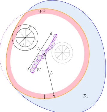
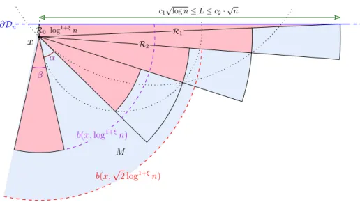
Proof. In order to bound the number of such edges, we adapt the concept of the border point introduced by Bose and Devroye [55] to bound the stabbing number of a random Delaunay trian-gulation. For B ✓ Dnand a point x 2 Dn, let kxBk := inf{kxyk : y 2 B} denote the distance
Dn 1 W L W L x C x
Figure 9: For the proof of Proposition 1818. We consider the walk from z to q in Dn, letting
W =
[
i=1
Di and W := b(w, 2 max{kzqk, !n5}),
where w denotes the centroid of the segment zq and we recall that b(x, r) denotes the closed ball centred at x of radius r. Then, for x 2 W , let C be the disc centred at x and with radius min{kxW k, kx@W k}. Partition the disc C into 8 isometric cone-shaped sectors (such that one of the separation lines is vertical, say) truncated to a radius ofp3/2times that of the outer disc (see Figure 99). We say that x is a border point if one of the 8 is a border point then there is no Delaunay edge between x and a point lying outside C, since a circle trough x and y 62 C ⇢ W \ W must entirely enclose at least one sector of C (see dotted circle in Figure 99). Thus if x has a Delaunay edge with extremity in W , then x must be a border point. The connection between border points and the number of crossing edges can be made via Euler’s relation, since it follows that a crossing edge is an edge of the (planar) subgraph of DT( ) induced by the points which either lie inside W , are border points, or lie outside of W and have a neighbour in W . Let BW denote of set of border points, EW the collection of
crossing edges, and YW the collection of points lying outside of W and having a Delaunay
neighbour within W . Then
Proposition 1616bounds |W \ |, as this is exactly the set of visited vertices. Lemmas 1919and 2020 bounding |BW| and |YW| complete the proof.
Lemma 19. For all n large enough, we have P
✓
|YW| 10 max{L0, !n5}
◆
2 exp⇣ !5/4n ⌘.
Proof. Heuristically, our proof will follow from the fact that, with high probability, a Delaunay edge away from the boundary of the domain is not long enough to span the distance between a point within the walk, and a point outside of W . Unfortunately our proof is complicated by points on the walk which are very close to the boundary of the domain, since in this case, those points might have ‘bad’ edges which are long enough to escape W . To deal with this, we will take all points in the walk that are close to the border, and imagine that every Delaunay edge touching one of these points is such a ‘bad’ edge. The total number of these edges will be bounded by the maximum degree.
To begin, we give the first case. Consider an arbitrary point x 2 W \ that is at least ! 3 n
away from the boundary of Dn. Suppose this point has a neighbour outside of W , then its
circumcircle implicitly overlaps an unconditioned region of Dn with area at least c !n3!n5 =
c !n2 (for c > 0 a constant depending on the shape of the domain). The probability that this happens for x is thus at most exp !2
n . Now note that there are at most 2n points in with
probability bounded by exp !n2 and at most 4n2 edges between points of x 2 W \ and x2 {W }c\ . By the union bound, the probability that any such edge exists is at most
(4n2) exp c !2n + exp !n2 exp⇣ !n3/2⌘. For the second case, we count the number of points within ! 3
n of the boundary of the
domain. Using standard arguments, we have that there are no more than 10 max{L, !5 n} · !n3
such points, with probability at least exp !2n . Each of these has at most edges that could exit W , where is the maximum degree of any vertex in DT( ), which is bounded in Proposition 3030. Thus, the number of such bad edges is at most 10 max{L, !5
n}!n3 · !n3 with
probability at least exp( !2
n) + exp( ! 5/4 n )
Lemma 20. For all n large enough, and universal constant C > 0, P
✓
|BW| C max{L0, !6n}
◆
2 exp⇣ !3/2n ⌘.
Proof. Since |BW| is a sum of indicator random variables, it can be bounded using (a version of)
Chernoff–Hoeffding’s method. The only slight annoyance is that the indicators 1{x2BW}, x 2 \ W are not independent. Note however that 1{x2BW} and 1{y2BW} are only dependent
if the discs used to define membership to BW for x and y intersect. There is a priori no bound
on the radius of these discs, and so we shall first discard the points x 2 lying far away from @W and W . More precisely, let BW? denote the set of border points lying within distance !n
of either W or @W , and B•
using Lemma 1010, since a point is only a border point if one of its cones is empty, and each such empty cone contains a large empty circle. So for sufficiently large n,
P |B•
W| 6= 0 exp
⇣
!n3/2⌘. (16)
Bounding |B?
W| is now easy since the amount of dependence in the family 1{x2BW}, x2 \ W
is controlled and we can use the inequality by Janson [1515, 1616]. We start by bounding the expected value E |B?
W|. Note that for a single point x 2 n, by definition the disc used to define whether
xis a border point does not intersect W and stays entirely within D, so Px(x2 BW? ) =P(x 2 BW? ) 24 exp ⇣ ⇡ 32min{kxW k, kx@W k} 2⌘ 24 exp⇣ ⇡32kxW k2⌘+ 24 exp⇣ ⇡ 32kx@W k 2⌘ (17)
and nis unconditioned in D \ W . Partition D \ W into disjoint sets as follows:
D \ W =
1
[
i=0
Ui
where Ui := {x 2 D : i kxW k < i + 1}. Similarly, the sets Ui0 := {x 2 W : i
kx@W k < i + 1} form a similar partition for W . Writing for the 2-dimensional Lebesgue measure and using (1717) above, we have
E|B? W| = E " X x2 1{x2W \W }1{x2B? W} # = Z W \W Px (x2 BW? ) (dx) 1 X i=0 Z Ui 24 exp ⇡i2/32 (dx) + 1 X i=0 Z U0 i 24 exp ⇡i2/32 (dx) = 24 1 X i=0 ( (Ui) + (Ui0)) exp ⇡i2/32 .
We may now bound (Ui)and (Ui0)as follows. Recall that W is a union of discs W = [iDi.
We clearly have that
Ui✓ 1[ j=0 x2 D : i kxDjk < i + 1 . Note that x2 D : i kxDjk < i + 1 ⇡((Rj + i + 1)2 (Rj+ i)2) (18) = ⇡(2(Rj+ i) + 1). (19)
So, assuming there are steps in the walk we get (Ui) 1 X j=0 ⇡(2(Rj+ i) + 1) = 2⇡ 1 X j=0 Rj+ ⇡(i + 1). Regarding (U0
i), note first that W is convex for it is the intersection of two convex regions. It
follows that its perimeter is bounded by 4⇡ max{kzqk, !n}, so that (Ui0) 4⇡ max{kzqk, !n}
for every i 0. It now follows easily that there exist universal constants C, C0 such that
E |B? W| = E E ⇥ |BW? | Ri, i 0 ⇤ C E 2 4 1 X j=0 Rj+ + max{kzqk, !n} 3 5 C0max{kzqk, !n}.
For the concentration, we use the fact that if kxW k, kx@W k !n then the chromatic
number of the dependence graph of the family 1{x2B?
W}is bounded by the maximum number
of points of ncontained in a disc of radius 2!n. We then have
P( 8⇡!n2) P(9x 2 D : n\ b(x, 2!n)) E " X x2 n Px(|b(x, 2!n)\ n| 8⇡!n2) # E " X x2 n P(Po(4⇡!2 n) 8⇡!n2) # exp !2n ,
for all n large enough, using the bounds for Poisson random variables we have already used in the proof of Corollary 1515. Let
W@ := x2 W max{kxW k, kx@W k} !n .
Following Equation (1818) and by the convexity of W , there exists a universal constant C00such
that P ✓ | n\ W@| C00max{L, !5n} · !n2 ! exp !2n . By Theorem 3.2 of [1515], we thus obtain for t > 0,
P(|B? W| E |BW? | + t) E exp ✓ 2t2 · | n\ W@| ◆ exp ✓ t2 8⇡ C00max{L0, !5 n} · !n4 ◆ +P⇣ 8⇡!n2⌘+P⇣| n\ W@| > C00max{L0, !n5} · !2n ⌘ exp ✓ t2 8⇡ C00max{L0, !5 n} · !n4 ◆ + 2 exp !n2 .
The result follows for n sufficiently large by choosing t := C00 L0+ !6 n .
3.4 Algorithmic complexity
Whilst we have given explicit bounds on the number of sites in n that may be accessed by
an instance of CONE-WALK, we recall that the complexity of the algorithm CONE-WALK(z, q) does not follow directly. This is because the CONE-WALKalgorithm must do a small amount
of computation at each step in order to compute the vertex which should be chosen next. We proceed by defining a random variable T (z, q), which will denote the number of operations required by CONE-WALK(z, q) in the RAM model of computation given an implementation based upon a priority queue. We conjecture that the bound for Proposition 2121 given in this section is not tight, and that the algorithmic complexity is fact be bounded by O(L0 + !n4).
Unfortunately the dependency structure in algorithms of this type makes such bounds difficult to attain.
Proposition 21. Let T (z, q) be the number of steps required by the CONE-WALKalgorithm to
compute the sequence of stoppers given by the cone-walk process between z and q along with the path generated by SIMPLE-PATH in the RAM model of computation. Let c1 > 0 be an
implementation-dependent constant, then for n large enough, we have P
✓
T (z, q) > c1· L0log !n+ !4n
◆
10 exp⇣ !n3/2⌘.
Proof. Define Mi to be the number of sites accessed during the i’th step of the algorithm. We
fix z, q and write T to denote T (z, q) for brevity. From Section 2.32.3, we know that for sufficiently large n, we may choose a constant c2 such that
T c2 1
X
i=0
⌧ilog(Mi). (20)
So that to bound T , it suffices to bound the sum in (2020). We have
P ✓ 1X i=0 ⌧ilog(Mi) 15(L0+ !n3) log(!n) ◆ P ✓ 1X i=0
⌧ilog(Mi) 3(L0+ !n3) log(!n5)| Mmax< !5n
◆ +P ✓ Mmax !5n ◆ P ✓ 1X i=0 ⌧i 3(L0+ !n3) ◆ + exp⇣ !3/2n ⌘.
The first term of which is bounded by Proposition 1616, and the bound on Mmaxcomes directly


![Figure 7: For the angle to be smaller than x given R i+1 2 [r, r + "], the stopper must fall within the dark shaded region](https://thumb-eu.123doks.com/thumbv2/123doknet/14505625.528744/17.892.318.575.144.269/figure-angle-smaller-given-stopper-fall-shaded-region.webp)