Construction and applications of discrete-time smoothing error models

September 1988 LIDS-P-1812

CONSTRUCTION AND APPLICATIONS OF

DISCRETE-TIME SMOOTHING ERROR MODELS

Martin G. Bellol Alan S. Willsky2 Bernard C. Levy3

ABST ACT

In this paper we present a unified perspective on techniques for constructing both forward and backward Markovian realizations of the error process associated with discrete-time fixed interval smoothing. Several alternate approaches are presented, each of which provides ad-ditional insight and connections with other results in linear estimation theory. In addition, two applications of such models are described. The first is a problem in the validation of an error model for a measurement system, while the second concerns the problems of updating and com-bining smoothed estimates. We also present an example of the use of our updating solution for the mapping of random fields based on sev-eral sets of data tracks.

1_{M.G. Bello was with the Laboratory for Information and Decision Systems and the Department of}

Elec-trical Engineering and Computer Science, M.I.T. He is now with The Analytic Sciences Corporation, Reading, MA. The work of this author was supported in part by the National Science Foundation under Grant ECS-8312921.

2

A.S. Willsky is with the Laboratory for Information and Decision Systems and the Department of Electri-cal Engineering and Computer Science, M.I.T., Cambridge, MA 02139. The work of this author was supported in part by the National Science Foundation under Grants ECS-8312921 and ECS-8700903, in part by the Army Research Office under Grant DAAL03-86-K-0171, and in part by Institut National de Recherche en Informatique et en Automatique during this author's sabbitical at Institut de Recherche en Informatique et Systemes Aleatoires, Renner, France.

3_{B.C. Levy was with the Laboratory for Information and Decision Systems and the Department of}

Electri-cal Engineering and Computer Science, M.I.T. He is now with the Department of ElectriElectri-cal and Com-puter Engineering, University of California at Davis, Davis, CA 95516. The work of this author was sup-ported in part by the National Science Foundation under Grants ECS-8312921 and ECS-8700903 and in part by the Army Research Office under Grant DAAL03-86-K-0171.

1. INTRODUCTION

This paper is concerned with the characterization, derivation, and application of Markovian models for the error in fixed interval smoothed estimates. Models of this type are required in several applications including two that are investigated in the last few sections of this paper. In particular we describe a model validation process in which one set of data is used to evaluate the validity of a noise model for a second set of data. We also describe the solution to estimate updating and combining problems. In the former a smoothed estimate based on one set of data is updated with a new set of data. In the latter, estimates based on separate data sets are combined. Such problems arise in the construction of maps of random fields, and we describe an application of this type in which the data sets represent non-coinci-dent and non-parallel tracks across a two-dimensional random field.

In each of these applications, smoothing error models are required, in the first prob-lem to compute the likelihood function for the validity of the specified model and in the sec-ond, to specify a model for the error in the map based on the first set of data which is then used as the basis for incorporating the new data.

In this paper we consider the construction of smoothing error models from four per-spectives:

1) the use of Martingale difference decompositions of the process noise as-sociated with the state dynamics

2) the use of the square-root information filtering framework of Bierman defined in [3], and the Dyer-McReynolds smoothed estimate recursions derived in 4

3) the use of a backward Markovian model for one-step prediction estimate errors

4) the use of Weinert and Desai's Method of Complementary Models [51

The continuous-time counterpart of approach (1) was employed in [2],[6] in order to obtain forward and backward Markov models for fixed interval smoothed estimate errors. The second approach (2), was employed by Bierman in [4] in order to derive the

Dyer-backward smoothing error model, thereby exposing the relationship between Dyer-backward smoothing error models and the Dyer-McReynolds recursions.

The continuous-time counterpart of approach (3) was carried out in an Appendix in [2]. In addition, Badawi, in [7], briefly suggests the use of approach (3) for obtaining a back-ward smoothing error model associated with discrete time problems, but does not proceed to develop the detailed results. In the development of approach (3) that follows, it will be seen that the invertibility of the one-step prediction error dynamics matrix is a necessary assump-tion for the construcassump-tion of a backward one-step predicassump-tion error model that has the same sample paths as a corresponding forward model. However, without this invertibility assump-tion, we show that approach (3) can be modified in order to construct a backward smoothing error model that satisfies the weaker requirement of having the same second order properties as a corresponding forward model.

Approaches (1), (2), and (3) described above are employed to specify backward Markovian representations for the smoothing error process. Approach (4), however, involves the use of Weinert and Desai's Method of Complementary Models [5], in order to obtain a forward Markovian representation for the smoothing error process.

In the next section we introduce some notation and perform some preliminary calcula-tions. Sections 3-6 are then devoted to the four approaches indicated previously. In Section 7 we describe the model validation application, while Section 8 is concerned with the updating and combining problems, the solution to the latter of which exposes the connection of these results to the theory of oblique projections [14]. In Section 9 we apply our updating results to a problem of mapping a random field given two data sets along non-parallel tracks across the field, and we conclude in Section 10 with some brief remarks.

2.

NOTATION AND PRELIMINARY CALCULATIONS

We consider the following state model

x(t+ 1) = F(t)x(t) + Bl(t)v(t) + B₂(t)w(t) (2.1)

y(t) = H(t)x(t) + D(t)v(t) (2.2)

where v(t) and w(t) are uncorrelated, zero-mean Gaussian white noise processes with identity covariance and are also uncorrelated with the zero-mean, Gaussian initial condition x(O). We also assume that P(O), the covariance of x(O), is positive definite, so that the state covariance P(t), which satisfies

P(t + 1) = F(t)P(t)F'(t) + B1(t)Bl'(t) + B2(t)B2'(t) (2.3)

is positive definite for all t in the interval [0,T] of interest. We also assume that D(t) is square and invertible, so that

R(t) D(t)D'(t) > 0 (2.4)

We now consider several state estimates, each of which can be viewed as a projection onto an appropriate Hilbert space of random variables. Specifically if z(t) is a zero-mean process on [O,T], let H(z) denote the Hilbert space spanned by the components of

(), 0 < r < T, let H

(z)

be the corresponding space using only Z(t), 0 < r < t while Ht(z) uses z(r), t < r < T. Also, let E(_ I H) denote the projection of a zero-mean random vector _

onto the Hilbert subspace H. With this notation, the smoothed estimate of x(t) is

the one-step-ahead predicted estimate is given by

%p(t) = E[x(t) I H- 1 (y)] (2.6)

and the filtered estimate by

xf(t) = E[x(t) I H-(y)] (2.7)

The corresponding estimation errors are denoted with tildes, e.g.,

x<(t) = x(t) - &(t) _(2.8)

Next, we recall the standard Kalman filtering formulas for x(t):

xp(t+ 1) = F(t)xp(t) + K(t)v(t) (2.9)

xp(0) = o

where v(t) is the innovations process

v(t) = y(t) - H(t)xp(t) = H(t)xp(t) +D(t)v(t) (2.10)

and the gain K(t) is given by

K(t) = [F(t)Pp(t)H'(t) + Bl(t)D'(t)] V-1(t) (2.11)

where V(t), the covariance of v(t) is given by (2.12)

and Pp(t) is the covariance of the error x(t).

Combining (2.1), (2.2), (2.9), and (2.10) we obtain a forward model for -,(t):

(t+ 1) =

rF(t)(t)

+ [G(t)

'B2(t)]

(t)( (2.13) where

r(t) = F(t) - K(t)H(t) (2.14)

G(t) = Bl(t) - K(t)D(t) = - r(t)Pp(t)H'(t)(D'(t))-_{' (2.15)}

where the last equality in (2.15) follows after some additional algebra

Note also that (2.1) can be rewritten as

x(t+1) = A(t)x(t) + _(t) (2.16)

where

A(t) =F(t) - B1(t)D-l(t)H(t) (2.17)

¢(t) = B1(t)D-1(t)y(t) + B2(t)w(t) (2.18)

From this we directly deduce

p(t+1) = A(t)xf(t) + Bl(t)D-l(t)y(t) (2.19) and

Also, from the standard formula [10]

xf(t) = Pf(t) [H'(t)R-(t)y(t) + Pp1(t) xp (2.21)

together with (2.19) we find that

F(t) = A(t)Pf(t)P;l(t) (2.22)

Finally, we note a particular decomposition of i(t) that we will find of value. Specifically, the basic property of the innovations sequence v(t) gives us an orthogonal decomposition of H(y):

H(y) = Ht ₁(y) H't() (2.23)

Writing

x(t) = 4 (t) + jx(t) (2.24)

projecting onto H(y), subtracting the result from (2.24), and using the fact that x(t), H t-l(Y), and H t(_i) are all orthogonal, we obtain

3.

BACKWARDS MARKOVIAN SMOOTHING ERROR MODELS

USING A MARTINGALE DIFFERENCE DECOMPOSITION

In this section we sketch the discrete-time counterpart of the continuous-time ap-proach, presented in [2], using martingale decompositions to derive Markovian models for the smoothing error. Throughout this section we assume that F(t), or equivalently A(t), is in-vertible (this will be true, for example, if the system matrix F(t) is inin-vertible and (F(t), B2(t))

is a reachable pair).

To begin, we take the projection of both sides of (2.16) onto H(y), subtract the result from (2.16) and use the invertibility of A(t) to obtain

x(t) = A-1(t)x(t+ 1) - A-'(t)_(t) (3.1)

where

¢(t) = ¢(t) - E[_(t) I H(y)] (3.2) This is not yet a backward Markovian model, as ¢(t) in neither white nor independent of x(t). To obtain a Markovian model, we need to obtain a backward martingale decomposi-tion of ¢(t) with respect to an appropriately chosen c-field, i.e., one consisting of all of the process y (.) and the "future" of x(.).

Specifically, let

5t = H(y)

E

Ht'( ) (3.3)

and write

where, by construction [11], ,u (t) is a discrete-time white noise sequence, independent of the future as represented by g:t. It remains then to calculate the covariance of u(t) and the expectation in (3.4). Thanks to (3.2) the independence of H(y) and HItl(g) and (2.18), we have that E [(t) I = E [(t) I = B2(t)E [w(t) I Ht.()] (3.5) u(t) = B2(t) { w(t) - E [w(t) :tJ } (3.6) As shown in Appendix A, E [wE(t) ] H+t()] = B2(t)P;1(t+ 1)Rx(t+ 1) (3.7) E [w(t)

I

H(y)] = B2(t)P 1(t + 1) x(t + 1) - x(t + 1)] (3.8)

and, of course, E [w(t)l

yt]

is simply the sum of these, so that

u(t)= B2(t) [w(t) - B'(t)P'(t + 1)(t + 1)] (3.9)

Thus we have the backward Markovian model

(t)= A- (t) -B 2(t)FB; (t (t+ 1)] (t + 1)- A- (t),(t) (3.10)

where, from (3.6) - (3.9), we have that the covariance of the white noise u (t) is

4. BACKWARDS MARKOVIAN SMOOTHING ERROR MODELS FROM

SQUARE-ROOT INFORMATION FILTERING

In this section we make explicit the connection between the backward model (3.9) -(3.11) derived in the preceding section and square-root information filtering [3,4] and in par-ticular the Dyer-McReynolds backward smoothing error covariance recursion.

We begin by recalling the filtering and prediction steps of square-root information fil-tering. Consider the problem of ex)ti,,,,i,,, satisfying (2.16) - (2.18) given y(t) given by (2.2). Let

[Pp(t)]-l = Sp(t)Sp(t) (4.1)

[Pf(t)]-' = Sj(t)Sf(t) (4.2)

P(t) = Sp(t)xp(t) (4.3)

Zf(t) = Sf(t)xf(t) (4.4)

Given Sp(t), z_(t), the filtering steps then consists of constructing of a Householder transformation T1(t) that produces the zero block in the following equation and

conse-quently also yields Sf(t) and zf(t) as well

SP(t) zp(t)[Sf(t) ZfI(t)1

T1(t) --- =-- (4.5)

D-1(t)H(t), D-1(t)y(t) ] :

Given S f(t), z f(t) the prediction step consists of constructing a Householder trans-formation T2(t) to produce the indicated zero blocks (and consequently the other

quanti-ties indicated) on the right-hand side of the following

T₂(t) .

- Sf(t)A-l(t)B2(t)

Sf(t)A-l(t)

zf(t) + Sf(t)A-l(t)B1(t)D-l(t)y(t)]

Sw(t S(t + 1) r(t) (4.6)

_ O Sp(t + 1) Zp(t + 1) J

where the top blocks in these matrices have m rows, where dim (w) = m. Also, the quanti-ties in the top block row on the right-hand side of (4.6) can be given precise statistical in-terpretations related to the best filtered estimate of the process noise w(t).

For our purposes the key point is that Bierman [3,4] uses these results to derive the following algorithm for computing the smoothed estimate

x(t)

= A-l(t) [L(t + 1) - Bl(t)D-1(t)y(t) - B2(t) s(t)] (4.7)

ws(t)

= SW1(t) [(t) - Swx(t+1)iX(t+1)] (4.8)

with

ix(T) = Sf'(T) Z (T) (4.9)

where w_(t) is the smoothed estimate of w(t) . Bierman also shows that x(t) satisfies the following backward model:

x(t) = A-l(t)[(I + L(t)Swx(t + 1))x(t + 1) - B1(t)D-l(t)y(t) (4.10) -L(t)r(t) + L(t)w(t)]

where

L(t) = B2(t)Sw(t)l (4.11)

and

w(t) = - Sw(t)w(t) - S,,(t + 1) x(t + 1) + r(t) (4.12)

A byproduct of the square-root algorithm is that wo(t) is a zero-mean white noise process independent of H( y) and with identity covariance.

Combining (4.7), (4.8) to obtain a single backward equation for ,(t) and subtract-ing from (4.10) yields the desired backward model for x(t):

x(t) = A(t) t) [I + L(t)Swx(t + 1)] i(t + 1) + A-'(t)L(t)wo(t) (4.13)

from which we can also derive the Dyer-McReynolds smoothing covariance recursion:

Ps(t) = A-'(t) [I + L(t)Sx(t + 1)] Ps(t + 1) [I + L(t)Swx(t + 1)1' [A'(t)]-1

+ A-l(t)L(t)L'(t) [A'(t)]-1 (4.14)

Finally, using an argument analogous to that on pp. 220-221 of [3] we can show the first equality of the following

A-1(t) [I + L(t)Swx(t + 1)] = Pp(t)A'(t)P;3 (t + 1)

where the second equality follows from (2.20). Thus

L(t)S,,(t + 1) = - B2(t)BE(t)Pp1(t + 1) (4.16)

Also, from (4.8) and (4.12) we see that

L(t)ro(t) = - B2(t) [ [w(t) - ws(t)] + Sl(t)Swx(t+ 1) (t+ 1)] (4.17)

Using (4.16) and the expression for w,(t) in (3.8), and comparing to (4.17), we see that

L(t)w(t) = -8(t) (4.18)

That is, the model (4.13) is identical to that derived in Section 3, although we now have made explicit contact with quantities arising in square-root algorithms.

5. BACKWARDS SMOOTHING ERROR MODELS FROM BACKWARDS

PREDICTION ERROR MODELS

In this section, a backwards counterpart to the forward Markovian model (2.13) for one-step prediction errors is used together with (2.25), in order to obtain a backwards Markovian representation for the smoothing error process. The approach presented here ex-poses the intimate connection between the structure of backward smoothing and one-step prediction estimate error models. In addition, towards the end of this section it is shown how the approach here can be applied to the construction of backward smoothing error modeis in the case when r (t) is singular.

Suppose that

r

(t) is invertible. Then, using results in [8], we obtain the following backward Markovian counterpart of (2.13):

&(t) = r-'(t)

{I

- [G(t)G'(t) + B2(t)B2(t)] pl (t + 1)} ,(t + 1)

0),, .,,[r(t)

-st

(5.1)

r- (t)

[G(t) B2(t)]0(t) where

L(t)

=

Lw

(t) l

BP'2(t + 1)xp(t + 1)

(5.2) is a white noise process independent of the future of xSp(.) and with covariance

Cov

7I(t))

=

_I-

LB'(t).

_{P;'(t + 1) [G(t) B}

Some algebra (using (2.13) and its associated Lyapunov equation) yields the following equivalent forms for (5.1) and (5.2):

xp(t) N=(t) t)(t+ 1)

+ [Pp(t)H'(t)(D'(t))-1

_ r- (t)B2(t)]

(t)

()

LQ(t)

where N(t) = Pp(t)F'(t)Pl'(t+ 1) and Q(t) w(t) B(t)J ap(t)B A M(t) (t) (5.6)

Using (2.10) and (2.15) we find that

a(t) = D-l(t)v(t) (5.7)

Also, from (5.5), (5.6) and standard linear estimation results we can write

,B(t) = -B'2(t) (r'(t))-'Pp~(t) E[x(t) I v(t)] + y(t)

(5.8) = - B'(t) (r (t))-1H' (t ) V -1( t)v( t) + y(t)

where y (t) is independent of v (t), with

E

L(t)y'(t)]

= I + B'(t)(r'(t))- P'l(t)Pf(t)Pp;(t)(F(t))- B2(t)

(5.9) = I + B'2(t) (r'(t))- [Pp'(t) - H'(t) V-l(t) H(t)] F-I(t)B2(t)

where we have used the standard formula

Pf(t) = Pp(t) - Pp(t) H'(t) V-'(t) H(t) Pp(t) (5.10) Performing some algebra (again using (2.15), (2.13), and its (Lyapunov equation) and summarizing, we now have the following backward Markovian model for ip(t):

ip(t) = N(t) x,(t + 1) - N(t) B2(t) y(t)

(5.11)

+ N(t) [F(t)Pp(t)H'(t)R-1(t) + B2(t)B'2(t)(F'(t))-1H'(t)V-1(t)] v(t)

where y(t) and v(t) are independent white noise processes with covariances given by (5.9) and V(t), respectively.

Note that the independence of y (t) and v (t) implies the orthogonality of y (t) and all of H(y). From this fact, it is quite straightforward to obtain a backward model for the smoothing error, simply by projecting (5.i 1) onto H(.) and subtracting from (5.11). This yields the desired model

x(t) = N(t)#(t + 1) - N(t)B2(t)y(t) (5.12)

Some further algebra then yields that

Finally, let us comment on the extension of these results to the case when either F (t) or Pp(t) are not invertible. Using the results of [81 one can see that the invertibility of

r

(t) is necessary for the construction of a backward model for i p (and ultimately for x) that has exactly the same sample paths; however the invertibility of Pp is not neces-sary. If Pp is singular, the corresponding results are obtained by noting that

E[x,(t) I Ht l1p)] = Pp(t)r'(t)P(t + 1)p(t + 1) (5.14)

where "#" denotes the Moore-Penrose pseudo-inverse. If F(t) is invertible, the analysis of this section can be carried out starting from (5.2) - (5.4) with the sole change being that now

N(t) = Pp(t)F'(t)iP(t+ 1) (5.15)

If F(t) is singular, we can still obtain a backward model that has the same second-order statistics as i . Specifically, thanks to (5.14), we can write

I(t) = N(t):x(t+1) + 6(t) (5.16)

where N(t) is given by (5.15) and 6 (t) is a white noise process independent of the future of ;j(t). Furthermore, by construction B (t) is independent of H'+l(_) and, thanks to

(5.16) it is also independent of H- 1(.). Thus we can write

8(t) = EW(t) I v(t)] + _(t) (5.17)

where _ (t) is a white noise process independent of the future of x and of H(y). Thus, in the same manner as used previously, we obtain the backward model

x(t) = N(t)R(t) + s(t) (5.18)

6. CONSTRUCTION OF A FORWARD SMOOTHING ERROR MODEL

In this section we use the method of complementary models [5,6,12] to derive a for-ward smoothing error model that requires neither the invertibility of F (t) or of P(O). To be-gin, recall the form of the state model given by (2.16) - (2.18), and consider the following processes

x* (t+ 1) = A(t)x'(t) + B2(t)w(t) (6.1)

y'(t) = H(t)x'(t) + D(t)v(t) (6.2)

with

x*(O) = x(O) (6.3)

From (2.2), (2.16), (2.18), and (6.1) - (6.3) we can deduce that for t > 0 t-1 x (t) = x(t) - ( A(t,T+ 1)B₁(T)D-l(r)y(r) (6.4)

T=0

y*(O) = y(O) and for t > 0 t-1

y(t = y(t)- H(t)DA(t, r + 1)Bl(r)D-l()y(r) (6.5)

0=0

where DA(., .) is the transition matrix associated with A. From (6.5) we see that H (y) = H (y*) and then from (6.4) that

Note that the model (6.1), (6.2) has uncorrelated process and measurement noises. In the following development we write

x(0) = TE 6 _(6.7)

where E is a random vector with identity covariance. The method of complementary

models consists of identifying the space Yo, where

H() H( H()

E

H ) = H(y*)

E

Yc (6.8) Then X(t) = E [X*(t) I Yc] (6.9) Results in [5,6,12] yield Y, = H(U) E H(Z) (6.10) where =

-

TEA' (O0);(0) - TcH' (0)[D'(0)]-lv(0) (6.11) z(t) = _{- B(t))_(t) + w(t)} (6.12) and . (t) satisfies the backward equation

A(t) = A'(t + 1)A(t + 1) + H'(t + 1) [D'(t + 1)]-'v(t + 1) (6.13)

A(T) = 0 (6.14)

To obtain a forward model for i we first obtain an alternate basis for Y , namely

= _- EL I H(z)] (6.15)

Note that ip and Vz(.) are uncorrelated and v7(t) is a white noise process, representing

the innovations process associated with the Kalman filter for the reverse-time model (6.12) - (6.14). These quantities and their covariances can be generated using standard Kalman filtering formulas (applied backward in time). Specifically, let

=E(t)

= E ._(t) I Hf(z)] (6.17)

p(t) = E A(t) I H1(z)] (6.18)

with 2

f(t) and &(t) denoting the corresponding errors and Of(t) and

ep(t)

the corresponding error covariances. Then

g(t)

= [I -

ef(t)B

2(t)B2(t)] p(t) + Of(t)B 2(t)W(t) (6.19)

~p(t) = A'(t + 1)A(t + 1) + H'(t + 1) [D'(t + 1)]-lv(t + 1) (6.20) with

f(T) = 0 (6.21)

where

Of(t) = p(t) - EO(t)B2(t) [B'(t) Ep(t)B2(t) + I]-'lB(t)

EO(t)

(6.22)

op(t) = A'(t + 1) Of(t + 1)A(t + 1) + H'(t + 1)R-l(t + 1)H(t + 1) (6.23) with

Of(T) = 0 (6.24)

Thus, from (6.11), (6.12), (6.15), and (6.16)

and, using (6.22), (6.23)

E[_p] - I + TIA'(0) 8f(0)A(O)TE + TH'(0)R-'(O)H(O)T, (6.27)

E[v(t) v(t)] = I + B'(t) ep(t)B2(t) (6.28)

We are now in a position to compute

(t)

=

E [ (t) ]

E [

_']-'

+ EN

E[

[(r)V.(rT)] E [(v)E(T)Y 4(v) (6.29)

From (6.1), (6.19), (6.20), and some algebra we find that

E [x*(t)1]

=

(A(t, O)TE

t-1

+ ) ,^A(t, r + 1)B2()B2(r) Ef(r)IE(O, r)A(O)TE '-0 - 'I(t, O)TE (6.30) where

1I

t=

T _(6.31) /DE(t, T ) {(t) : I _6-4t t=r_{= r}

with

E(t) = [I - Of(t)B2(t)B'(t)] A'(t + 1) (6.33)

and {G(t- 1) .. G(t) t > r DG(t, T) I t = r (6.34) with G(t) = [I - B.(t)B'(t)Of(t)1 A(t) (6.35) Also 0 tr>t

E

L*

(t)(v)] =

I

DGo(t, r + 1)B2(r)

T < t

(6.36)

Combining (6.27) - (6.36) we obtain the following forward model for g(t):

(t+ 1) = G(t)(t) + B2(t) [I + B(t) ep(t)B2(t)]1 ~(t) (6.37)

with

7.

MODEL VALIDATION USING TWO MEASUREMENT SETS

In this section we describe and develop one important application of smoothing error models, namely to a particular problem of model validation. Specifically we consider a prob-lem in which two measurement systems are used to provide information about the same physical process. Associated with each system we have a dynamic model describing the error and noise sources in the system. One of these models is assumed to have been validated, and the objective is to evaluate the validity of the model for the other measurement system. A problem of the type just described arises in the mapping of earth's gravitational field [16]. A wide variety of sensors, sensitive to different ranges of spatial wavelengths, is available for this application. For example, satellite orbit data provides information on very long wavelength variations, satellite altimetry data is sensitive to intermediate wavelengths, and ship-borne gravimetry data yields information at still shorter wavelengths. An overall map of the gravity field is then obtained by combining such sources of information.

Maps of this type are used in a variety of contexts such as in aiding navigation sys-tems on ships, and in such a context it is necessary to have statistical models for the map er-rors in order to allow one to make predictions concerning navigation system accuracy. Validating such models is of great importance in such an application, and one way in which to design an evaluation procedure for such a model is to obtain two sets of "measurements" for the same gravity-field-related quantity: one set derived from map information and a sec-ond set derived from a different data set, the error model for which has been adequately de-termined. Using this information one would like to construct likelihood functions related to the parameters and validity of the map error model. It is this problem that we now abstract and study.

Consider the following process that is under observation

o(t+ 1) = Fo(t)Xo(t) + Bo(t)wo(t) (7.1)

Suppose that we have two sets of measurements

yi(t) = z(t) + ni(t) , i= 1,2 (7.3) where the noise model for nl(t) is known:

xl(t+ 1) = Fl(t)xl(t) + Bl(t)wl(t) (7.4)

nl(t) = Hl(t)xl(t) + Dl(t)wl(t) (7.5)

while the corresponding model for n2(t) is parameterized by a vector A:

x2(t+1) = F2(t;A)x2(t) + B2(t;A)w2(t) (7.6)

n2(t) = H2(t;A_)x2(t) + D2(t;A)w2(t) (7.7)

where xi(O), i=0,1,2, wi(t), i=0,1,2 are mutually independent zero-mean and Gaussian, with

E [x(O)x(O)] = Pi(O0), i= 0, 1 E [xz(0)~x(0)] = P2(0; A) (7.8)

E [i(t)y(r)] = Qi(t)6t,r, i = 0, 1 E [_(t)w(r)] = Q2(t;A) 6t,r (7.9)

The objective is to compute the likelihood function

p(Y1, Y2;

A)

(7.10)

where

This can then be used for model validation and parameter estimation. What we demon-strate now is the central role played by smoothing error models in the computation of (7.10). Specifically, note that

P(Yl, Y; = P(Y)(Y I Y1; A)

= P(Y1)P(Y2;A (7.12)

where

>=

[

(0o),. , y_(T)] (7.13)

y2(t) 2(t) -(t) - Yl;Alj (7.14)

= ls(t) + n2(t) (7.15)

where ~l,(t) is the error in estimating z(t) given Y1. A Markovian model for this

er-ror can be constructed using the methods in Section 3-6 based on a state model con-sisting of (7.1) - (7.5) (using only yl(t) in (7.3)). The computation of p(Y2;A) is then a standard problem. Specifically, if we have constructed a forward model for the smoothing error Z1l(.) , we now have an overall forward model consisting of this

for-ward error model, (7.15), and (7.6), (7.7). Standard Kalman filter-based methods then provide the required recursions for computing p(_2; A). If we have constructed a backward model for _,(.), we first obtain a backward Markovian model correspond-ing to (7.6), (7.7) (uscorrespond-ing the method in [8]) and then apply Kalman filter recursions in reverse time.

8.

UPDATING AND COMBINING OF SMOOTHED ESTIMATES

In this section we describe the discrete-time counterparts of the continuous-time re-sults on updating and combining estimates developed in [1,2]. We also present some new in-sights to clarify the structure of the solution by making use of the idea of oblique projections employed in [13] to solve decentralized filtering problems. As discussed in [1,2], the prob-lem considered here is motivated by spatial data assimilation probprob-lems such as combining gravitational maps based on different data sets and updating such maps as new measure-ments become available. In the next section we give an example indicating the applicability of these discrete-time results to a particular non-trivial measurement geometry, namely data sets along non-parallel tracks across a random field.

Let x(t), given by (2.1) be the process to be estimated, and suppose that two sets of measurements are available:

yi(t) = Hi(t)x(t) + v1(t) , i = 1,2 (8.1)

where w(t), vl (t), v2(t) are mutually independent, and

E[wi(t)f(t)] = Ri(t)6t.r (8.2)

The smoothed estimates based on yi alone or on (Yl, Y2) together are, respectively, given by

xi,(t) = E [I(t)

I

H(yi)] , i= 1,2 (8.3)

x(t) = E [x(t)

I

H(yl,y2)] (8.4)

The updating problem is concerned with the computation of j in terms of x1, and Y2 i.e., with updating xis given the new data Y2. The following elementary Hilbert space argument shows that this is possible and leads to an algorithm directly involving the use of a smoothing error model.

To begin, we define the error process

y2(t) = y2(t) - E [y2(t) I H(yl)] (8.5)

Then we have the following orthogonal sum decomposition

H(y1,Y 2) = H(yl)

E

H(y2) (8.6)

If we then project x(t) onto both sides of (8.6) we obtain

x<(t) = x1,(t) + E [x(t) H(y₂)] (8.7)

However, x(t) = ls (t) + X₁s (t), and it is not difficult to check that

y2(t) = H2(t)Xls(t) + Y2(t) (8.8)

so that x1l(t) is orthogonal H(02). Thus

x<(t) = xls(t) + E [.1s(t)

I

H(y2)] (8.9)

which represents the solution to the updating problem. Specifically, using results in Sections 3-6, we can construct Markov models for x1s(t) which, when combined with

(8.8), allow us to use standard smoothing algorithms to compute E [xl,(t) I H(y2)].

The combining problem is concerned with the computation of in terms of xl, and xs. To solve this, let us first note the counterparts of (8.5), (8.8), and (8.9) with 1 and 2 reversed:

(t y₁(t) -= - E [y [y(t) H(y₂)]

(8.10) = H1(t)x2s(t) + vl(t)

Adding (8.9) and (8.11) and subtracting x(t) yields

is(t)

= xlS(t) + X2s(t) + {E [kl(t) I H(y:2)] + E [x2 (t)

I

H(_x)] - x(t) } (8.12)

To show that this is an abstract solution to the combining problem we must verify that the bracketed term in (8.12) is a function of x1s and x_2s alone. In [1,2], in the con-tinuous-time context, this is demonstrated by purely algebraic techniques which also yield two-filter algorithms for computing the bracketed term from 1s, and x2,.

Alge-braic techniques also form the basis for the discrete-time solutions presented in

[17,18]. In this section we follow a different path based on the theory of oblique pro-jections that also provides us with deeper insight into the geometric nature of the solu-tion and of the role played by smoothing error models in computing these oblique pro-jections.

To begin, let us preview the final answers. Specifically, let L1 and L2 denote

the linear operators such that

E [2s,(.) I H(:1)] = Li(:1) (8.13a)

E

i,(.) I H(y2)] = L2(_2) (8.13b)

What we will show is that the smoothed estimate x can be expressed as follows

xS(.) = L₁(y1) + L2(y2) (8.14)

Assuming this is true and using (8.8), (8.10), and (8.12)-(8.14) we find that

What (8.15) says is the following. Recall that the computations in (8.13a) and (8.13b) are standard smoothing problems, thanks to the existence of Markov models for x1s and x2s. Thus L1 and L2 can be implemented in a variety of ways such as the

two-fil-ter form for the optimal smoother. Then, according to (8.15) x is computed from X1s and ~xs by adding the two and subtracting the outputs of the algorithms implementing L1 and L2 when these have H1x2s and H2 1ls respectively, as inputs.

What remains now is to demonstrate the validity of (8.14). We begin by recall-ing the oblique projection result stated in [6]. Let G be a closed subspace of a Hilbert space H with the following direct, but not necessarily orthogonal, decomposition

G = M1 + M2 (8.16)

Then for any a E H, the projection of a onto G, denoted by P [a I HI can be uniquely expressed as

P [a I H = al +a 2 , ai EMi (8.17)

The a i are the oblique projections of a, uniquely determined by the orthogonality condi-tions

< P[a

l

li] - ai, t > = 0 for all e 1Mi, i=1,2 (8.18)

where <., · > is the inner product on H, and Mi is defined as

Ii = span {B- P[ ,B Mj] I P E Mi}, where j # i (8.19)

In our context, G = H(yl, Y2), Mi = H(yi), Mi = H(yi), and a = x(t). Then

where K1 and K2 are the oblique projection operators. Also, in this context

P [a I Mi] = E [x(t) I H(yi)] = E [.~j(t) I H(yi)] = Li(yi) (8.21)

where j * i and the second equality follows from the orthogonality of Rj and yi. Thus in our case the orthogonality condition (8.18) becomes

[Li(y) - Ki(yi)] _L H(yi) (8.22) and the problem is to find the (unique) operator Ki that satisfies (8.22). We now show that the choice is

Ki = L, (8.23)

Indeed if we make this choice and use (8.8), (8.10) we find that (8.22) reduces to

- Li(H js) _I_ H(-y) (8.24)

which is valid thanks to the orthogonality of xis and Yi.

9.

A MAP UPDATING EXAMPLE

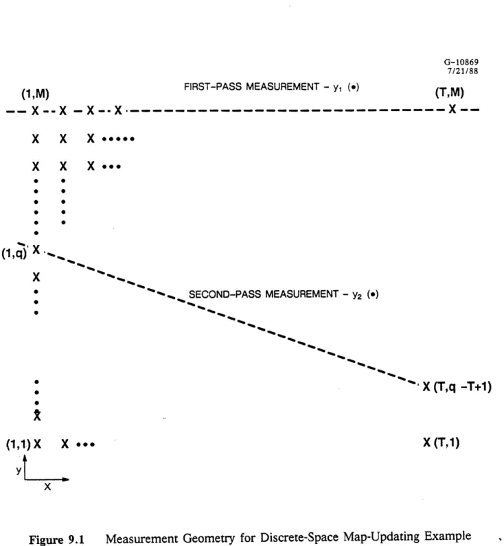
In this section we consider a discrete space map-updating problem corresponding to a measurement geometry with non-parallel measurement tracks through a scalar, separable, stationary, random field. As will become clear, our approach can be applied to a large class of discrete space mapping problems.

Let f(i,j) , i=1,..., T, j=1,..., M denote a two-dimensional zero-mean random field with correlation function

E [f(m + i, n +j) f(m, n)] A- R(i,j) = pa il Ijl (9.1) For simplicity let us consider a problem in which each data set consists of a single track of data across the field. Specifically the two data sets are defined by

y1(t) = f(t,M) + vl(t) , t = 1,...,T (9.2)

y2(t) = f(t,q-t+1) + v2(t) , t = 1,...,T (9.3)

where v1(.) , v2(.) are independent, zero mean white noise processes with

E[v?(t)] = ri , i=1,2 (9.4)

The measurement geometry is depicted in Fig. 9.1. Again for simplicity we assume that

T < q < M (9.5)

so that y2(t) is defined for t = 1,...,T, i.e., so that the second track of data is a

G-10869 7/21/88 (1,M) FIRST-PASS MEASUREMENT - y, (.) (T,M)

--

X--X

X .…---.---

X

-

--

- - - - ---

X

X X X .----X X X .. X -SECOND-PASS MEASUREMENT - Y2 (-)

-

-

(T,q -T+1)

(1,1) X X *- X (T,1)

Yl

x

We now demonstrate that this problem can be cast in the framework described in the preceding sections. The state model we use, which is essentially the same as that used in [14], describes the evolution of the set of values {f(t,j), j=l,..., M } as t

increases from 1 to T. Specifically, let

z(t) = [f(t,M), ... , f(t, 1)]' (9.6) Then a state model for our field is

x(t+1) = Fx(t) + Bw(t) (9.7a)

with

z(t) = Cx(t) (9.7b)

where x(t) and w_(t) are M-dimensional, w(t) is white noise with identity covariance, and

F = aI (9.8a) B = [p (1-a2)]1/2 I (9.8b) E [x(O)x'(0)] = P = pI (9.8c) and p~i-1 if j= 1 Ci= i-ji (i - 2)1/2 if 1 < j

< i

(9.8d) O otherwise

From (9.2), (9.3), (9.6), and (9.8) we also have

y1(t) = Hlx(t) + v1(t) (9.9)

where H1 = [1,0,...,0]C = [1,0,...,0] (9.11) (m - q + t)th - position H2(t) = [0, ... , 0, 1, O,..., O0 C (9.12) [ [M+t-q-I , M+t-q-2 (1 _2)1/2... (1 _- 2)1/2 0, ... , 0]

Note that our random field has a separable covariance. Since the first measurement set is along one of the directions of separability, we obtain a time-invariant model (9.9). The second measurement set, however, is not along such a direction, and the resulting model is time-varying.

Our problem is now set up exactly in the form used in the preceding section. For example, the map updating solution is given by

jz(t)

= Cx(t) (9.13)

where

x(t)

=

x_,(t)

+ E [,s(t) I H(Y2)] (9.14)

Note that the special structure of the state model (9.7), (9.8) leads to considerable sim-plification. Specifically, the components of

x(t) = [x (t), ... ,xM(t)] (9.15) are independent. Since y1(t) only measures the first component of x(t),

and thus the smoothing error model for j Is (t) consists of the original models for X2(t),..., X t(t) and the scalar smoothing error model for xl(t). Some algebra [6] then

yields the following model

xl,(t + 1) = F(t)xls(t) + B(t),w(t) (9.17) Y2(t) = y2(t) - H2(t)xls(t)

= H2(t)Xls(t) + v2(t) (9.18)

where

F(t) = diag (a(t), a I) (9.19a)

B(t) = diag (b(t), [p(l -a 2)]1/2 I) (9.19b)

where

a(t) = a [1 - p(l -a 2) P1b(t)] (9.20a) b(t) = {p(1 -a 2_{) [1 - p(1 - a}2_{) Plb(t)] }1/2 (9.20b)}

and Plb(t) satisfies the backward recursion

Plbt)

a

2P1b(t+1) +

1/r

1

(9.21a)

p(1 -a 2) [a2Plb(t+l) + 1/rl] + 1 with

Plb(T) = 0 (9.21b)

Finally, the initial covariance for (9.17) is

E j,(1)>S,(1>)] = diag (P(l), p, ... , p) (9.22a)

where

Note also that the triangular structure of C and hence of H2(t) also implies

consider-able simplification for the solution to the smoothing problem for (9.17), (9.18)

(see [6]). All of this indicates that particular efficiencies may be obtained by careful choice of state representations that take advantage of the geometry of the measure-ments and the correlation structure of the underlying random field. Note also that the method developed in this section can be immediately extended to correlation models of the form

R(i,j) = . A(i) i ( ) (9.23)

where Op(-) and ,p(.) are one-dimensional correlation functions realizable as the correlation of the output of finite-dimensional linear systems. Representations of this type can be used to approximate correlation structures of a large class of random

10.

CONCLUSIONS

In this paper we have considered the construction and application of Markovian mod-els for the error in fixed-interval smoothed estimates. In particular we have described three alternate approaches to the construction of backward models, each of which provides addi-tional insight and connection to other results in linear estimation. In addition, the third of these methods makes clear the necessity of the invertibility of the one-step prediction transi-tion matrix for the constructransi-tion of a backward model with identical sample paths. On the other hand, the forward model developed using the method of complementary models has no

such requirement.

We have also described two applications in which smoothing error models play a cen-tral role, namely a particular model validation problem and the problems of map updating and combining. In the case of the combining of smoothed estimates we have exposed the connection of the problem to the theory of oblique projections. We have also presented a problem of updating the map of a 2-D random field given data along non-parallel tracks. In this case, the non-parallelism manifests itself in the nonstationarity of the resulting 1-D mod-els. Also, by judicious choice of realization, the computations required in constructing the smoothing error model and in the subsequent updating operation can be greatly simplified.

APPENDIX A

In this appendix we verify (3.7) and (3.8). To demonstrate the validity of (3.7) we must show that

E [w(t)) - B'2(t)Pp t + ()(t 0, 1, 2,... (A. 1)

Fr'om (2.10), (2.13), and (2.25) we can write the following explicit formula for n s (t):

x(t) =

xp(t)

- Pp(t)

1r

(T, t) H'(r) V-(r)v(T) (A.2)

t=t

where Or (.,.) is the transition matrix associated with r(t). Using (A.2), (2.10), and (2.13) we can then make the following computations:

E [(t)x(t +)] = B'2(t) <Dr(t *, t + 1) T

B(t) (,t+ 1) () V()

H()

r(,t+)

P(t+)

(A.3) r=t+A E [x,(t + 1)g(t +4)] = Pp(t + 1)

Ir(t

+A, t + 1) T -Pp(t+ 1) Z I

r(r,t+

1) H'(r) V-1 (r) H(r) Or(r, t+ ) Pp(t +.) (A.4) r = t +.A

To verify (3.8), we note that from (2.23) we have that

E [w(t) I H(y)] = E [w(t)

I

H;.1()] (A.5)

This, together with (2.10) and (2.13), allows us to obtain the formula

E [w(t) I H(y)] = B'(t)

[

r (r, t + 1) H'(r) V- (r) v(r)]

(A.6)

APPENDIX B

To derive the covariance of _ (t) in (5.18) we begin by noting the following equalities:

x,(t) = f(t) - E [f(t) I Ht+l(1

(]

(B.1)

,(t) = ip(t) - E [ip(t) I H (v)] (B.2)

E [x(t) I H,+(_)] = E [.p(t) I Hiv(_] (B.3)

E[ i,(t) I H~+ (D] = N(t)Ei[p(t + 1) I Hal(Z)] (B.4)

where (B.4) follows from (5.16). Substituting these into (5.18) (with (B.2) evaluated at t+1) we obtain

~(t) = E(t) - N(t) xp (t + 1) (B.5) Using (2.17), (2.19) we then obtain

E [_(t)' (t)] = Pf(t) - L(t) S(t) - S(t) L(t) + L(t) S(t) L(t)

(B.6)

where

L(t) = Pp(t) Pp(t) (B.7)

APPENDIX C

In this appendix we demonstrate the validity of (8.14) without reference to oblique projections. To begin, define the operators

xiS = Ni(yi) (C. 1)

E [Yi I H(y)] = _{Sij=() (C.2)}

Then using (8.13a), (C.1), and (C.2), we can rewrite (8.11) xc = N2(Y2) + L1 (y1)

= N2(Y2) + Ll(yl - S12(Y2))

= Ll(y1) + [N2 - L1S12] (Y2) (C.3)

Now the defining requirement for L2 implies that

[ - L2( 2)]

I

H(y2) (C.4) Writing x = x + xx and using (C.3) and the expression

Y2 = Y2 - S21 (Y1) (C.5)

we find that (C.4) becomes

+ [L1+ L2S2 1] (Y1) + [N2 - L1S1 2 - L2] (Y2)}

i

H(Y2) (C.6)

Since x and Yl, are both orthogonal to H(y2) but Y2 is not, we must have

L2 = N2 - L1S12 (C.7)

REFERENCES

1. Willsky, A.S. and Bello, M.G., et.al. "Combining and Updating of Local Estimates and Regional Maps Along Sets of One-Dimensional Tracks," IEEE Transactions on Automatic Control, Vol. AC-27, pp. 799-813, August 1982.

2. Bello, M.G., and Willsky, A.S., et.al. "Smoothing Error Dynamics and their Use in the Solution of Smoothing and Mapping Problems," IEEE Transactions on Information The-ory, Vol. IT-32, pn. 483-495, July 1986Q

3. Bierman, G.J. Factorization Methods for Discrete Sequential Estimation Academic Press, New York, 1977.

4. Bierman, G.J. "Sequential Square Root Filtering and Smoothing of Discrete Linear Systems," Automatica, Vol. 10, pp. 147-458, 1974.

5. Weinert, H.L. and Desai, V.B., "On Complementary Models and Fixed-Interval Smoothing," IEEE Transactions on Automatic Control, Vol. AC-26, pp. 863-867, August 1981.

6. Bello, M.G., "Centralized and Decentralized Map-Updating and Terrain Masking Analysis," Ph.D. Dissertation, Department of Electrical Engineering and Computer Sci-ence, M.I.T., Cambridge, Mass, August 1981.

7. Badawi, F., "Structures and Algorithms in Stochastic Realization Theory and the Smoothing Problem," Ph.D. Thesis, Department of Mathematics, University of Ken-tucky, Lexington, KenKen-tucky, January 1980.

8. Verghese, T., and Kailath, T., "A Further Note on on Backward Markovian Models," IEEE Transactions on Information Theory, Vol. IT-25, pp. 121-124, January 1979. 9. Desai, U.B. and Kiaei, S. "A Stochastic Realization Approach to Reduced-Order

Hier-archical Estimation," 24-th IEEE Conference on Decision and Control, Vol. 1, pp. 416-421.

10. Jazwinski, A.H. "Stochastic Processes and Filtering Theory," Academic Press, New' York, 1970.

11. Segal, A., "Stochastic Processes in Estimation Theory", IEEE Transactions on Informa-tion Theory, Vol. IT-22, pp. 275-286, 1976.

12. Adams, M.B., Willsky, A.S., and Levy, B.C., "Linear Estimation of Boundary Value Stochastic Processes, Parts I and II," IEEE Trans. on Automatic Control, Vol. AC-29, No. 7, pp. 803-821, Sept. 1984.

13. Desai, U.B. and Kiaei, S. "A Stochastic Realization Approach to Reduced-Order Hier-archical Estimation," 24-th IEEE Conference on Decision and Control, Vol. 1, pp. 416-421.

14. Powell, S., and Silverman, L., "Modeling of Two-Dimensional Covariance Functions with Application to Image Restoration," IEEE Transactions on Automatic Control, Vol. AC-19, pp. 8-12, February 1974.

15. Woods, J. and Radewan, C., "Kalman Filtering in Two Dimensions," IEEE Transactions on Information Theory, Vol. IT-23, pp. 473-482, 1977.

16. Nash, R. and Jordan, S., "Statistical Geodesy, An Engineering Perspective," Proceed-ings of the IEEE, Vol. 66, pp. 532-550, 1978.

17. Bierman, G.J. and Belzer, M.R., "A Decentralized Square Root Information Filter/ Smoother", Proceedings of the 24th Conference on Decision and Control, Ft. Lauderdale, FL, December 1985, pp. 1902-1905.

18. Watanabe, Keigo, "Decentralized Two-Filter Smoothing Algorithms in Discrete-Time Systems", Int. J. Central, Vol. 44, No. 1, pp. 49-63.