Essays in household finance and monetary policy transmission

(1)

U

NIVERSITÀ DELLA

S

VIZZERA ITALIANA

D

OCTORAL

D

ISSERTATION

Essays in Household Finance and

Monetary Policy Transmission

Author:

Virginia GIANINAZZI

Supervisor:

Prof. Alberto PLAZZI

A dissertation submitted in fulfillment of the requirements for the degree of

PhD in Economics SFI PhD in Finance in the Institute of Finance Faculty of Economics Dissertation Committee:

Prof. Francesco FRANZONI, Università della Svizzera italiana

Prof. Loriana PELIZZON, Goethe University

Prof. Alberto PLAZZI, Università della Svizzera italiana

Prof. Marti SUBRAHMANYAM, NYU Stern School of Business

(2)

(3)

iii

Abstract

The chapters in my dissertation use novel empirical settings to contribute new in-sights to two fundamental questions in finance: how households make financial de-cisions and how market prices react to uninformative demand shocks.

In the first chapter, Reference Points in Refinancing Decisions, I exploit the unique de-sign of mortgages in the UK to study how households make mortgage refinancing decisions. Several recent papers show that many borrowers miss out on substantial savings by failing to refinance their mortgage when interest rates decline. Yet, we know little about why households are often inactive in response to interest rate in-centives. In this paper, I identify reference dependence as an important source of inactivity. Consistent with borrowers making decisions according to prospect the-ory, I find that refinancing choices are significantly affected by interest rates that individuals were charged in the past. While past rates are by design unrelated to the opportunity cost of inaction, the evidence suggest that they serve as salient refer-ence points against which borrowers define gains and losses. The effect is estimated around pre-determined dates, when mortgages automatically reset to a punitive rate unless borrowers take action and refinance to a new product at current market rates. The exogeneous timing of the refinancing decision and the absence of borrower-specific pricing of mortgages in the UK allow to identify the causal effect of reference points. The evidence that households leave substantial money on the table unless faced with out-of-pocket losses suggests that savings forgone by sticking to an ex-pensive fixed-rate mortgage are not perceived as an actual loss, helping to explain the widely observed inertia despite falling interest rates and shedding light on a be-havioral friction to the pass-through of expansionary monetary policy to households balance sheets.

In the second chapter, Mortgage Default and Positive Equity: Lessons from Europe, co-authored with Loriana Pelizzon and Alberto Plazzi, we study the timing of mortgage default when borrowers face the threat of recourse by lenders. The common view on lender recourse is that it reduces delinquencies and foreclosures by encouraging more responsible borrowing ex-ante and discouraging strategic default ex-post. De-fault is also usually described as the exercise of a real option, but this option value is nullified in the presence of fully enforceable recourse. Under lender recourse, default should not depend on the level of equity and should result only from liq-uidity shocks. Still, borrowers should default only if equity is negative, otherwise they would be better off by selling their house and pre-paying the mortgage. We posit that borrowers are not indifferent between liquid income and illiquid wealth in the form of housing equity, and therefore may prefer to forego their equity in the house in order to avoid facing income garnishment in case of default. We show that the majority of defaults happen when collateral would be in principle enough to re-pay the debt. We also find that equity at default is significantly negatively related to household income at origination, which is consistent with the threat of recourse being greater for borrowers with a higher marginal utility of consumption.

(4)

In the third chapter, Quantitative Easing and Equity Prices: Evidence from the ETF Pro-gram of the Bank of Japan, co-authored with Andrea Barbon, we are interested in the workings of quantitative easing and, more broadly, in the asset pricing implications of exogeneous changes in the available quantity of assets. We study the effect on the price of the underlying stocks of the large-scale purchases of equity ETFs that the Bank of Japan (BOJ) has been carrying out as part of its QE program with the in-tention of reducing risk premia. We run an event study around two dates when the BOJ announced an expansion of the purchase target and we find a positive, sizeable and persistent impact on stock prices. We exploit the heterogeneity of the induced shock to supply to show that the variation in event returns in the cross-section is consistent with the change in the marginal contribution of each stock to the risk of the aggregate portfolio held by private investors. This evidence is consistent with a model where QE reduces the quantity of assets held by the private sector, effectively changing the risk composition of the aggregate portfolio of the representative agent. For this to be an equilibrium, prices need to adjust to ensure market clearing, imply-ing downward slopimply-ing demand curves. The estimated net effect of the policy is a 20 basis points increase in aggregate market valuation per trillion Yen invested into the program, corresponding to a price elasticity of 1.

(5)

v

Acknowledgements

A PhD is as much an individual as a team accomplishment. I would never have been able to survive the ups and downs of this journey without the support of the people who have always been at my side and of those whom I met along the way.

I am especially grateful to my dissertation advisor, Alberto Plazzi, for his guidance and encouragement. I thank him for believing in me as a researcher, for involving me in exciting research projects and for his constant support on the academic job market. Thank you, Alberto, for always making me feel like I had somebody in my corner.

I am indebted to Marti Subrahmanyam for the fantastic opportunity of spending one year at NYU. I greatly admire Marti for his dedication to the profession and his generosity towards students. The discussions with him, the seminars and the interaction with the faculty at Stern have been a great inspiration and motivation. New York city stole my heart and I am forever thankful to everyone that made this possible.

I would like to thank the remaining members of my dissertation committeee, Loriana Pelizzon and Francesco Franzoni. I am grateful to Loriana for taking me under her wing and for her positive spirit; and to Francesco whose intellectual curiosity and challenging discussions have always spurred me to work harder.

I owe a big thank you to Laurent Frésard for his energy, time and perspective. His comments helped to substantially improve my work.

This thesis also benefited from many comments by my fellow doctoral students, who also spared no effort in proofreading parts of it. I thank Andrea Barbon, with whom I shared the thrill of the first publication. I thank Roberto, Silvia, Julia and Iris for being such fantastic colleagues and friends. I thank Davide for his enthusiasm and friendship.

My dissertation is dedicated to Andrea, who makes my life beautiful. It is also ded-icated to my best friend, Giulia, my parents, Renzo and Paola, my sister, Cornelia, my brother, Vanni, my grandmother Lidia, and my splendid nieces, Olivia, Alice and Bianca.

(6)

(7)

vii

1 Reference Points in Refinancing

Decisions

1.1 Introduction

In countries where the majority of mortgages are fixed rate, the ability of the central bank to stimulate consumption through the refinancing channel of monetary policy crucially relies on households optimally responding to financial incentives. How-ever, several studies document that borrowers wait too long to refinance their mort-gages when interest rates fall, thus missing out on substantial savings and imposing a friction to the pass-through of low rates onto households balance sheets

(Agar-wal, Rosen, and Yao, 2016; Andersen et al., 2015; Bajo and Barbi, 2018; Campbell,

2006; Keys, Pope, and Pope,2016). Despite its key role in monetary policy

transmis-sion and its implications for household welfare, our understanding of households’ refinancing decision-making is still limited. While showing that borrowers make re-financing mistakes is already a complicated task, since we generally do not observe neither the rates they were offered (if any) nor the upfront fees, showing why they make them is even more challenging.

One potential explanation for the observed sluggishness in mortgage refinancing is that people treat opportunity costs differently than “out-of-pocket” costs (Johnson,

Meier, and Toubia,2019; Kahneman, Knetsch, and Thaler,1991). Foregone savings

implied by expensive mortgage payments may not be perceived as an actual loss, if only deviations from regular payments are considered as a loss or a gain. Empiri-cally, testing the hypothesis of reference dependence in refinancing choices is hard, either because individual reference points are not observable, or because actual pay-ments never deviate from reference paypay-ments unless borrowers do refinance. To ad-dress this challenge, I exploit the design of mortgages in the United Kingdom where the interest rate on a typical mortgage is scheduled to reset after an initial period, at which point borrowers are faced with the choice of refinancing to current market

rates or letting the rate automatically change to a punitive reversion rate.1 Reversion

1_{Cloyne et al.,}₂₀₁₉_{exploit the same setting to investigate the relationship between house prices}

and borrowing. Interest rate resets of adjustable-rate mortgages in the US have been used as quasi experimental variation by various authors to explore different questions. Fuster and Willen,2017and Tracy and Wright,2016use data on hybrid ARMs in the US to study the impact of refinancing on default and find that reductions in mortgage payments lead to a substantial decrease in default prob-abilities. Di Maggio et al.,2017similarly rely on the variation in the reset timing as an exogenous shock to income to study the real effects of decreasing debt servicing costs, but extend the analysis to consumption responses and debt overpayment.

(10)

rates are punitive because they are usually substantially higher than current rates, and increasingly so in recent years. At the same time, expensive reversion rates can be cheaper than the expiring initial rate, depending on when the loan was originated and the evolution of interest rates since then. This setting allows me to disentangle borrowers’ responses to potential savings from responses to changes in mortgage payments relative to the past. I find that the probability to refinance decreases the larger the nominal gain (or the smaller the nominal loss) experienced in case of inac-tion. In particular, borrowers who perceive inaction as relatively cheap compared to the past are significantly more likely to stick with the absolutely expensive rate that applies by default after the interest rate resets. This negative relationship is apparent

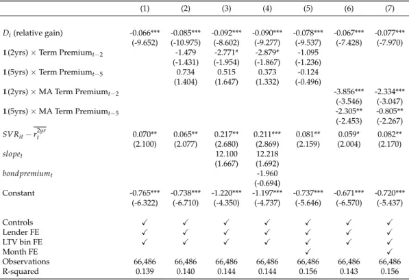
in Figure1.1, which plots the average refinancing probability conditional on the

rel-ative gain in case of inaction. Refinancing is significantly less frequent when gains are positive. This evidence is at odds with models of optimal refinancing (Agarwal,

Driscoll, and Laibson, 2013). Since past rates are uninformative about borrowing

costs going forward, they should not matter for refinancing choices.

The idea that the utility of an outcome is a function of the outcome’s distance from a reference point is a fundamental tenet in prospect theory (Tversky and Kahneman,

1981). Extensive evidence from laboratory experiments and field studies documents

the importance of framing effects on decision making.2 While this paper is the first

to look at the effect of reference points on mortgage refinancing decisions, in finance reference-dependence has been studied in a number of other settings (Baker, Pan,

and Wurgler, 2012; Loughran and Ritter, 2002), including borrowing markets and

housing decisions. Closest to this paper are the results in Dougal et al.,2015, which

shows from the syndicated loan market that firms borrowing rates seem unduly in-fluenced by previous rates, providing evidence that uninformative historical infor-mation may enter negotiations through the effect of reference points. Andersen et

al.,2019and Genesove and Mayer,2001study anchoring and reference dependence

in listing premia in the housing market and find that listed prices increase sharply when households face nominal losses. While previous work establishes the role of reference points or anchors to simplify the complex tasks of valuation and negotia-tion, in my setting there is no bargaining between borrowers and lenders or buyers and sellers, and there is no concern about the endogenous timing of the choice with respect to the nominal loss. Moreover, the large effects of reference points that I es-timate are particularly puzzling given the large amount of money left on the table: between 2013 and 2017, households that do not refinance pay on average an interest rate 2.26 percentage points higher than current market rates.

Reference points and deviations from them arise from the design of the typical mort-gage in the UK. Unlike in the United States, long-term fixed rate mortmort-gages are not available in the UK. In fact, most borrowers are on an initial fixed rate mortgage for a short period of time (typically 2 or 5 years), after which the mortgage reverts to a variable rate for the remainder of the term. Once the fixed period ends, borrowers 2_{For a comprehensive survey of the literature see e.g. Barberis,}_{2013; Beshears et al.,}_2018;

(11)

1.1. Introduction 3

Figure 1.1: Conditional Refinancing Probability

The figure shows average refinancing probability conditional on the relative gain in case of inaction, expressed in percentage of the outstanding loan balance. This is the difference between the rate on the expired initial deal and the reversion rate (SVR) that applies after the reset. In the positive region, bor-rowers that do not refinance experience a decrease in monthly payments if they revert to the SVR. The relative gain is instead negative for borrowers who would experience an increase in monthly payments by reverting on the SVR at the end of the initial fixed period. For this figure, I restrict my sample to mortgages that have a LTV between 60% and 75%, and an outstanding balance between £100,000 and £250,000 at reset. This corresponds to 7,594 observations. The red bars show 95% confidence intervals for the conditional mean.

can refinance to a new initial deal without incurring a prepayment penalty. Paired with the fact that reversion rates tend to be much higher than current market rates, this creates a strong incentive to refinance around the reset date. While reversion rates and current market rates determine the savings foregone by households that fail to refinance, the change in mortgage payments experienced in case of inaction depends on the just expired initial fixed rate. I posit that borrowers evaluate the benefits from refinancing relative to this expired fixed rate, which is a natural can-didate for a reference point in this context. I test this hypothesis using loan-level data where I can follow borrowers’ refinancing behavior after the initial fixed period ends, and which allows me to observe both the matured fixed rate as well as the reversion rate that applies by default. I find that the difference between the matured fixed rate and the reversion rate is a significant predictor of the heterogeneity in re-financing decisions among borrowers, after controlling for differences in potential savings, mortgage characteristics and observable demographics.

The empirical strategy I propose in this paper leverages different institutional fea-tures of the UK mortgage market to identify the causal effect of reference points on refinancing decisions. The main advantage of using UK data is that the design of

(12)

mortgages implies that the status quo level of payments is not preserved in case of in-action. This induces cross-sectional variation in gains and losses with respect to the reference point that is essential to test for reference dependence in how borrowers refinance. A second key feature is that in the UK there is no ex-post price discrimina-tion based on borrower-specific characteristics, including credit scores and income. This rules out obvious endogeneity concerns about past mortgage rates with respect to refinancing opportunities. One would otherwise worry that borrowers who were paying higher rates in the past will naturally face higher rates upon refinancing as well. Crucially, mortgage rates in the UK are quoted by lenders as a discrete

sched-ule at maximum Loan-to-Value (LTV) ratio in steps of 5 to 10% (Best et al.,2018) and

apply to all eligible borrowers at a given point in time. I will therefore argue that

lender×reset time×LTV-buckets fixed-effects absorb all hetereogeneity in rational

refinancing incentives across borrowers, after controlling for mortgage size and re-maining time to maturity. The reason for this is that borrowers who reset at the same time, with the same lender and have a similar LTV face the same reversion rate and the same set of refinancing rates.

Unlike other studies, I can rely on cross-sectional identification because there is a well-specified time window in which refinancing becomes a salient choice and where one can therefore easily compare decision outcomes across people. This would clearly not be possible in the case of pre-payable long-term fixed rate mortgages, where borrowers can refinance at any time. In such cases, researchers have to com-pare actual behavior with a model implied optimal benchmark, which can be hard to compute and has to rely on a number of assumptions. Instead, the cross-sectional approach in this paper is based on a simple argument. Since refinancing is optimal if and only if the saving is larger than the sum of the upfront cost and the option value of refinancing in the future, borroweres with comparable mortgage debt, who face the same rate in case of inaction, the same available market rates and the same fees, should all optimally either refinance or stick with the reversion rate. Showing that there are systematic differences in refinancing behavior predicted by backward-looking information provides evidence of reference dependent decisions. Impor-tantly, this statement holds regardless of whether refinancing is actually optimal or not.

In my analysis, I assume that the rate on the initial fixed period is the relevant ref-erence point for refinancing decisions. Anecdotal evidence suggests that people do take their current fixed rate into consideration when they evaluate the benefits from refinancing. Numerous articles in the popular press warn borrowers about the

pos-sible jump in mortgage payments at the end of the fixed period.3 An article in the

Financial Times,2017even refers directly to the large difference between the

rever-sion rate and the maturing fixed rate as a determinant of refinancing incentives (“So there’s motive for people to remortgage? Precisely.”). However, while the status quo 3_{“Every month hundreds of thousands of borrowers reach the end of their fixed-rate mortgage deal.}

In most cases, that means their mortgage payments are set to rise - in some cases by a lot. But you can take action to avert these higher costs.” (The Telegraph,2019)

(13)

1.1. Introduction 5 seems to predict people choices in many settings, including this one, it is less clear

what should determine reference points in theory. K˝oszegi and Rabin,2006; K˝oszegi

and Rabin,2007argue that expectations determine reference points and that the

sta-tus quo only matters when people expect to preserve it in the future. In the context of this paper, it is hard to tell whether the expired rate matters through the current level of payments or because people extrapolate current borrowing costs into the future. Since the reset of the mortgage rate happens on a pre-determined date and reversion rates are observable over time, the change in mortgage payments is pre-dictable. However, it is still plausible to think that borrowers did not budget for the predictable change in payments and would find themselves forced to cut consump-tion unless they manage to refinance their mortgage. An alternative explanaconsump-tion is that the sudden jump in payments serves as a wake-up call for borrowers, who will check the current level of interest rates if and only if the interest rate increase. Oth-erwise, if interest rates decrease, borrowers will not make the effort of looking at the new available rates and will not realize that savings can be made.

The analysis faces three main identification challenges due to the lack of random assignment of reference points. The variation in past rates that I use to estimate the effect of reference dependence on refinancing decisions comes primarily from differ-ences in borrowers’ choices about the length of the initial fixed interest rate period. While this would not be problematic in general, during the sample period there is a strong positive correlation between past rates and the length of the fixation period because of steadily falling mortgage rates since the financial crisis. The first concern is that unobserved borrower characteristics that simultaneouly explain both a prefer-ence for less duration risk and a lower propensity to respond to financial incentives

might be driving my results (Koijen, Van Hemert, and Van Nieuwerburgh, 2009).

I present a battery of results to show that confounding unobserved heterogeneity in preferences for initial deal duration are unlikely to explain my findings. First, I show that at least in terms of observable characteristics, borrowers that at the same point in time choose different fixation periods are largely similar. Then, I use data from the BOE/NMG Survey of Household Finances to shows that in a period where longer fixation did not imply higher reference rates, borrowers that are expected to have a preference for bearing less duration risk were refinancing more frequently than the average borrower. Lastly, from a placebo regression on a subsample of loans that reset with similar past rates, I demonstrate that initial mortgage dura-tion has no significant effect on refinancing probabilities. The second concern is that borrowers that choose shorter fixation periods are faced with refinancing decisions more frequently. This might both introduce survivorship bias and make borrowers on shorter fixation periods more experienced due to learning through repeated refi-nancing. I address both issues looking at borrowers that are faced with a rate reset for the first time. I show that the effect of reference points on refinancing decisions is still strong in a subsample where survivorship is ruled out and borrowers are ex-pected to be equally experienced. Third, an alternative explanation for my findings is that borrowers that select into longer maturities face a higher probability of being

(14)

denied refinancing. This is a concern given the results in Hertzberg, Liberman, and

Paravisini,2018, which shows from the peer-to-peer lending market in the US that

borrowers with higher unobservable repayment risk tend to self-select into longer maturity contract based on private information. I show that results do not change when I control for the incentive to self-select based on unobservables using the esti-mated difference in term-premia between 2 and 5-years maturities at the time of the origination of the mortgage.

Refinancing decisions play a key role for the effectiveness of monetary policy in stimulating aggregate consumption by reducing the cost of debt servicing. Reflect-ing this policy importance, there has been a surge of papers in recent years that investigate frictions to refinancing. After accounting for the effect of negative

eq-uity (Beraja et al., 2018; Agarwal et al., 2015b), upfront costs and documentation

requirements (DeFusco and Mondragon,2018) in inhibiting refinancing especially

during recessions, a number of papers document that households do not refinance

optimally (Andersen et al., 2015; Agarwal, Rosen, and Yao, 2016; Bajo and Barbi,

2018; Campbell,2006; Johnson, Meier, and Toubia,2019). In particular, Keys, Pope,

and Pope (2016) show that more than 20% of households in the US are paying too

much for their mortgage, incurring a median loss of more than $10,000 in present value terms. Some papers then investigate the determinants and the heterogeneity

of sluggishness in refinancing. Using Italian data, Bajo and Barbi (2018) find that

this “financial apathy” is strongly related to socio-demographic characteristics and

household financial literacy. Andersen et al. (2015) use loan-level data on mortgages

in Denmark to try to quantify the relative importance of two sources of inactivity, namely inattention and inertia. While inertia is supposed to disappear when interest rate incentives are sufficiently large, inattention can prevent people from refinanc-ing even when the incentive to do so is strong. The paper exploits the difference in implied refinancing dynamics to quantify the relative importance of these two chan-nels. While both drivers appear to be important, inattention seems to be the main determinant of low refinancing among households with a low socio-economic

sta-tus. Johnson, Meier, and Toubia (2019) analyze administrative data on pre-approved

offers and argue that time preferences and lack of trust are leading factors explain-ing the low refinancexplain-ing rates observed in their sample. While suspicion towards financial institutions seems to be one of the motives that prevent households from

refinancing, Maturana and Nickerson (2018) show that peer effects can strongly

in-crease refinancing rates. The results in my paper make several contributions to this literature. First, my paper is the first to provide empirical evidence that the fact that missing out on a saving opportunity does not constitute a nominal loss significantly decreases households’ propensity to refinance. Second, my results imply that the responsiveness of a borrower not only depends on individual attributes such as fi-nancial literacy, but is crucially affected by the “framing” of the refinancing gains. Third, a lot of the engagement in the refinancing market in the UK seems to be moti-vated by the desire of avoiding a nominal loss, and this can be easily misinterpreted as a sign of financial sophistication. This could lead to wrong estimates about the

(15)

1.2. Mortgage Design and Reference Points in the UK 7 actual responsiveness of mortgages when interest rates go down in a recession and thus overestimate the stimulating potential of expansionary monetary interventions. This paper fits therefore more broadly in the rapidly growing literature on the role of mortgage markets and security design in the transmission of monetary policy

through the refinancing channel (Abel and Fuster,2018; Auclert,2019; Berger et al.,

2018; Di Maggio, Kermani, and Palmer,2016; Eichenbaum, Rebelo, and Wong,2018;

Fuster and Vickery,2014; Greenwald, 2018; Wong, 2019). I establish an important

complementarity between monetary policy and the decisions of mortgage lenders in the UK about where to set reversion rates, which appear to be crucual in amplify-ing refinancamplify-ing frictions comamplify-ing from behavioral biases. In a similar spirit to Berger

et al., 2018, who argue that the average outstanding rate on fixed-rate mortgages

leads to a path-dependent effectiveness of monetary policy through the incentives to prepay, my results show that in the UK the effectiveness of the refinancing chan-nel of monetary policy depends on the distribution of reference points and, more precisely, of the expected nominal gain in case of inaction. Finally, the evidence pro-vided in this paper about borrowers’ reluctance to taking action also relates to the literature on the effects of default options on economic outcomes (Beshears et al.,

2009; Beshears et al.,2015) which finds, in a number of different settings, a strong

tendency of people against opting out that is hard to reconcile with any plausible value of transaction costs.

The rest of the paper is organized as follows. Section1.2describes the institutional

backround of my analysis. Section1.3introduces the theoretical framework. Section

1.4presents the empirical strategy. Section1.5describes the data and sample I use.

Section1.6presents the main empirical results and Section1.7addresses a number

of identification challenges. Section1.8concludes.

1.2 Mortgage Design and Reference Points in the UK

Unlike in the United States, where the most common product is a 30-years fixed rate mortgage, homeowners in the UK can lock in their mortgage rate only for limited periods of time. The typical mortgage charges an initial fixed rate for a period of 2-5 years, at the end of which the mortgage automatically reverts onto the current Standard Variable Rate (SVR) of the lender. At the end of the initial fixation period, the borrower has the option to refinance to a new initial deal at current market rates without penalty. Borrowers rarely prepay before the end of the introductory deal since most contracts feature large early repayment fees, typically 5 percent of the outstanding loan amount (Best et al., 2018, Cloyne et al., forthcoming). At the end of the fixed rate period, the incentive to refinance is strong for most borrowers. In fact, SVRs charged by lenders are usually susbtantially higher than new fixed or variable market rates quoted at the same point in time. Reversion rates are therefore expensive relative to market rates and households who do not refinance might be missing out on considerable savings. Moreover, even though the SVR is a variable rate and is

(16)

therefore expected to go up when interest rates increase, there is no guarantee that it will fall if interest rates decrease. This is because each mortgage lender sets its own SVR and can revise it at any time, with no obligation to follow the BOE’s base rate or any wholesale rate.

This mortgage design implies that, on pre-determined dates, borrowers come off the fixed rate that they have been paying for the previous 2 to 5 years and are faced with the choice whether to refinance to a new fixed rate or to stay on the SVR of their lender. While lenders usually set their SVR above market rates, whether the SVR is above or below a given borrower’s matured fixed rate at the end of her initial period also depends on the path of interest rates between the origination and the expira-tion of the fixed deal. This means that by reverting onto the SVR some borrowers might see their monthly mortgage payments go down. For these borrowers, the ex-pensive SVR is therefore cheap relatively to their own past rate. On the contrary, for borrowers who expect their mortgage payments to go up at the end of the initial period, the SVR is expensive both relative to market rates and relative to the expired fixed rate. In the data, the distribution of matured fixed rates around the SVR varies over time and, at any given point in time, we can observe substantial cross-sectional heterogeneity.

Figure1.2plots average quoted 2-years and 5-years fixed rates (solid lines), as well

as the average SVR applied by mortgage lenders (dashed line) from 2000 to 2017. I focus on these two maturities (fixation periods) because they are by large the most common in the UK. The cut of the base rate by the BOE at the end of 2008 led to a visible structural break in the relationship between mortgage market rates and reversion rates. Historically, SVRs have been moving at a almost constant spread over market rates, but lenders stopped adjusting their SVRs downward as soon as the policy rate hit the zero-lower bound. Under considerable public and political

pressure to pass-through the interest rate cut (The Guardian,2008), lenders initially

decided to lower SVRs. They did not however follow through once the BOE cut the base rate further by 150 basis points. Despite falling interest rates, average SVRs

remained solid around 4%, and even increased in the following years.4 As a

conse-quence, reversion rates and rates on newly originated mortgages started to diverge and by the second half of 2013 the implied spread was higher than it had been before the crisis.

In the left panel in Figure 1.3, I plot the difference in annual payments between

staying on the SVR and refinancing to a new 2-years fixed rate deal for a typical mortgage with a £100,000 remaining balance, 20 years left to pay down the princi-pal and a LTV of maximum 75%. For around two years after the crisis, reversion rates were at the same level of market rates, or even cheaper. As financial markets recovered and risk premia went down, foregone savings for households that failed 4_{A similar pattern to the one observed in the UK is documented in Goggin et al. (2012) for the Irish}

market and the authors attribute the unwillingness of banks to pass-through interest rate cuts onto their reversion rates to increased market funding costs.

(17)

1.2. Mortgage Design and Reference Points in the UK 9

Figure 1.2: Mortgage Rates

The figure shows monthly time series of average quoted interest rates for different mortgage products and of the Bank of England base rate. The dark solid lines is the interest rate on a 2-year fixed initial period for a maximum loan-to-value of 75%. The lighter solid line is the corresponding rate for a 5 years initial duration. The dashed line is the average standard variable rate (SVR) applied by financial institutions. All mortgage rate series are taken from the Bank of England Interactive Database.

2001 2003 2005 2007 2009 2011 2013 2015 2017 0 1 2 3 4 5 6 7 8 SVR BOE base rate 2-yrs fixed 5-yrs fixed

to refinance began to grow larger. Between 2013 and 2016, which is the period cov-ered by my data, the average SVR was 4.44% against an average 2-years fixed rate of 2.18%, corresponding to an average annual difference in mortgage payments of £1,424.

The right panel of Figure1.3 shows the change in mortgage payments implied by

inaction relative to the expired deal. Right after the crisis, not only the incentive to refinance plotted in the left panel was small or negative, but borrowers reverting to the SVR would see their mortgage payments decrease substantially. From 2011, two things happen. First, the expected change in mortgage payments in case of in-action began to increase, and more and more borrowers reverting to the SVR would experience a jump in mortgage costs. Second, we observe a large difference in the experienced change in payments at reset for 2-years versus 5-years mortgages. On average, in the period 2013-2016, borrowers coming off a 2-years fixed deal saw their payments go up by £931 per year. At the same time, the rate reset meant a decrease in annual payments by £565 if the borrower had instead locked in the fixed rate five years before for five years. Because of steadily falling interest rates and high term premia after the crisis, borrowers on a 5-years contract were paying on average 2.3% points more in interest charges than borrowers on a 2-years contract resetting at the same time.

Standard models of optimal refinancing would predict no difference in refinancing behavior across borrowers that experience an increase versus a decrese in mortgage

(18)

Figure 1.3: Incentives to Refinance

This figure shows the evolution of the incentives to refinance over time, decomposed into the potential savings from refinancing (left) and the cost of staying on the SVR (right). Calculations consider a borrower with a repayment mortgage, £100,000 remaining balance and 20 years left until maturity. Specifically, the line in the left panel shows the change in annual payments when switching from the SVR to a new 2-years fixed rate initial deal, computed as P(SVRt) −P(r2yrt ). The right panel

shows the change in annual payments when moving onto the SVR for mortgages coming off a 2-years (darker line) or a 5-years (lighter line) fixed deal, i.e it plots P(SVRt) −P(r2yr_t−2)and P(SVRt) −P(r5yr_t−5),

respectively. At each point average quoted rates for mortgages with a maximum LTV of 75% are considered. 2005 2007 2009 2011 2013 2015 2017 2000 1500 1000 500 0 500 1000 1500 2000

2500 Gross Savings from Refinancing

2005 2007 2009 2011 2013 2015 2017 2000 1500 1000 500 0 500 1000 1500 2000 2500 Cost of Inaction 2 years 5 years

payments relative to the expired fixed rate. However, finding that this dimension matters in borrowers decisions, has implications for the effectiveness of monetary policy in reducing mortgage payments and stimulating household consumption. The pass-through of monetary policy is stronger on rates on newly originated

mort-gages due to competition among lenders (Scharfstein and Sunderam, 2016), thus

the central bank has traction on refinancing incentives through the level of foregone savings. On the contrary, the cost of inaction, defined as the difference between current SVRs and past market rates, responds less and with a delay to monetary policy interventions. First, because it depends on the path of interest rates in the past and, second, because the pass-through of interest rates is limited by lenders’ market power on their current clients.

1.3 The Theoretical Framework

Following the literature on optimal mortgage refinancing (e.g. Agarwal, Driscoll,

and Laibson, 2013; Andersen et al., 2015), we can write the incentive to refinance

as

I =r0−r1−x∗ (1.1)

where r0is the interest rate in case of inaction, r1is the interest rate on the new

(19)

1.3. The Theoretical Framework 11 option value of refinancing in the future. All variables are time varying, but I drop the time subscript for convenience. A borrower that maximizes the utility in the out-come state will refinance if and only if the incentive to do so is positive, i.e. when

I > 0. Agarwal, Driscoll, and Laibson,2013are the first to derive a closed form

so-lution to the household’s refinancing problem under a plausible set of assumptions, which other authors have used as rational benchmark against which to define

refi-nancing mistakes (Keys, Pope, and Pope,2016). Andersen et al.,2015extend this

ra-tional model to incorporate inertia to generate heterogeneous responses to identical financial incentives. In particular, they allow the psychological cost that borrowers’ associate with refinancing to vary across-borrowers, resulting in borrower-specific

threshold levels x∗. The authors investigate how the estimated inertia covaries with

borrower and mortgage characteristics and find it increasing in households’ socio-economic status.

In this paper, I posit that borrowers have reference dependent preferences and eval-uate the benefits from refinancing relative to individual reference points. Under this assumption, heterogeneous reactions to the same financial incentive may result from differences in reference points, even after controlling for borrower characteristics to proxy for financial literacy. This hypothesis is consistent with a model that assumes

that household’s utility function u(C|R)depends on the consumption level C and a

reference level of consumption R. Reference dependence is a fundamental principle in prospect theory and it is captured by the value function defined on the difference

C−R in Kahneman and Tversky,1979. Building on this theoretical framework, I

specify a borrower’s utility function in terms of interest rates as

u(r|rR) =µ(rR−r−κ(rR, r)) (1.2)

where r is a mortgage rate, rR is the reference mortgage rate and κ(rR_{, r}₎_{is the}

po-tential cost involved with moving from the reference state to the new state, which

reduces consumption in the outcome state. µ(·)is a gain-loss function that satisfies

the following properties:

A0. µ(x)is continuous for all x, twice differentiable and µ(0) =0 A1. µ(x)is strictly increasing.

A2. µ00(x) ≤0

Notice that I am not assuming a kink at the reference point, as in the well-known S-shaped value function in prospect theory. Because of the diminishing marginal utility resulting from concavity, the disutility from a loss is still larger in absolute value than an equally sized gain. What this specification does not assume, is di-minishing sensitivity to losses, i.e. that the marginal disutility of a further loss in consumption decreases as the loss grows larger.

(20)

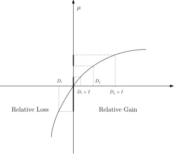
Figure 1.4:Value Function Dj+I Dj Di+I Di µ Relative Gain Relative Loss

Assuming a strictly positive psychological cost of taking action ζ, a borrower i with reference rate rR

i will refinance if and only if the change in utility is large enough to

compensate for the hassle of refinancing, i.e.

µ(r_iR−r1−x∗) −µ(rR_i −r0) =µ(Di+I) −µ(Di) >ζ (1.3)

where

Di ≡rRi −r0 (1.4)

is the distance of the reversion rate from the reference rate, expressed as a gain. I introduce the subscript i to stress that the reference point can vary across households for given r0 and r1. In the first term of the equation, κ(rR, r1) = x∗ captures the

financial cost of refinancing that enters (1.1). By definition, there is no cost involved

in reverting to the reversion rate r0, so κ(rR, r0) =0 in the second term.

Equation (1.3) implies that a positive rational incentive I > 0 is a necessary

condi-tion, but not a sufficient for ζ > 0. Moreover, given concavity of µ, the propensity

to refinance is negatively related to Di. In other words, the higher the relative gain

(or the smaller the relative loss) of reverting to r0_{, the smaller the increase in}

util-ity from refinancing to a lower r1. The intuition is visualized in Figure1.4, where I

draw an hypothetical value function to sketch the refinancing problem for two

bor-rowers i and j with two different reference rates. Diand Djon the x-axis indicate the

change in interest rates in case of inaction and determine the experienced change

in monthly payments. Di is negative meaning that r_iR < r0. In this case, inaction

implies a loss in consumption and therefore a lower utility relative to the reference

(21)

1.4. Empirical Strategy 13 borrower j experiences a drop in monthly payments once the mortgage rate resets. Given the same incentive I, refinancing implies an increase in utility indicated in bold on the y-axis for the two borrowers. However, notice that for borrower i, the perceived benefit from refinancing is much larger. This is because refinancing in-cludes an additional increase in utility coming from avoiding a out-of-pocket loss relative to the reference point. The utility increase from gaining I, is instead much smaller for borrower j since, from her point of view, action only implies realizing an additional saving. Because of the assumption of decreasing sensitivity to gains, the same level of I might therefore not be enough to motivate borrowers who do not see the inaction state as a loss state into refinancing to a lower rate. The following testable hypothesis summarizes this idea:

Hypothesis (Reference Dependence). Given an action state and an inaction state, the incidence of refinancing in the cross-section of borrowers is negatively related to the difference D between the rate on the expired deal (reference rate) and the rate in the inaction state.

1.4 Empirical Strategy

To test the hypothesis of reference dependence in refinancing decisions, I exploit the variation in reference points across borrowers whose fixed rate resets at a pre-determined date. Formally, I run the following specification

Re f inancei =αt,l,LTV+βDi+γ0Wi+εi (1.5)

where Re f inancei is an indicator variable denoting whether loan i refinances after

the reset and Di is the distance between the reference rate and the reversion rate

defined in equation (1.4). αt,l,LTV is a time*lender*LTV fixed effect and Wi is a vector of loan-level observables.

A key challenge to identify the effect of reference points on refinancing behavior is to control for differences in refinancing incentives. I leverage on three specific institutional features of the UK mortgage market to overcome this issue. In particu-lar, I take advantage of the fact that (i) borrowers at the same lender face the same reversion rates at any point in time, (ii) mortgage pricing does not depend on bor-rowers’ characteristics and (iii) borrowers can refinance to a different product with their current lender at a minimal hassle. As I explain in detail in the next paragraph, it follows that including granular three-way fixed effects for the time of the reset, the lender and the LTV of the mortgage at reset absorbs observable and unobservable

heterogeneity in monetary incentives as defined in equation (1.1).

Rational incentives to refinance are positively correlated with the rate r0

i that the

borrower is charged if she decides not to refinance. In the present context, this is the SVR to which the borrower automatically reverts at the end of the deal. This rate is constant for borrowers who have a loan with the same lender and whose initial

(22)

rate resets at the same time, and it is observable. The second term r1_i in equation

(1.1) is determined by the current level of interest rates and more precisely by the

set of interest rates that are available to a given borrower at a given time. Mortgage products in the UK are very standardized and for any given product lenders offer the same interest rate to all borrowers that meet their lending standards. In particu-lar, interest rates do not depend on individual borrowers’ creditworthiness or other characteristics. Differently from the United States, where mortgage rates are quoted to borrowers individually and are a function of their credit score, default risk in the

UK is priced based on the LTV ratio. Best et al.,2018 confirm in the data that

af-ter controlling for bank, time, inaf-terest rate (fixed or tracker), length of the initial deal and type of repayment (interest only or principal amortization), what determines the interest rates is the LTV ratio. In particular, the average mortgage interest rate is a step function of the LTV ratio, with sharp jumps (notches) at LTVs of 60%, 70%, 75%, 80% and 85%, and flat in between. Moreover, unlike in the US where many lenders

offer different interest rates across states5, in the UK mortgage rates do not vary

across zipcodes or regions. Most products are available throughout the UK, even though some providers have limited lending areas. It is possible that some products

are only available online, in branch or via an intermediary (MoneyFacts.com6_{). It}

follows that the same set of interest rates is in principle available to all borrowers

that reset at a given time and whose LTV ratio falls within a given range, so that r1_i

is constant within this cluster. The last term x∗_i is both increasing in the up front cost of refinancing and in the option value of waiting and refinancing at a future date. Refinancing is costly, both in terms of money and time. There is however a sub-stantial difference between refinancing with the current lender (product transfer) or with a new lender. When transferring to a new mortgage with the current lender, no fees are usually charged and the procedure is commonly a matter of days and can be done entirely online. This is because for existing clients lenders usually do not require a new valuation of the property nor updated affordability checks, provided that the terms of the contract are unchanged. If the borrower wishes to modify the length of their term, increase the borrowed amount or change the repayment type of the loan, the lender will request a new assessment of both the financial situation and the value of the house. Thus, the cost of refinancing to the same product im-plies a different cost for new and existing clients of the mortgage provider. In turn, this affects refinancing incentives across borrowers, even though in principle they face the same set of available market rates. Lender fixed effects absorb this hetero-geneity across borrowers at different lenders in accessing the same rate. Including lenders fixed effects also controls for differences in average refinancing probability, which may result from some lenders having more stringent requirements, higher fees, lenghtier procedures and different clienteles. Finally, the option value of wait-ing and to refinance in the future depends on the stochastic process of interest rates. I assume that, after including time fixed effects, borrowers expectations about future

5

https://www.consumerfinance.gov/about-us/blog/7-factors-determine-your-mortgage-interest-rate/

(23)

1.5. Data and Sample 15 interest rates are unrelated to reference points.

The vector Wi includes control variables that are expected to influence borrowers

incentive to refinance and that are not absorbed by the fixed effects. In particular, I control for the remaining balance on the mortgage given that, since interest savings from refinancing scale proportionately with mortgage size but refinancing cost is

fixed, x∗ is decreasing in mortgage size. Moreover, since the remaining time until

maturity of the loan affects the option value of waiting, I include it as a control in the regression. Given the extensive set of fixed effects required to make robust inference, I first estimate a linear probability model.

At each point in time, the distribution of reference points across borrowers depends on the path of interest rates up to that point. Because of steadily declining interest

rates, the right panel in Figure1.3shows that in the sample period Di is positively

related to the length of the fixation period of the maturing deal. The key

identi-fying assumption for equation (1.5) to estimate the causal effect of Di on

refinanc-ing decisions is that preferences for duration risk are uncorrelated with borrowers’ propensity to show inertia or inattention or with other characteristics that may ex-plain sluggishness in refinancing behavior. Borrowers’ age and income have been shown in the literature to correlate with borrowers’ responsiveness to refinancing

incentives. Using data from the American Housing Survey (AHS), Campbell,2006

shows that most active refinancers are younger, better educated, white households

with higher-priced houses. Andersen et al.,2015find similar results studying the

Danish mortgage market. I can observe borrowers’ age and income in the data, so I include them as controls in the regression. While age and income may affect the probability of refinance, they should not change the coefficient of interest since in

the UK interest rates are not related to borrower characteristics. Still, since Di is not

exogenously assigned, I need to assume that there are no unobserved characteristics

that are correlated with both Diand refinancing decisions. In Section1.7.1, I provide

a set of additional results to rule out that my findings are driven by unobserved bor-rower characteristics simultanously driving duration and refinancing choices.

1.5 Data and Sample

1.5.1 Data Sources

For the main analysis I use a novel loan-level panel dataset on more than 2 mil-lion securitized residential prime mortgages in the UK provided by the European

DataWarehouse (ED).7 Data start in January 2013 and my sample ends in August

7_{ED collects loan-level information on the pool of loans backing RMBS that financial institutions}

pledge as collateral in Eurosystem refinancing operations. Following the eligibility requirements set by the ECB, since January 2013 participants to the Eurosystem have to submit updates on the underlying loans at least on a quarterly basis. As part of a measure to preserve collateral availability and market functioning, on September 6, 2012, the ECB extended eligibility to be used as collateral in Eurosystem credit operations to marketable debt instruments denominated in GBP (or US dollar or Japanese yen).

(24)

2017. In terms of coverage, the loans in the dataset correspond to roughly 10% of the

total amount outstanding of mortgages in the UK over the period.8The dataset

con-tains detailed information on the loans, including the name of the loan originator, the loan size, the origination date, the interest rate charged, whether the mortgage payments include amortization of the principal, the valuation of the property, the mortgage term over which the loan will be fully repaid, as well as the geographical location of the property at county level (NUTS3). The data also provides informa-tion on the purpose of the loan (purchase, re-mortgage, renovainforma-tion, equity release, etc.), if it is a first or second mortgage and whether the mortgage is buy-to-let or owner-occupied. The data includes a number of borrower characteristics as of loan inception, namely age, income, income verification, employment status, credit score and whether the borrower is a first-time buyer.

The frequency of the data is either monthly or quarterly.9 At each submission, I

observe updated information on the payment history (current, in arrears, defaulted or prepaid) as well as the type of the mortgage and the interest rate charged. In particular, I know if the loan is currently on an initial (fixed or floating) rate, on the lender’s SVR or on another rate (e.g. lifetime BoE base rate tracker, capped or discount). For introductory deals I observe the date when the deal ends and the loan reverts onto the follow-on rate unless the borrower refinances. In case the reset date is missing in the data, I recover it from the changes in the interest rate and the interest rate type across submissions. The dataset contains a variable that indicates the type of follow-on rate, whether it is the lender’s SVR or another tracker rate.

Once the introductory period ends, I see from the following submissions if and when the borrower decides to refinance. If the borrower does not refinance, the loan ap-pears on the lender’s SVR. If the borrower decides to switch to a new product with the current lender, I observe the selected mortgage type and the new interest rate. Usually, borrowers that refinance after being on a fixed rate opt for a new initial fixed rate deal. If, instead, the borrower decides to remortgage with a different lender, re-financing appears in the data as a prepayment, after which the loan stops being reported.

The dataset contains updated information on loans’ current balance and current loan-to-value ratio. For property values reported in the data and used to compute the current loan-to-value, I observe two reporting practices that vary across, but are consistent within, lenders. Most lenders update the value of the property at

each submission according to an internal indexing methodology.10 _{Other lenders,}

Disclosure of loan-level information is also one of the eligibility requirements for credit operations with the Bank of England since November 2012. Since the Bank of England has access to the ED platform, many UK issuers use it to fulfill the disclosure requirements. Some issuers prefer alternative ways. Over the period 2013-2019, coverage of the UK RMBS market by the ED dataset varies between 30 and 60%.

8_{Data on total balances outstanding are from the Bank of England and the FCA.}

9_{The frequency at which data are submitteed to ED depends on the RMBS coupon schedule.} 10_{The data contain information on the valuation type used at each submission. Most of the properties}

are valued according to a full internal and external inspection at origination of the loan. On subsequent dates, if the property value is updated the valuation method is typically indicated as Indexed.

(25)

1.5. Data and Sample 17 instead, report an updated property value only upon refinancing of the loan and usually only if the balance of the loan increases. Both behaviors are consistent with the fact that lenders usually do not require a new full valuation of the property in case of internal refinancing, except in case of modification of the loan terms. It is possibile that also lenders that report constant property values may use an indexing methodology before granding a product transfer to an existing client. For my anal-ysis, I assume that the reported loan-to-value is the relevant one to determing the available set of refinancing rates. For robustness, I will include county fixed effects in some specifications in order to control for heterogeneity in house price growth across counties.

1.5.2 Sample Selection and Summary Statistics

Table 1.1 shows a snapshot of the cross-section of mortgage types as they are

ob-served at the beginning of the sample in 2013. I see that a large fraction of borrow-ers (61%) are paying the SVR, which is surprising given that market rates in 2013 were already significantly cheaper. Since for borrowers with a small balance or few years left to maturity the potential savings might not justify the cost and hassle of refinancing, in the second row I restrict the sample to borrowers with a remaining balance higher than £100,000 and more than ten years to term. Since premia charged to highly leveraged borrowers increased substantially after the crisis, I also exclude mortgages with a LTV ratio higher than 75% to compute these figures. The fraction of mortgages on the SVR drops substantially to 43%, but it is still very large consid-ering that borrowers in this subsample are foregoing substantial amount by failing to refinance to a new initial deal. To study reference dependence in refinancing de-cisions, I focus on mortgages on an initial fixed rate period.

In the early 2000s two major lenders guaranteed to their clients that their SVR would never rise more than 2% above the BoE base rate. Since the cut of the base rate in 2009, these reversion rates have been below most available market rates, which led the lenders in question to introduce a second, more expensive SVR for the newly originated mortgages. Since most mortgages in the dataset were originated before 2010, 30% of the loans in ED are on a low reversion rate as of their first submission.

These loans are not considered in Table1.1 since they imply low or negative

incen-tive to refinance. Mortgages that are first observed on an initial fixed rate, but which are meant to revert to a low reversion rate, are also excluded from the analysis. Like in most studies on the failure to refinance, one concern is that some borrowers might want to switch to a lower rate but cannot because ineligible to do so. The distribution of housing equity and unemployment might contribute to explain some of the observed sluggishness in refinancing behavior, since borrowers are likely to be denied refinancing if the account is in arrears, they have little or no equity, or there

have been material changes in their circumstances (Agarwal et al.,2015b; Beraja et

(26)

Table 1.1: Distribution of Interest Rate Types (2013)

This table shows the fraction (in %) of mortgages by interest rate type at the beginning of the ED sample (2013). In the first row, reported figures are computed over all mortgages in the sample except for those on a lifetime tracker rate, which mostly indicates mortgages on a reversion rate that was guaranteed not to rise more than a small margin (usually 2%) above the BOE base rate. The second row only considers borrowers who have a remaining balance higher than £100,000, more than ten years left until maturity and a LTV ratio at reset not larger than 75%. The column SVR indicates the fraction of borrowers that are on their lender’s Standard Variable Rate as of the first time they are observed in the data. Initial Fixed (Floating) indicates mortgages that are on an initial fixed (variable) rate and that will automatically revert to the SVR at the end of the deal. Other includes capped and discount mortgages.

SVR Initial Fixed Initial Floating Other N

All borrowers* 61.05 26.12 5.71 7.11 1’478’446

Borrowers with

a strong incentive 43.18 42.13 8.07 6.62 227’424

qualify for a new mortgage due to bad performance or negative equity, I restrict my analysis to borrowers that were never reported late on their payments and who reset with a loan-to-value ratio below 90%. Still, these criteria cannot identify borrowers who are excluded from refinancing despite having positive equity and never missed a payment because they no longer meet lenders’ eleigibility requirements, which have become stricter after the crisis and, in particular, since the introduction of the Mortgage Market Review in April 2014 in the UK. The cases of borrowers trapped in expensive reversion rates have attracted considerable attention in the popular press. According to those accounts, these so-called mortgage prisoners appear to be mostly self-employed or elderly people, who took out interest-only or self-certified mortgages. Moreover, as also reported in the FCA 2019 Mortgage Market Study, most of these mortgages are with unauthorized or inactive lenders, who do not offer any new deals. I do not expect this to be a major issue for my analysis for two reasons. First, there are no mortgages originated by currently inactive lenders in the data and servicer and originator are the same for the vast majority of loans. Second, in the regressions I control for income certification, repayment method, dummy for first-time buyers and age of the borrower, which I require to be non-missing. I also drop loans for which there is no information about the location of the property to rule out that my results are capturing heterogeneity in regional house price growth.

In Section1.6.3, I show that my results are robust to these restrictions.

The final sample constains 85,830 reset events distributed fairly homogeneously

be-tween January 2013 and August 2017. Table1.2presents summary statistics for the

mortgages in the sample. The first four columns show number of observations, mean, standard deviation and median for loans that reset to a SVR that is lower than the rate on their past fixed deal. The next four columns present the same sum-mary statistics for borrowers that instead reset to a SVR that is higher than their

(27)

1.5. Data and Sample 19

Table 1.2: Summary Statistics for Mortgages that Experience a Rate Reset

This table shows summary statistics for the mortgages in the analysis sample, which includes only mortgages that see their initial fixed rate reset at some pre-determined date during the sample period. I report number of observations, mean, standard deviation and median of the control variables sepa-rately for mortgages that experience an automatic drop in monthly payments at reset (GAIN) and those who see their payments increase when falling on the reversion rate (LOSS). All variables in Panel A and B are measured at the end of the introductory deal, except for gross income and credit score which are as of the inception of the loan. Loan-to-income is current balance divided by income at inception. Income verification indicates whether the income of the borrower has been verified by the lender when the loan was granted. Reported credit scores in the ED data follow different scales depending on the score provider: Callcredit, Experian or Equifax. To allow comparability, I standardize the score by the maximum value in each score system. For lenders that assign credit scores according to internal systems, I standardize using the maximum assigned value in sample. Panel C reports original loan amount, LTV ratio and term of the loan (in years) as of the origination of the mortgage.

Reset implies GAIN (Di> 0) Reset implies LOSS (Di< 0)

N Mean SD Med N Mean SD Med

Panel A: Loan Characteristics at Reset of the Current Initial Fixed Deal

Interest Rate (%) 30336 5.32 0.83 5.19 55494 3.15 0.58 3.24

Loan Value (1000) 30336 93.62 66.52 81.18 55494 105.24 92.27 81.86

Loan-to-Value (%) 30336 59.32 25.67 67.47 55494 43.84 19.64 44.61

Years to Maturity 30336 17.49 7.85 17.92 55494 13.92 6.62 13.67

Interest Only 30336 0.10 55494 0.22

Panel B: Borrower Characteristics

First-Time-Buyer 30336 0.41 55494 0.19

Gross Income (1000) 30336 38.78 23.50 33.32 55494 46.64 31.59 38.00

Age at Reset (Years) 30336 43.21 10.88 42.00 55494 47.46 9.62 47.00

Loan-to-Income 30336 2.51 1.17 2.48 55494 2.34 1.28 2.21

Income Verification 30336 0.62 55494 0.52

Credit Score 15475 0.75 0.12 0.75 23371 0.78 0.14 0.77

Panel C: Loan Characteristics at Origination

Original Loan Value 30336 106.81 68.39 93.00 55494 126.61 95.83 102.00

Original Loan-to-Value 30331 70.24 23.38 78.40 55481 59.99 21.45 63.60

Original Loan Term (Years) 30336 23.67 6.38 25.00 55494 20.99 6.04 22.00

mortgage payments are lower on the SVR than on the introductory rate. Figure1.9

in the Appendix shows the time series of SVRs by lender.

1.5.3 Distance from the Reference Point

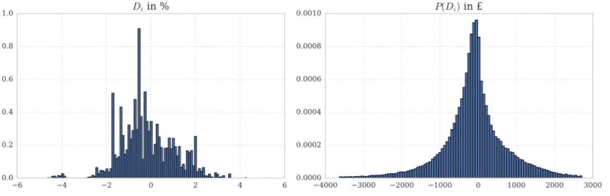
The main explanatory variable of interest is the distance Di between the reversion

rate and the reference rate, defined in equation (1.4). The left panel of Figure 1.5

plots the distribution of this measure in the data. Recall that Di is the difference in

percentage points between the interest rate charged on the introductory deal and the SVR charged in case of inaction. A negative value thus means that reverting to the SVR implies an increase in mortgage payments relative to what the borrower has

(28)

Figure 1.5: Variation in Di

The left panel plots the distribution of Didefined in equation (1.4) as the percentage point difference

between the rate paid on the introductory period and the reversion rate (SVR). The right panel shows the distribution of the change in annual mortgage payments implied by Di(in £).

6 4 2 0 2 4 6 0.0 0.2 0.4 0.6 0.8 1.0 Di in % 4000 3000 2000 1000 0 1000 2000 3000 0.0000 0.0002 0.0004 0.0006 0.0008 0.0010 P(Di) in £

been paying until that moment. In other words, staying on the SVR implies a loss in disposable income from the perspective of the reference point. In my sample, about 40% of resets happen when this distance is negative. The average distance is 9.5 basis points. Since interest rates have been going down over the period under con-sideration, the fraction of borrowers with a negative distance decreases over time, dropping from 53% in 2013 to 32% in 2017. In the right panel, I plot the change in annual disposable income in the inaction state relative to the reference state in the right panel for the borrowers in the sample, which are roughly normally distributed between minus and plus £2,000.

1.6 Results

1.6.1 Graphical Evidence: Losses versus Gains

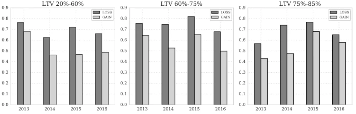
In this section, I provide preliminary evidence that reference points matter for bor-rowers’ refinancing decisions. To do so, I group households based on whether the

SVR is higher (LOSS) or lower (GAIN) than the rate on the fixed deal. Figure1.6plots

the fraction of households that have refinanced their mortgage within six months from the end of the introductory fixed deal, by year of the reset. The left panel considers mortgages with a LTV at reset between 20% and 60%, the center panel mortgages with a LTV between 60% and 75% and the right panel mortgages with a LTV between 75% and 85%. The average refinancing rate across observations

is 62.5%.11 The reference dependence hypothesis posits that we should observe a

11_{Using a comprehensive dataset on the universe of UK mortgages, the Financial Conduct Authority}

(FCA) finds that in the period 2015-2016 more than 75% of the mortgages have been refinanced within six months from the reset. For the same period, the refinancing fraction in my sample is lower, 65.8%. The FCA 2019 Mortgage Market Study can be found at https://www.fca.org.uk/publication/market-studies/ms16-2-3-final-report.pdf.