HAL Id: hal-01386172
https://hal.archives-ouvertes.fr/hal-01386172
Submitted on 23 Oct 2016
HAL is a multi-disciplinary open access archive for the deposit and dissemination of sci-entific research documents, whether they are pub-lished or not. The documents may come from teaching and research institutions in France or abroad, or from public or private research centers.
L’archive ouverte pluridisciplinaire HAL, est destinée au dépôt et à la diffusion de documents scientifiques de niveau recherche, publiés ou non, émanant des établissements d’enseignement et de recherche français ou étrangers, des laboratoires publics ou privés.
SLMRACE: A noise-free new RACE implementation
with reduced computational time
Juliet Chauvin, Edoardo Provenzi
To cite this version:
Juliet Chauvin, Edoardo Provenzi. SLMRACE: A noise-free new RACE implementation with reduced computational time. Journal of Electronic Imaging, SPIE and IS&T, 2017, �10.1117/1.JEI.26.3.031202�. �hal-01386172�
SLMRACE: A noise-free new RACE implementation with reduced
computational time
Juliet Chauvina, Edoardo Provenzia
aUniversit´e Paris Descartes, MAP5, 45 rue de Saints-P`eres, Paris, France, 75006
Abstract. In this paper we present a faster and noise-free implementation of the RACE algorithm. RACE has mixed characteristics between the famous Retinex model of Land and McCann and the ACE color-correction algorithm. The original random spray-based RACE implementation suffers from two main problems: its computational time and the presence of noise. Here we will show that it is possible to adapt a technique recently proposed by Bani´c et al. to the RACE framework in order to drastically decrease the computational time and to avoid noise generation. The new implementation will be called SRACE, for smart-RACE.
Keywords: Color image enhancement, Retinex, RACE, SLRMSR, GIF, SRSR. *Corresponding author: Edoardo Provenzi, [email protected]
1 Introduction
The Retinex theory of color vision proposed by Land and McCann1aimed at providing a
compu-tational model to understand some essential features of color vision such as locality or robustness
with respect to illuminant changes. The Retinex theory has then been used for many other
pur-poses, one of them is perceptual-based color correction: given an input picture taken under any
illumination condition, one would like to transform it in order to induce a color sensation closer to
what a human observer would experience in the scene depicted by the image. This is the Retinex
use that will be considered in this paper.
The original version of Retinex used piecewise linear path to explore the image content around
a point of an image. Several works have been dedicated to the analysis of path geometry which
gives the best performances, see e.g.2–6 The mathematical analysis performed in7allowed pointing
out intrinsic problems related with the use of paths and this led to their replacement with 2-D
sampling structures, called random sprays. This formulation of Retinex is known as RSR for
The spray technique has also been employed to reduce the computational time of another
perceptually-based color correction algorithm called ACE for ‘Automatic Color Equalization’.9
The possibility to use sprays as sampling structure for both ACE and RSR allowed to mix the two
algorithms into a single one with in-between features. The hybrid model is called RACE.10
Even if the spray-based technique is a noticeable improvement with respect to the path-based
one, it is still affected by a high computational time and generation of noise, which affects, in
particular, images characterized by large homogeneous areas.
To overcome these problems, some suitable methodologies has been proposed11,12and applied
to RSR-based algorithms. In this paper we will show that these techniques can be also be adopted
to provide a noise-free and faster implementation of RACE.
Tests and comparisons will show the efficiency of the new implementation with respect to the
original one.
Before starting with the technical content of the paper, let us fix the notation. We will denote
with Ω ⊂ Z2the spatial domain of a digital image of size |Ω| and with x ≡ (x
1, x2) and y ≡ (y1, y2) the coordinates of two arbitrary pixels in Ω. We will always consider a normalized dynamic range
in [0, 1], so that a RGB image function will be denoted with ~I : Ω −→ [0, 1] × [0, 1] × [0, 1],
x 7→ (IR(x), IG(x), IB(x)), where each scalar component Ic(x) defines the intensity level of the
pixel x ∈ Ω in the red, green and blue channel, respectively.
We stress that we will perform every computation on the scalar components of the image, thus
treating each chromatic component separately as in the original Retinex paper.1 Therefore, we
will avoid the subscript c and write simply I(x) to denote the intensity of the pixel x in a given
2 RSR, ACE and RACE
In this section we will describe the algorithms RSR, ACE and their fusion RACE. Let us start with
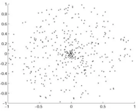
RSR. Fixed a pixel x, N different sprays Sk, k = 1, . . . , N , as the one depicted in Fig. 1, are
centered in x. For simplicity we will consider all the sprays to have the same number of pixels n.
The generic pixel in the spray Sk, different from the center, will be denotes with y and the notation
Hkwill be used to indicate the pixel with highest intensity belonging to the spray Sk (notice that
Hkcan coincide with the center pixel x).
Fig 1 A random spray used in RSR.
The re-computation of pixel intensity performed by RSR is the following:
I(x) 7−→ LRSR(x) = I(x)1 N N X k=1 1 I(Hk) , (1)
for all pixel x ∈ Ω, and for the three chromatic channels separately. Due to the quotient over
the maximal intensity of each spray, RSR belongs to the category of white-patch color correction
algorithms.
To describe ACE, we have to previously define the slope function sα : [−1, 1] → [−1, 1] as follows: sα(t) = −1 if − 1 ≤ t ≤ −1α αt if −1α < t < α1 +1 if α1 ≤ t ≤ 1,
where α > 1 is a slope parameter freely selected by a user. We must also consider a suitably
normalized weight function w, i.e. P x∈Ω
w(x, y) = 1, decreasing with the Euclidean distance kx−yk
and such that w(x, x) = 0.
We can now define the first stage of ACE as the following intensity re-computation:
I(x) 7−→ R(x) = X y∈Ω
w(x, y)sα(I(x) − I(y)), (2)
thanks to the slope function, small intensity differences are amplified and large ones are saturated.
The second, and final, step of the ACE computation is the following global re-mapping:
LACE(x) = 1 2 +
R(x)
2M (3)
where M = max
x∈Ω{R(x)}. This last step performs a global white-patch mapping, which sets at least one pixel to 1 in each separate chromatic channel.
The computational time of ACE formulated in this way is huge for high resolution images.
However, if the computation2is performed over a localized spray instead of over the entire image
domain, time computation can drastically decrease.
rea-son is that this also allows to easily combine RSR and ACE in a single algorithm with intermediate
features between the two models.
Let us show how to rewrite ACE by using localized sprays. First of all we re-define the slope
function in order to incorporate the global white-patch mapping: ˜sα : [−1, 1] → [0, 1]:
˜ sα(I(x) − I(y)) = 0 if − 1 ≤ I(x) − I(y) ≤ −12α 1 2 + α(I(x) − I(y)) if −1 2α < I(x) − I(y) < 1 2α +1 if 2α1 ≤ I(x) − I(y) ≤ 1.
Then, the spray-version of ACE can be defined as follows:
LACEspray(x) = 1 N N X k=1 1 ˜ nk X y∈Sk(x)\{x} ˜ sα(I(x) − I(y)) (4)
for all x ∈ Ω, where ˜nkis the number of spray points which actually fall in the image domain.
The combination of RSR and ACE into RACE is given simply by the arithmetic average of
LRSR(x) and LACE spray(x): I(x) 7−→ LRACE(x) = 1 N N X k=1 1 2 I(x) I(Hk) + 1 ˜ nk X y∈Sk(x)\{x} ˜ sα(I(x) − I(y)) (5) for all x ∈ Ω.
Even if the computational time of spray-based algorithms RSR and spray-ACE is drastically
inferior that of the original path-based Retinex and ACE, respectively, it is far from being
accept-able for high resolution images. In the following section, we will recall a technique to accelerate
accelerate RACE.
3 LRSR (Light Random Spray Retinex) and SLMRSR (Smart Light Random Memory
Spray Retinex).
In this section, we will discuss two techniques proposed in11,12that have been applied to RSR with
the aim of reducing the noise in the output image and of decreasing the computational time.
First of all we notice that, if we use small values of N and n within the RSR algorithm to
reduce the computational time, the output images are affected by a lot of noise, as it can be seen in
Fig. 2.
Fig 2 Left: original image. Right: output of RSR with N = 4 sprays and n = 5 pixels per spray.
Let us start by describing how to avoid noise formation when using small values of n and N by
Sprays Retinex’. Consider an arbitrary input image I and apply RSR to it, obtaining the image R.
The ratio C = RI is called intensity change image.
In LRSR, the noise is reduced through a convolution with a kernel function k. This can be done
after the computation of C, obtaining Ck0 = (C ∗ k)(x), ∀x ∈ Ω, or before it, i.e. applying the
blurring on I and R, obtaining Ck00(x) = (R∗k)(x)(I∗k)(x), ∀x ∈ Ω. By combining the two approaches, i.e
filtering before and after calculation with two (possibly identical) kernels k1 and k2, respectively,
one can define the new intensity change matrix: Ck∗1,k2(x) = (Ck001(x) ∗ k2)(x).
Finally, the output image O of LRSR is calculated via the formula:
O(x) = I(x) C∗
k1,k2(x)
∀x ∈ Ω, (6)
the size of kernels k1 and k2is 25 × 25 in.11
Now that we have seen how to reduce the noise, let us proceed by explaining how to reduce
the computation complexity with the method proposed in12and called ‘SLRMSR’ for Smart Light
Random Memory Sprays Retinex.
The basic concept is that of ‘spray memory’, which consists in creating a single spray that will
be gradually modified while we browse the image. First of all, we extend the image by mirror
symmetry. This procedure is needed to correctly treat pixels that lie near the edge of the image
domain. We then consider the first pixel x ≡ (1, 1) ∈ Ω of the input image and we build a
spray S(x) with n pixels centered in x. We then pass to the subsequent pixel in the same row, i.e.
x0 ≡ (2, 1), and we modify just one pixel of S(x), by randomly selecting a pixel that lies in the
neighborhood of x0.
At a computational level, if we store the pixels of the spray in a hyper-matrix, for each new pixel
we will just modify the last element of this matrix. Thereby, the spray will be totally renewed
every n pixels.
Notice that, thanks to this idea, the computational complexity passes from O(nN |Ω|) to O(n|Ω|)
because now we use only one spray.
When this technique is applied directly without the filtering strategy quoted above, it produces
results affected by horizontal lines, as those in Fig. 3(middle). The main reason is to be found in
the great deal of information redundancy in natural images, i.e. the fact that nearby pixels are very
likely to have similar values, unless they lie in the proximity of a sharp edge, thus, if we change
only one pixel spray at the time and we browse the image horizontally, this kind of problem is to
be expected.
Fig 3 Left: original image. Middle: output of spray memory RSR without applying the filters of LRSR. Right: output of SLMRSR.
4 SLMRACE (Smart Light Memory RACE) and its performances
If, instead of applying the light and spray memory techniques to RSR, we consider them in
asso-ciation with RACE, then we obtain an algorithm called SLMRACE.
must be replaced with the following: I(x) 7−→ LRACE(x) = 1 2 I(x) max y∈S(x){I(y)} + 1 n − 1 X y∈S(x)\{x} ˜ sα(I(x) − I(y)) ∀x ∈ Ω. (7)
Notice also that, due to mirror symmetry, all spray pixels correspond to an actual pixel value.
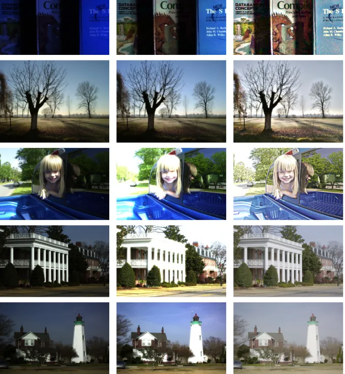
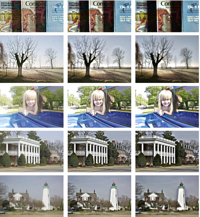
In Fig.4 we show a comparaison between the results of SLMRSR and SLMRACE with the
same kernel size of 25×25. It can be seen that images filtered with SLMRACE show much more
details than those filtered with SLMRSR without corrupting colors.
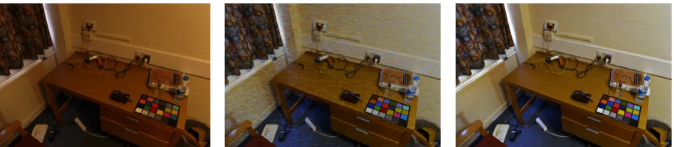
In Fig.5we present the influence of three kernel sizes on the results. It can be seen that a large
kernel size allows us to see more details and obtain an output image with more contrast. However,
with a large kernel size we can see a halo effect near the edges. Our tests have shown that the
intermediate choice of kernel size of 25 × 25 is a good trade-off.
5 Conclusions
In this paper we have recalled the so-called spray-based implementations of some Retinex-inspired
color correction algorithms and pointed out their limits: high computational time and noise
gen-eration. We have also discussed a recent proposal to avoid this kind of problems and showed
that it can be applied to RACE, the algorithm obtained from the fusion of RSR, the random spray
Retinex implementation, and the perceptually-inspired color correction model ACE. Finally, we
have presented tests and comparisons to corroborate the good performances of this new RACE
Fig 4 Left: original image. Middle: output of SLMRSR. Right: output of SLMRACE with a slope α = 2 and a number of spray pixel n equal to the integer part of the image diagonal of each image.
Acknowledgments
The authors would like to thank Nikola Bani´c for his help and advise during the implementation
Fig 5 Output of SLMRACE with different kernel sizes s Left: s = 5 × 5. Middle: s = 25 × 25. Right: s = 50 × 50.
References
1 E. Land and J. McCann, “Lightness and Retinex theory,” Journal of the Optical Society of
America61, 1–11 (1971).
between theoretical predictions and observer responses to the ‘color mondrian’ experiments,”
Journ. of Vision Res.16, 445–458 (1976).
3 J. Frankle and J. J. McCann, “Method and apparatus for lightness imaging.” United States
Patent, US 4,348,336 (1983).
4 D. Marini and A. Rizzi, “A computational approach to color adaptation effects,” Image and
Vision Computing18, 1005–1014 (2000).
5 T. J. Cooper and F. A. Baqai, “Analysis and extensions of the Frankle-McCann Retinex
algo-rithm,” Journal of Electronic Imaging 13, 85–92 (2004).
6 J. J. McCann and et al., “Special session on Retinex at 40,” Journal of Electronic Imaging 13,
6–145 (2004).
7 E. Provenzi, L. De Carli, A. Rizzi, and D. Marini, “Mathematical definition and analysis of
the retinex algorithm,” Journal of the Optical Society of America A 22, 2613–2621 (2005).
8 E. Provenzi, M. Fierro, A. Rizzi, L. De Carli, D. Gadia, and D. Marini, “Random spray
retinex: A new retinex implementation to investigate the local properties of the model,” IEEE
Transactions on Image Processing16, 162–171 (2007).
9 A. Rizzi, C. Gatta, and D. Marini, “A new algorithm for unsupervised global and local color
correction,” Pattern Recognition Letters 24, 1663–1677 (2003).
10 E. Provenzi, C. Gatta, M. Fierro, and A. Rizzi, “Spatially variant white patch and gray world
method for color image enhancement driven by local contrast,” IEEE Trans. on Pattern
Anal-ysis and Machine Intelligence30, 1757–1770 (2008).
11 N. Bani´c and S. Lonˇcari´c, “Light random sprays retinex: Exploiting the noisy illumination
12 N. Bani´c and S. Lonˇcari´c, “Smart light random memory sprays retinex: a fast retinex
im-plementation for high-quality brightness adjustment and color correction,” JOSA A 32(11),
2136–2147 (2015).
13 G. Buchsbaum, “A spatial processor model for object colour perception,” Journal of the
Franklin Institute310, 337–350 (1980).
List of Figures
1 A random spray used in RSR.
2 Left: original image. Right: output of RSR with N = 4 sprays and n = 5 pixels
per spray.
3 Left: original image. Middle: output of spray memory RSR without applying the
filters of LRSR. Right: output of SLMRSR.
4 Left: original image. Middle: output of SLMRSR. Right: output of SLMRACE
with a slope α = 2 and a number of spray pixel n equal to the integer part of the
image diagonal of each image.
5 Output of SLMRACE with different kernel sizes s Left: s = 5 × 5. Middle:
s = 25 × 25. Right: s = 50 × 50.