HAL Id: hal-00944098
https://hal.inria.fr/hal-00944098
Preprint submitted on 10 Feb 2014HAL is a multi-disciplinary open access archive for the deposit and dissemination of sci-entific research documents, whether they are pub-lished or not. The documents may come from
L’archive ouverte pluridisciplinaire HAL, est destinée au dépôt et à la diffusion de documents scientifiques de niveau recherche, publiés ou non, émanant des établissements d’enseignement et de
Influence functions for CART
Avner Bar Hen, Servane Gey, Jean-Michel Poggi
To cite this version:
Influence Functions for CART
Avner Bar-Hen
∗, Servane Gey
†, Jean-Michel Poggi
‡ AbstractThis paper deals with measuring the influence of observations on the results obtained with CART classification trees. To define the influence of individuals on the analysis, we use influence functions to propose some general criterions to measure the sensitivity of the CART analysis and its robustness. The proposals, based on jakknife trees, are organized around two lines: influence on predictions and influence on partitions. In addition, the analysis is extended to the pruned sequences of CART trees to produce a CART specific notion of influence.
A numerical example, the well known spam dataset, is presented to illustrate the notions developed throughout the paper. A real dataset relating the administrative classification of cities surrounding Paris, France, to the characteristics of their tax revenues distribution, is finally analyzed using the new influence-based tools.
1 Introduction
Classification And Regression Trees (CART; Breiman et al. (1984) [4]) have proven to be very useful in various applied contexts mainly because models can include numerical as well as nominal explanatory variables and because models can be easily represented (see for exam-ple Zhang and Singer (2010) [23], or Bel et al. (2009) [2]). Because CART is a nonparametric method as well as it provides data parti-tioning into distinct groups, such tree models have several additional
∗Laboratoire MAP5, Universit´e Paris Descartes & EHESP, Rennes, France †Laboratoire MAP5, Universit´e Paris Descartes, France
‡Laboratoire de Math´ematiques, Universit´e Paris Sud, Orsay, France and Universit´e
Paris Descartes, France
hal-00562039, version 1 - 2 Feb 201
advantages over other techniques: for example input data do not need to be normally distributed, predictor variables are not supposed to be independent, and non linear relationships between predictor variables and observed data can be handled.
It is well known that CART appears to be sensitive to perturbations of the learning set. This drawback is even a key property to make resam-pling and ensemble-based methods (as bagging and boosting) effective (see Gey and Poggi (2006) [10]). To preserve interpretability of the obtained model, it is important in many practical situations to try to restrict to a single tree. The stability of decision trees is then clearly an important issue and then it is important to be able to evaluate the sensitivity of the data on the results. Recently Briand et al. (2009) [5] propose a similarity measure between trees to quantify it and use it from an optimization perspective to build a less sensitive variant of CART. This view of instability related to bootstrap ideas can be also examined from a local perspective. Following this line, Bousquet and Elisseeff (2002) [3] studied the stability of a given method by replacing one observation in the learning sample with another one coming from the same model.
Classically, robustness is mainly devoted to model stability, considered globally, rather than focusing on individuals or using local stability tools (see Rousseeuw and Leroy (1987) [19] or Verboven and Huber (2005) [22] in the parametric context and Ch`eze and Poggi (2006) [7] for nonparametric context).
The aim of this paper is to focus on individual observations diagno-sis issues rather than model properties or variable selection problems. The use of an influence function is a classical diagnostic method to measure the perturbation induced by a single element, in other terms we examine stability issue through jackknife. We use decision trees to perform diagnosis on observations. Huber (1981) [13] used influence curve theory to define different classes of robust estimators and to de-fine a measure of sensitivity for usual estimators.
The outline is the following. Section 2 recalls first some general back-ground on the so-called CART method and some basic ideas about influence functions. Then it introduces some influence functions for CART based on predictions, or on partitions, and finally an influence function more deeply related to CART method involving sequences of pruned trees. Section 3 contains an illustrative numerical
applica-hal-00562039, version 1 - 2 Feb 201
tion on the spam dataset (see Hastie, Tibshirani and Friedman (2009) [12]). Section 4 explores an original dataset relating the administrative classification of cities surrounding Paris, France, to the characteristics of their tax revenues distribution, by using the new influence-based tools. Finally Section 5 opens some perspectives.
2 Methods and Notations
2.1 CART
Let us briefly recall, following Bel et al. [2], some general background on Classification And Regression Trees (CART). For more detailed presentation see Breiman et al. [4] or, for a simple introduction, see Venables and Ripley (2002) [21]. The data are considered as an inde-pendent sample of the random variables (𝑋1, . . . , 𝑋𝑝, 𝑌 ), where the
𝑋𝑘s are the explanatory variables and 𝑌 is the categorical variable to
be explained. CART is a rule-based method that generates a binary tree through recursive partitioning that splits a subset (called a node) of the data set into two subsets (called sub-nodes) according to the minimization of a heterogeneity criterion computed on the resulting sub-nodes. Each split is based on a single variable; some variables may be used several times while others may not be used at all. Each sub-node is then split further based on independent rules. Let us consider a decision tree 𝑇 . When 𝑌 is a categorical variable a class label is assigned to each terminal node (or leaf) of 𝑇 . Hence 𝑇 can be viewed as a mapping to assign a value ˆ𝑌𝑖 = 𝑇 (𝑋𝑖1, . . . , 𝑋𝑖𝑝) to each
sample. The growing step leading to a deep maximal tree is obtained by recursive partitioning of the training sample by selecting the best split at each node according to some heterogeneity index, such that it is equal to 0 when there is only one class represented in the node to be split, and is maximum when all classes are equally frequent. The two most popular heterogeneity criteria are the Shannon entropy and the Gini index. Among all partitions of the explanatory variables at a node 𝑡, the principle of CART is to split 𝑡 into two sub-nodes 𝑡−
and 𝑡+ according to a threshold on one of the variables, such that the reduction of heterogeneity between a node and the two sub-nodes is maximized. The growing procedure is stopped when there is no more admissible splitting. Each leaf is assigned to the most frequent class of its observations. Of course, such a maximal tree (denoted by 𝑇𝑚𝑎𝑥)
generally overfits the training data and the associated prediction error
hal-00562039, version 1 - 2 Feb 201
𝑅(𝑇𝑚𝑎𝑥), with
𝑅(𝑇 ) = ℙ{𝕋(𝕏⊮, . . . , 𝕏∣) ∕= 𝕐}, (1)
is typically large. Since the goal is to build from the available data a tree 𝑇 whose prediction error is as small as possible, in a second stage the tree 𝑇𝑚𝑎𝑥 is pruned to produce a subtree 𝑇′ whose expected
performance is close to the minimum of 𝑅(𝑇′) over all binary subtrees
𝑇′ of 𝑇
𝑚𝑎𝑥. Since the joint distribution ℙ of (𝑋1, . . . , 𝑋𝑝, 𝑌 ) is
un-known, the pruning is based on the penalized empirical risk ˆ𝑅𝑝𝑒𝑛(𝑇 )
to balance optimistic estimates of empirical risk by adding a complex-ity term that penalizes larger subtrees. More precisely the empirical risk is penalized by a complexity term, which is linear in the number of leaves of the tree:
ˆ 𝑅𝑝𝑒𝑛(𝑇 ) = 𝑛1 𝑛 ∑ 𝑖=1 1l𝑇 (𝑋1 𝑖,...,𝑋𝑖𝑝)∕=𝑌𝑖+ 𝛼∣𝑇 ∣ (2)
where 1l is the indicator function, 𝑛 the total number of samples and
∣𝑇 ∣ denotes the number of leaves of the tree 𝑇 .
The R package rpart provides both the sequence of subtrees pruned from a deep maximal tree and a final tree selected from this sequence by using the 1-SE rule (see [4]). The maximal tree is constructed by using the Gini index (default) and stops when the minimum number of observations in a leaf is reached, or if the misclassification rate of the branch provided by splitting a node is too small. The penalized criterion used in the pruning of rpart is ˆ𝑅𝑝𝑒𝑛 defined by (2). The
cost complexity parameter denoted by 𝑐𝑝 corresponds to the temper-ature 𝛼 used in the original penalized criterion (2) divided by the misclassification rate of the root of the tree. The pruning step leads to a sequence {𝑇1; . . . ; 𝑇𝐾} of nested subtrees (where 𝑇𝐾 is reduced
to the root of the tree) associated with a nondecreasing sequence of temperatures {𝑐𝑝1; . . . ; 𝑐𝑝𝐾}. Then, the selection step is based on
the 1-SE rule: using cross-validation, rpart computes 10 estimates of each prediction error 𝑅(𝑇𝑘), leading to average misclassification
er-rors { ˆ𝑅𝑐𝑣(𝑇1); . . . ; ˆ𝑅𝑐𝑣(𝑇𝐾)} and their respective standard deviations
{𝑆𝐸(𝑇1); . . . ; 𝑆𝐸(𝑇𝐾)}. Finally, the selected subtree corresponds to
the maximal index 𝑘1 such that ˆ
𝑅𝑐𝑣(𝑇𝑘1) ⩽ ˆ𝑅𝑐𝑣(𝑇𝑘0) + 𝑆𝐸(𝑇𝑘0),
where ˆ𝑅𝑐𝑣(𝑇𝑘0) = min1⩽𝑘⩽𝐾𝑅ˆ𝑐𝑣(𝑇𝑘).
hal-00562039, version 1 - 2 Feb 201
2.2 Influence function
We briefly recall some basics about influence functions. Let 𝑋1, . . . , 𝑋𝑛
be random variables with common distribution function (df) 𝐹 on ℝ𝑑
(𝑑 ≥ 1). Suppose that the parameter of interest is a statistic 𝑇 (𝐹 ) of the generating df, 𝑇 being defined at least on the space of df’s. The natural estimator is 𝑇 (𝐹𝑛) where 𝐹𝑛 is the empirical df, defined by
𝐹𝑛= 𝑛1
𝑛
∑
𝑖=1
𝛿𝑋𝑖
with 𝛿𝑋𝑖 the point mass 1 at 𝑋𝑖.
To evaluate the importance of an additional observation 𝑥 ∈ ℝ𝑑, we
can define, under conditions of existence, the quantity
𝐼𝐶𝑇,𝐹(𝑥) = lim𝜖→0𝑇
(
(1 − 𝜖)𝐹 + 𝜖 𝛿𝑥)− 𝑇(𝐹)
𝜖 (3)
which measures the influence of an infinitesimal perturbation along the direction 𝛿𝑥 (see Hampel (1988) [11]). The influence function (or
influence curve) 𝐼𝐶𝑇,𝐹(⋅) is defined pointwise by (3), if the limit exists
for every 𝑥.
There is strong connection between influence function and jackknife (see Miller (1974) [15]). Indeed, let 𝐹𝑛−1(𝑖) = 1
𝑛−1 ∑ 𝑗∕=𝑖𝛿𝑥𝑗, then 𝐹𝑛= 𝑛−1 𝑛 𝐹𝑛−1(𝑖) +1𝑛𝛿𝑥𝑖. If 𝜖 = −𝑛−11 , we have: 𝐼𝐶𝑇,𝐹𝑛(𝑥𝑖) ≈ 𝑇((1 − 𝜖)𝐹𝑛+ 𝜖 𝛿𝑥𝑖)− 𝑇(𝐹𝑛) 𝜖 (4) = (𝑛 − 1)(𝑇 (𝐹𝑛) − 𝑇 (𝐹𝑛−1(𝑖) )) = 𝑇∗ 𝑛,𝑖− 𝑇 (𝐹𝑛) (5)
where ≈ stands for asymptotic approximation, and the 𝑇∗
𝑛,𝑖 are the
pseudo-values of the jackknife (i.e. values computed on 𝑛 − 1 obser-vations) [15].
Influence analysis for discriminant analysis has been studied by Camp-bell (1978) [6], Critchley and Vitiello (1991) [8] for the linear case and Croux and Joossens (2005) [9] for the quadratic one. Extension to nonparametric supervised classification in not easy since it is difficult to obtain an exact form for 𝑇 (𝐹 ). In this article we will use jackknife as an estimate of the influence function.
hal-00562039, version 1 - 2 Feb 201
2.3 Influence functions for CART
In this section, we present different influence functions for CART. Let
𝑋 = (𝑋1, . . . , 𝑋𝑝) ∈ 𝒳 be the explanatory variable, and consider that
the data are some independent realization ℒ = {(𝑋1, 𝑌1); . . . ; (𝑋𝑛, 𝑌𝑛)}
of (𝑋, 𝑌 ) ∈ 𝒳 × {1; . . . ; 𝐽}. For a given tree 𝑇 = 𝑇 (ℒ), we denote any node of 𝑇 by 𝑡. Hence, we use the following notations:
∙ ˜𝑇 the set of leaves of 𝑇 , and ∣𝑇 ∣ the number of leaves of 𝑇 ,
∙ the empirical distribution p𝑥,𝑇 of 𝑌 conditionally to 𝑋 = 𝑥 and
𝑇 , is defined by: for 𝑗 = 1, . . . , 𝐽, p𝑥,𝑇(𝑗) = 𝑝(𝑗∣𝑡) the proportion
of the class 𝑗 in the leaf of 𝑇 in which 𝑥 falls.
We denote by 𝑇 the tree obtained from the complete sample ℒ, while (
𝑇(−𝑖))
1⩽𝑖⩽𝑛denote jackknife trees obtained from (ℒ ∖ {(𝑋𝑖, 𝑌𝑖)})1⩽𝑖⩽𝑛. For a given tree 𝑇 , two different main aspects are of interest: the predictions delivered by the tree or the partition associated with the tree, the second highlights the tree structure while the first focuses on its predictive performance. This distinction is classical and already examined for example by Miglio and Soffritti (2004) [14] recalling some proximity measures between classification trees and promoting the use of a new one mixing the two aspects. We then derive two kinds of influence functions for CART based on jackknife trees: influence on predictions and influence on partitions. In addition, the analysis is extended to the pruned sequences of CART trees to produce a CART specific notion of influence.
2.3.1 Influence on predictions
We propose three influence functions based on predictions.
The first, closely related to the resubstitution estimate of the tion error, evaluates the impact of a single change on all the predic-tions, is defined by: for 𝑖 = 1, . . . , 𝑛
𝐼1(𝑥𝑖) =
𝑛
∑
𝑘=1
1l𝑇 (𝑥𝑘)∕=𝑇(−𝑖)(𝑥𝑘), (6)
i.e. 𝐼1(𝑥𝑖) is the number of observations for which the predicted label
changes using the jackknife tree 𝑇(−𝑖) instead of the reference tree 𝑇 . The second, closely related to the leave-one-out estimate of the pre-diction error, is: for 𝑖 = 1, . . . , 𝑛
𝐼2(𝑥𝑖) = 1l𝑇 (𝑥𝑖)∕=𝑇(−𝑖)(𝑥𝑖), (7)
hal-00562039, version 1 - 2 Feb 201
i.e. 𝐼2(𝑥𝑖) indicates if 𝑥𝑖 is classified in the same way by 𝑇 and 𝑇(−𝑖).
The third one measures the distance between the distribution of the label in the nodes where 𝑥𝑖 falls: for 𝑖 = 1, . . . , 𝑛
𝐼3(𝑥𝑖) = 𝑑
(
p𝑥𝑖,𝑇, p𝑥𝑖,𝑇(−𝑖)
)
, (8)
where 𝑑 is a distance (or a divergence) between probability distribu-tions.
𝐼1 and 𝐼2 are based on the predictions only while 𝐼3 is based on the distribution of the labels in each leaf.
To compute 𝐼3, several distances or divergences can be used. In this paper, we use the total variation distance: for 𝑝 and 𝑞 two distribu-tions on {1; . . . ; 𝐽}, 𝑑(𝑝, 𝑞) = max 𝐴⊂{1;...;𝐽}∣𝑝(𝐴) − 𝑞(𝐴)∣ = 2 −1∑𝐽 𝑗=1 ∣𝑝(𝑗) − 𝑞(𝑗)∣
Remark 1. The Kullback-Leibler divergence (relied to the Shannon entropy index) and the Hellinger distance (relied to the Gini index) can also be used instead of the total variation distance.
2.3.2 Influence on partitions
We propose two influence functions based on partitions: 𝐼4 measuring the variations on the number of clusters in each partition, and 𝐼5based on the quantification of the difference between the two partitions. These indices are computed in the following way: for 𝑖 = 1, . . . , 𝑛
𝐼4(𝑥𝑖) = ∣𝑇(−𝑖)∣ − ∣𝑇 ∣, (9)
𝐼5(𝑥𝑖) = 1 − 𝐽
( ˜
𝑇 , ˜𝑇(−𝑖)), (10)
where 𝐽(𝑇 , ˜˜ 𝑇(−𝑖))is the Jaccard dissimilarity between the partitions of ℒ respectively defined by ˜𝑇(−𝑖) and ˜𝑇 .
Recall that, for two partitions 𝐶1 and 𝐶2 of ℒ, the Jaccard coefficient
𝐽(𝐶1, 𝐶2) is computed as
𝐽(𝐶1, 𝐶2) = 𝑎 + 𝑏 + 𝑐𝑎 ,
hal-00562039, version 1 - 2 Feb 201
where 𝑎 counts the number of pairwise points of ℒ belonging to the same cluster in both partitioning, 𝑏 the number of pairwise points be-longing to the same cluster in 𝐶1, but not in 𝐶2, and 𝑐 the number of pairwise points belonging to the same cluster in 𝐶2, but not in 𝐶1. The more similar 𝐶1 and 𝐶2, the closer 𝐽(𝐶1, 𝐶2) to 1.
Remark 2. Such influence index can be generated using different dissimilarities between partitions. For a detailed analysis and com-parisons, see [20].
2.3.3 Influence based on subtrees sequences
Another way to inspect the dataset is to consider the complexity cost constant, penalizing bigger trees in the pruning step of the CART tree design, as a tuning parameter. It allows to scan the data and sort them with respect to their influence on the CART tree.
Let us consider on the one hand the sequence of subtrees based on the complete dataset, denoted by 𝑇 , and on the other hand the 𝑛 jackknife sequences of subtrees based on the jackknife subsamples ℒ∖{(𝑋𝑖, 𝑌𝑖)},
denoted by 𝑇(−𝑖)(𝑖 = 1, . . . , 𝑛). Suppose that the sequence 𝑇 contains
𝐾𝑇 elements, and that each sequence 𝑇(−𝑖) contains 𝐾𝑇(−𝑖) elements
(𝑖 = 1, . . . , 𝑛). This leads to a total of 𝑁𝑐𝑝 ⩽ 𝐾𝑇 +∑1⩽𝑖⩽𝑛𝐾𝑇(−𝑖)
distinct values {𝑐𝑝1; . . . ; 𝑐𝑝𝑁𝑐𝑝} of the cost complexity parameter in
in-creasing order from 𝑐𝑝1= 0.01 (the default value in rpart) to 𝑐𝑝𝑁𝑐𝑝=
max1⩽𝑗⩽𝑁𝑐𝑝𝑐𝑝𝑗.
Then, for each value 𝑐𝑝𝑗 of the complexity and each observation 𝑥𝑖,
we compute the binary variable 1l𝑇
𝑐𝑝𝑗(𝑥𝑖)∕=𝑇𝑐𝑝𝑗(−𝑖)(𝑥𝑖) that tells us if the
reference and jackknife subtrees corresponding to the same complexity
𝑐𝑝𝑗 provide different predicted labels for the removed observation 𝑥𝑖.
Thus we define influence function 𝐼6 as the number of complexities for which these predicted labels differ: for 𝑖 = 1, . . . , 𝑛
𝐼6(𝑥𝑖) = 𝑁𝑐𝑝 ∑ 𝑗=1 1l𝑇 𝑐𝑝𝑗(𝑥𝑖)∕=𝑇𝑐𝑝𝑗(−𝑖)(𝑥𝑖). (11)
Remark 3. Since the jackknife sequences of subtrees do not change for many observations, usually we obtain that 𝑁𝑐𝑝<< 𝐾𝑇+∑1⩽𝑖⩽𝑛𝐾𝑇(−𝑖).
hal-00562039, version 1 - 2 Feb 201
3 Illustration on Spam Dataset
3.1 Spam dataset
The spam data (The data are publicly available at ftp.ics.uci.edu. consists of information from 4601 email messages, in a study to screen email for ”spam” (i.e. junk email). The data are presented in details in [12, p. 301]. The response variable is binary, with values nonspam or spam, and there are 57 predictors: 54 given by the percentage of words in the email that match a given word or a given character, and three related to uninterrupted sequences of capital letters: the average length, the length of the longest one and the sum of the lengths of uninterrupted sequences. The objective was to design an automatic spam detector that could filter out spam before clogging the users’ mailboxes. This is a supervised learning problem.
3.2 Reference tree and jackknife trees
The reference tree is obtained using the R package rpart (see [16], [21]) and accepting the default values for all the parameters (mainly the Gini heterogeneity function to grow the maximal tree and pruning thanks to 10-fold cross-validation).
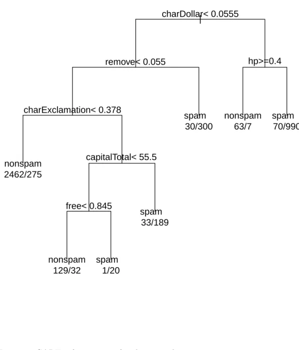
The reference tree based on all observations, namely 𝑇 , is given in Figure 1. This tree has 7 leaves, obtained from splits involving the variables 𝑐ℎ𝑎𝑟𝐷𝑜𝑙𝑙𝑎𝑟, 𝑟𝑒𝑚𝑜𝑣𝑒, ℎ𝑝, 𝑐ℎ𝑎𝑟𝐸𝑥𝑐𝑙𝑎𝑚𝑎𝑡𝑖𝑜𝑛, 𝑐𝑎𝑝𝑖𝑡𝑎𝑙𝑇 𝑜𝑡𝑎𝑙, and 𝑓𝑟𝑒𝑒 (in order of appearance in the tree). Each leaf is labeled by the prediction of 𝑌 (spam or nonspam) and the distribution of 𝑌 inside the node (for example, the third leaf is almost pure: it contains 1 nonspam and 20 spams). These make the tree easy to interpret and to describe: indeed, from the direct interpretation of the path from the root to the third leaf, an email containing many occurrences of ”$”, ”!”, ”remove”, capital letters and ”free” is almost always a spam. To compute the influence of one observation we compute 𝑇(−𝑖)the tree based on all observations except the observation 𝑖 (𝑖 = 1, . . . , 4601). We then obtain a collection of 4601 trees, which can be described with respect to the reference tree 𝑇 in many different ways. This descrip-tion is carried out according to various filters, namely: the retained variables, the number of leaves of the final tree, the observations in-volved in the differences. The variables charDollar, charExclamation,
hal-00562039, version 1 - 2 Feb 201
|
charDollar< 0.0555
remove< 0.055
charExclamation< 0.378
capitalTotal< 55.5
free< 0.845
hp>=0.4
nonspam
2462/275
nonspam
129/32
spam
1/20
spam
33/189
spam
30/300
nonspam
63/7
spam
70/990
Figure 1: CART reference tree for the spam dataset.
hal-00562039, version 1 - 2 Feb 201
hp and remove are always present. The variable capitalLong is present
in 88 trees, the variable capitalTotal is present in 4513 trees and the variable free is present in 4441 trees. This indicates instable clades within 𝑇 . In addition variables free and capitalLong as well as
capi-talLong and capitalTotal never appear simultaneously, while the 4441
trees containing free also contain capitalTotal. This highlights the variability among the 4601 trees. All the differences are explained by the presence (or not) of the variable free. Indeed, removing one ob-servation from node 8 is enough to remove the split generated from variable free and to merge the two nodes leading to misclassification. There are 77 observations 𝑥𝑖 classified differently by 𝑇 and the
cor-responding jackknife tree 𝑇(−𝑖), and 160 jackknife trees with one less leaf than 𝑇 . All the other jackknife trees have the same number of leaves as 𝑇 . The indices of the aforesaid observations are given in Table 5 of the appendix. Denoting by DC the set of indices 𝑖 for which 𝑥𝑖 is classified differently by 𝑇 and 𝑇(−𝑖), and by DNF the set
of indices 𝑖 for which 𝑇(−𝑖) has one less leaf than 𝑇 , let us empha-size that the cardinality of DC∪DNF is equal to 162, which means that two observations are classified differently, but lead to jackknife trees having the same number of leaves as 𝑇 . A careful examination of the highlighted observations leads to a spam and a nonspam mails that define the second split of the reference tree: the threshold on the variable remove is the middle of their corresponding values.
3.3 Influence functions
The influence functions 𝐼1, 𝐼2, 𝐼3, 𝐼4, 𝐼5 and 𝐼6 respectively defined by (6), (7), (8), (9), (10) and (11) are computed on the spam dataset by using the jackknife trees computed in paragraph 3.2. The results are summarized in the following paragraphs.
3.3.1 Influence on predictions
Indices 𝐼1and 𝐼3computed on the 163 observations of the spam dataset for which 𝐼1 is nonzero are given in Figure 2.
There are 77 observations for which 𝐼2 = 1, that is for which 𝑥𝑖 is
classified differently by 𝑇 and the corresponding jackknife tree 𝑇(−𝑖), while 163 jackknife trees lead to a nonzero number of observations for which the predicted label changes. These observations correspond to observations leading to jackknife trees sufficiently perturbed from
hal-00562039, version 1 - 2 Feb 201
0 1000 2000 3000 4000 0 20 40 60 80 Influence function I1 Observations indices Number of obser v ations diff erently labeled 0 1000 2000 3000 4000 0.0 0.2 0.4 0.6 0.8 Influence function I3 Observations indices T otal v ar iation distance
Figure 2: Influence indices based on predictions for the spam dataset.
𝑇 to have a different shape. The 77 aforesaid observations lead to
a total variation distance between p𝑥𝑖,𝑇 and p𝑥𝑖,𝑇(−𝑖) larger than 0.6.
The others lead to a total variation distance smaller than 0.1. The 86 remaining jackknife trees for which the number of observations differ-ently labeled is nonzero provide total variation distances from 0.016 to 0.1.
𝐼1 and 𝐼2 are based on the predictions only while 𝐼3 takes into account the distribution of the labels in each leaf. For example, the contribu-tion of 𝐼3 with respect to 𝐼2 is that some observations are classified similarly by 𝑇 and 𝑇(−𝑖), but actually lead to conditional probability distributions p𝑥𝑖,𝑇(−𝑖) largely different from p𝑥𝑖,𝑇. These observations
are not sufficiently important in the construction of 𝑇 to perturb the classification, but play some role in the tree instability.
3.3.2 Influence on partitions
Influence index 𝐼5 on the 160 observations of the spam dataset for which the jackknife tree has one leaf less than 𝑇 is given in Figure 3. There are 160 jackknife trees having one less leaf than 𝑇 , and 163 leading to a partition ˜𝑇(−𝑖) different from ˜𝑇 . Among the 160
afore-hal-00562039, version 1 - 2 Feb 201
0 1000 2000 3000 4000 0.00 0.01 0.02 0.03 0.04 0.05 0.06 Influence function I5 Observations indices Dissimilar ity
Figure 3: Influence index based on partitions for the spam dataset.
said trees, 139 lead to a partition ˜𝑇(−𝑖) of dissimilarity larger than 0.05. Hence there are 21 trees with one less leaf than 𝑇 , but leading to a partition ˜𝑇(−𝑖) not far from ˜𝑇 . The others perturb sufficiently
𝑇 to change the partition consequently. Let us note that all jackknife
trees partitions are of dissimilarity smaller than 0.06 from ˜𝑇 . This is
due to the very local perturbations around 𝑥𝑖.
Let us emphasize that the 163 trees leading to a partition ˜𝑇(−𝑖) differ-ent from ˜𝑇 correspond exactly to the 163 trees leading to a nonzero
number of mails classified differently. This shows an unexpected be-havior of CART on this dataset: different partitions lead to predictors assigning different labels on the training sample.
3.3.3 Influence based on subtrees sequences
The pruned subtrees sequences contain around six elements and they represent 𝑁𝑐𝑝= 27 distinct values {𝑐𝑝1; . . . ; 𝑐𝑝27} of the cost complex-ity parameter (from 0.01 to 0.48).
The distribution of influence index 𝐼6 is given in Table 1.
hal-00562039, version 1 - 2 Feb 201
𝐼6 0 1 2 3 4 7 12 13 14 17 18 21
Nb. Obs. 2768 208 1359 79 62 1 1 66 30 2 23 2 Table 1: Frequency distribution of the influence index 𝐼6 over the 4601 emails.
The number of actual values of 𝐼6 is small. These values organize the data as nested level sets in decreasing order of influence. For 60% of the observations, predictions are the same all along the pruned subtrees sequences, making these observations not influential for 𝐼6. There are 123 observations leading to different predictions for at least half of the pruned subtrees, and only 2 observations lead to 77.8% of the complexity values for which predicting labels change. Let us remark that these two most influential mails for 𝐼6 are the same mails influential for 𝐼2 and 𝐼4 given in Table 5.
Index 𝐼6 can be examined in a structural way by locating the ob-servation on the topology of the reference tree. Of course, graphical software tools based on such idea can be useful to screen a given data set.
Remark 4. Let us recall that the influence is measured with respect to a reference model and of course more instable reference tree auto-matically increases the number of individuals that can be categorized as influential. In fact, even if it is implicit, influence functions are rela-tive to a given model. Typically, increasing the number of leaves of the reference tree automatically promotes new observations as influential.
4 Exploring the Paris Tax Revenues
dataset
4.1 Dataset and reference tree
4.1.1 Dataset
We apply the tools presented in the previous section on tax revenues of households in 2007 from the 143 cities surrounding Paris. Cities are grouped into four counties (corresponding to the french administrative “d´epartement”). The PATARE data (PAris TAx REvenues) are freely available on http://www.data-publica.com/data. For confidential-ity reason we do not have access to the tax revenues of the individual
hal-00562039, version 1 - 2 Feb 201
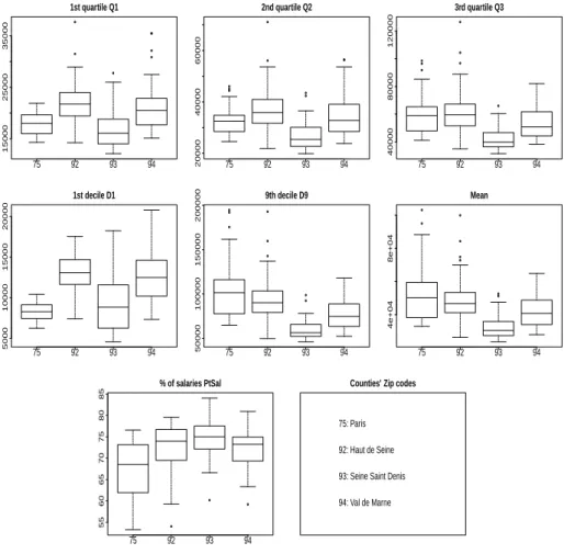
households but we have characteristics of the distribution of the tax revenues per city. Paris has 20 ”arrondissements” (corresponding to districts), Seine-Saint-Denis is located at the north of Paris and has 40 cities, Hauts-de-Seine is located at the west of Paris and has 36 cities, and Val-de-Marne is located at the south of Paris and has 48 cities. For each city, we have the first and the 9th deciles (named respectively D1 and D9), the quartiles (named respectively Q1, Q2 and Q3), the mean, and the percentage of the tax revenues coming from the salaries and treatments (named PtSal). Figure 4 gives the summary statistics for each variable per county.
75 92 93 94 15000 25000 35000 1st quartile Q1 75 92 93 94 20000 40000 60000 2nd quartile Q2 75 92 93 94 40000 80000 120000 3rd quartile Q3 75 92 93 94 5000 10000 15000 20000 1st decile D1 75 92 93 94 50000 100000 150000 200000 9th decile D9 75 92 93 94 4e+04 8e+04 Mean 75 92 93 94 55 60 65 70 75 80 85
% of salaries PtSal Counties’ Zip codes
75: Paris 92: Haut de Seine 93: Seine Saint Denis 94: Val de Marne
Figure 4: PATARE dataset: boxplots of the variables per county (“d´epartement” in France) and zip codes for counties.
hal-00562039, version 1 - 2 Feb 201
Basically we tried to predict the county of the city with the characteris-tics of the tax revenues distribution. This is a supervised classification problem where the explained variable is quaternary.
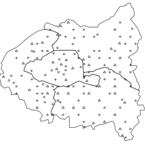
We emphasize that this information cannot be easily retrieved from the explanatory variables considered without the county information. Indeed, the map (see Figure 5) of the cities drawn according to a
𝑘-means (𝑘=4) clustering (each symbol is associated with a cluster)
superimposed with the borders of the counties, exhibits a poor recov-ery of counties through clusters.
Figure 5: Spatial representation of 𝑘-means (𝑘=4) clustering of the PATARE dataset cities (each symbol is associated with a cluster).
4.1.2 Reference tree
Figure 6 shows the reference tree. Each leaf is labelled by two infor-mations: the predicted county and the distribution of the cities over the 4 counties. For example the second leaf gives 0/17/1/3 meaning
hal-00562039, version 1 - 2 Feb 201
that it contains 0 districts from Paris, 17 cities from Hauts-de-Seine, 1 from Seine-Saint-Denis and 3 from Val-de-Marne.
All the 5 terminal nodes located on the left subtree below the root are homogeneous since the distributions are almost pure, while half the nodes of the right subtree are highly heterogeneous. The first split in-volves the last decile of the income distribution and then discriminates the rich cities concentrated in the left part from the others. Accord-ing to this first split, the labels distAccord-inguish Paris and Hauts-de-Seine on the left from Seine-Saint-Denis on the right, while Val-de-Marne appears in both sides.
The extreme quantiles are sufficient to separate richest from poorest counties while more global predictors are useful to further discrimi-nate between intermediate cities. Indeed the splits on the left part are mainly based on the deciles D1, D9 and PtSal is only used to sepa-rate Hauts-de-Seine from Val-de-Marne. The splits on the right part are based on all the dependent variables but involve PtSal and mean variables to separate Seine-Saint-Denis from Val-de-Marne.
Surprisingly, the predictions given by the reference tree are generally correct (the resubstitution misclassification rate calculated from the confusion matrix given in Table 2, is equal to 24.3%). Since the cities within each county are very heterogeneous, we look for the cities which perturb the reference tree.
.
````````````
```
Actual Predicted Paris Haut de Seine Seine Saint Denis Val de Marne
Paris 20 0 0 0
Haut de Seine 0 30 1 5
Seine Saint Denis 1 4 28 7
Val de Marne 3 9 5 30
Table 2: Confusion matrix: actual versus predicted county, using the CART reference tree.
After this quick inspection of the reference tree avoiding careful in-spection of the cities inside the leaves, let us focus on the influential cities highlighted by the previously defined indices. In the sequel the cities (which are the individuals) are written in italics to be clearly dis-tinguished from counties which are written between quotation marks.
hal-00562039, version 1 - 2 Feb 201
4.2 Influential observations
4.2.1 Presentation
There are 45 cities classified differently by 𝑇 and the corresponding jackknife tree 𝑇(−𝑖), and 44 jackknife trees having a different number of leaves than 𝑇 . The frequency distribution of the difference in the number of leaves, summarized by the influence index 𝐼4, is given in Table 3. The aforesaid cities are given in Table 6 of the appendix, classified by their respective labels in the dataset. DC denotes the set of cities classified differently by 𝑇 and 𝑇(−𝑖), and DNF denotes the set of cities for which 𝑇(−𝑖) has not the same number of leaves as
𝑇 . Let us emphasize that the cardinality of DC∪DNF is equal to 63:
19 cities are classified differently by trees having the same number of leaves, while 18 cities lead to jackknife trees having different number of leaves, but classifying the corresponding cities in the same way.
𝐼4 -3 -2 -1 0 1
Nb. Obs. 1 8 25 99 10
Table 3: Frequency distribution of the influence index 𝐼4 over the 143 cities. Indices 𝐼1 and 𝐼3 computed on the 75 observations of the PATARE dataset for which 𝐼1 is nonzero are given in Figure 7.
There are 44 observations classified differently by 𝑇 and 𝑇(−𝑖), while 75 jackknife trees lead to a nonzero number of observations for which predicted labels change. These 75 jackknife trees contain the 63 trees for which the number of leaves changes or classifying the correspond-ing city differently. There are 13 cities for which the total variation distance between the distributions defined by 𝑇 and 𝑇−(𝑖)respectively
is larger than 0.5. Among these 13 cities, 2 lead to jackknife trees at distance 1 from 𝑇 : Asnieres sur Seine (from “Hauts-de-Seine”) and
Paris 13eme (from “Paris”). The value of 𝐼1 and 𝐼2 at these 2 points is
equal to 1, meaning that each city provides a jackknife tree sufficiently close to 𝑇 to unchange the classification, except for the removed city. In fact, if we compare the 2 jackknife trees with 𝑇 , we can notice that the thresholds in the second split for Asnieres sur Seine, and in the first split for Paris 13eme, are slightly moved. It suffices to classify on the one hand Asnieres sur Seine in the pure leaf “Paris”, and on
hal-00562039, version 1 - 2 Feb 201
the other hand to remove Paris 13eme from this leaf to classify it in “Seine-Saint-Denis”. This explains the astonishing value of 1 for the corresponding total variation distances.
Influence index 𝐼5 on the 45 observations of the PATARE dataset for which 𝐼4 is nonzero is given in Figure 8.
There are 45 observations leading to jackknife trees having number of leaves different from 𝑇 . Two cities lead to jackknife trees providing partitions at distance larger than 0.5 from 𝑇 : Neuilly Plaisance and
Villemomble (both from “Seine-Saint-Denis”). When removed, these
2 cities change drastically the value of the threshold in the first split, what implies also drastic changes in the rest of the tree. Moreover, the corresponding jackknife trees have 2 less leaves than 𝑇 , what ob-viously increases the Jaccard distance between 𝑇 and each jackknife tree.
The frequency distribution of influence index 𝐼6 over the 143 cities of the PATARE dataset is given in Table 4.
𝐼6 0 1 2 3 4 6 7 9 10 12 13 14 16 17 21 24 26
Nb. Obs. 7 44 10 17 9 2 14 5 1 3 3 10 7 6 2 1 2 Table 4: Frequency distribution of influence index 𝐼6 over the 143 cities.
There are 29 different values of complexities in the reference and jac-cknife trees sequences. Two cities change prediction labels of trees for 26 complexities: Asnieres-sur-Seine and Villemomble. In the de-creasing order of influence, one city changes labels of trees for 24 complexities, and 2 cities for 21 complexities: Paris 13eme, and
Bry-sur-Marne (from “Val-de-Marne”), Rueil-Malmaison (from
“Hauts-de-Seine”). These 5 observations change labels for more than 72.4% of the complexities. 61 observations change labels of trees for less than 6.9% of the complexities.
Let us notice that Asnieres-sur-Seine and Paris 13eme have already been selected as influential for 𝐼3, and Villemomble for 𝐼5. Never-theless, the behaviours of 𝐼1, 𝐼2 and 𝐼3 at points Bry-sur-Marne and
Rueil-Malmaison are comparable to behaviours at points
Asnieres-sur-Seine and Paris 13eme: 𝐼1 and 𝐼2 are equal to 1, and 𝐼3 is equal
to 0.66, meaning that these 2 cities belong to the 13 cities for which
hal-00562039, version 1 - 2 Feb 201
𝐼3 is larger than 0.5. Let us also remark that only Montreuil (from “Seine-Saint-Denis”) is among the 13 aforesaid cities, but not in the 26 cities listed above and selected as influential for 𝐼4 and 𝐼6. The value of 𝐼3 at this point is equal to 0.52.
4.2.2 Interpretation
One can find in Figure 9 the influential cities, with respect to the two indices 𝐼4 and 𝐼6, located in the reference tree. Let us notice that most of the selected cities have also been selected by influence indices
𝐼1, 𝐼2, 𝐼3 and 𝐼5, so we refer only to 𝐼4 and 𝐼6 in what follows. Let us emphasize that only three cities among the 26 influential cities quoted in Figure 9 are misclassified when using the reference tree. Index 𝐼4 highlights cities (Noisy-le-Grand, Bagneux, Le Blanc
Mes-nil, Le Bourget, Neuilly-Plaisance, Noisy-le-Sec, Sevran, Vaujours and Villemomble) far from Paris and of middle or low social level. All the
cities having an index of -3 or -2 are located in nodes of the right part of the reference tree whereas the rich cities are concentrated in the left part.
Index 𝐼6 highlights cities for which two parts of the city can be distin-guished: a popular one with a low social level and a rich one of high social level. They are located in the right part of the reference tree (for the higher values of 𝐼6= 26, 24 and 21: Asnieres sur Seine,
Ville-momble, Paris 13eme, Bry-sur-Marne and Rueil-Malmaison) as well
as in the left part (for moderate values of 𝐼6 = 16 and 17:
Chatenay-Malabry, Clamart, Fontenay aux Roses, Gagny, Livry-Gargan, Vanves, Chevilly-Larue, Gentilly, Le Perreux sur Marne, Le Pre-Saint-Gervais, Maisons-Alfort, Villeneuve-le-Roi, Vincennes and the particularly
in-teresting city Villemomble for 𝐼6 = 26). Indeed, we can notice that only Villemomble is highlighted both by 𝐼4 and 𝐼6.
To explore the converse, we inspect now the list of the 51 cities as-sociated with lowest values of 𝐼6 (0 and 1) which can be considered as the less influential, the more stable. It can be easily seen that it corresponds to the 16 rich district of Paris downtown (Paris 1er to
12eme and Paris 14eme to Paris 16eme) and mainly cities near Paris
or directly connected by the RER line transportation.
It should be noted that the influence indices cannot be easily explained neither by central descriptors like the mean or the median Q2 nor by
hal-00562039, version 1 - 2 Feb 201
dispersion descriptors as Q3-Q1 and D9-D1. Bimodality seems the key property to explain high values of the influence indices.
In addition, coming back to the non supervised analysis, one may no-tice that influential observations for PCA are not related to influential cities detected using 𝐼6 index. Indeed, Figure 10 contains the two first principal components capturing more than 95% of the total variance. Each city is represented in this plane by a symbol of size proportional to the 𝐼6 index. Hence one can see that the points influential for PCA (those far from the origin) are generally of small influence for influence index 𝐼6.
4.2.3 Spatial interpretation
To end this study, a map is useful to capture the spatial interpreta-tion and complement the previous comments which need some prior knowledge about the sociology of the Paris area. In Figure 11, the 143 cities are represented by a circle proportional to the influence index
𝐼6 and a spatial interpolation is performed using 4 grey levels. This map shows that Paris is stable, and that each surrounding county contains a stable area: the richest or the poorest cities. What is remarkable is that the white as well as the gray areas are clustered.
5 Perspectives
Two directions for future work can be sketched.
First, the tools developed in this paper for the classification case can be generalized for the regression case. The instability is smoother in the regression case since the data are adjusted thanks to a sur-face rather than a frontier. Then the number of false classifications is replaced with the sum of square residuals typically which is more sen-sitive to perturbations but the differences between the full tree and the jackknife ones are more stringent in the classification case. Some clas-sical problems, like outlier detection has been intensively studied in the regression case and a lot of solutions have been developed around the ideas of robust regression (see Rousseeuw (1984) [18]). A com-plete scheme for comparison can be retrieved from Ch`eze and Poggi [7], where a tree-based algorithm has been developed and compared
hal-00562039, version 1 - 2 Feb 201
DNF∩DC DNF∖DC DC∖DNF 17 23 32 37 42 43 83 84 108 145 155 256 348 424 465 653 760 831 892 920 1071 1083 1114 1147 1151 1193 1195 1202 1207 1208 1213 1228 1231 1232 1258 1291 1292 1293 1389 1395 1401 1413 1458 1463 1466 1582 1602 1603 1631 1634 2158 2221 2303 2354 2356 2387 2711 2909 3090 3092 3272 3298 3453 3554 4068 4197 4211 4222 4230 4245 4392 4460 4462 4465 4492 486 1275 1823 1830 1841 1853 1862 1863 1866 1888 1942 1950 2069 2086 2114 2239 2340 2347 2365 2367 2434 2496 2615 2622 2645 2681 2696 2723 2792 2868 2880 2884 2885 3073 3085 3386 3420 3447 3460 3470 3701 3704 3807 3964 3967 3980 4038 4046 4061 4062 4067 4078 4083 4085 4093 4101 4102 4110 4112 4115 4124 4186 4224 4227 4232 4246 4247 4337 4341 4349 4366 4384 4391 4394 4396 4400 4401 4403 4454 4464 4473 4478 4502 4505 4594 1019 2987
Table 5: DNF : indices 𝑖 of observations from the spam dataset for which the corresponding jackknife tree 𝑇(−𝑖) has one less leaf than CART reference
tree 𝑇 . DC : indices 𝑖 for which 𝑥𝑖 is classified differently by 𝑇 and 𝑇(−𝑖).
intensively to well known competitive methods including robust re-gression.
Another direction is to focus on model stability and robustness rather than centering the analysis around individuals. A first idea could be, following Bar-Hen et al. (2008) [1], to build the most robust tree by iteratively remove the most influential observation until stabilisation between reference and jakknife trees. A second one is to consider, starting from the 𝐼6 index but summing on the observations instead of the complexities, the percentage of observations differently classified by the reference and jakknife subtrees at fixed complexity. This is out of the scope of this article.
6 Appendix
In Table 5 one can find three sets of indices for the spam dataset observations for which the jackknife tree differs from the reference tree.
hal-00562039, version 1 - 2 Feb 201
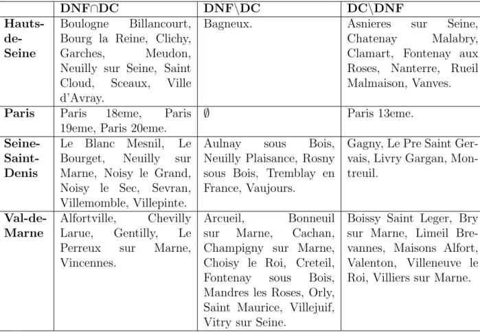
In Table 6 one can find, for each county, three sets of cities for the PATARE dataset for which the jackknife tree differs from the reference tree. DNF∩DC DNF∖DC DC∖DNF Hauts- de-Seine Boulogne Billancourt, Bourg la Reine, Clichy, Garches, Meudon, Neuilly sur Seine, Saint Cloud, Sceaux, Ville d’Avray.
Bagneux. Asnieres sur Seine, Chatenay Malabry, Clamart, Fontenay aux Roses, Nanterre, Rueil Malmaison, Vanves.
Paris Paris 18eme, Paris
19eme, Paris 20eme. ∅ Paris 13eme.
Seine- Saint-Denis
Le Blanc Mesnil, Le Bourget, Neuilly sur Marne, Noisy le Grand, Noisy le Sec, Sevran, Villemomble, Villepinte.
Aulnay sous Bois, Neuilly Plaisance, Rosny sous Bois, Tremblay en France, Vaujours.
Gagny, Le Pre Saint Ger-vais, Livry Gargan, Mon-treuil.
Val-de-Marne Alfortville,Larue, Gentilly,ChevillyLe
Perreux sur Marne, Vincennes.
Arcueil, Bonneuil sur Marne, Cachan, Champigny sur Marne, Choisy le Roi, Creteil, Fontenay sous Bois, Mandres les Roses, Orly, Saint Maurice, Villejuif, Vitry sur Seine.
Boissy Saint Leger, Bry sur Marne, Limeil Bre-vannes, Maisons Alfort, Valenton, Villeneuve le Roi, Villiers sur Marne.
Table 6: DNF: for the 4 counties, cities from the PATARE dataset for which the corresponding jackknife tree 𝑇(−𝑖) has not the same number of leaves as
CART reference tree 𝑇 . DC: cities classified differently by 𝑇 and 𝑇(−𝑖).
References
[1] Bar-Hen, A., Mariadassou, M., Poursat, M.-A. and Vandenkoorn-huyse, Ph. (2008).Influence Function for Robust Phylogenetic
Re-constructions. Molecular Biology and Evolution, 25(5), 869-873.
hal-00562039, version 1 - 2 Feb 201
[2] Bel, L., Allard, D., Laurent, J.M., Cheddadi, R. and Bar-Hen, A. (2009). CART algorithm for spatial data: application to
envi-ronmental and ecological data. Computat. Stat. and Data Anal.,
53(8), 3082-3093.
[3] Bousquet, O., Elisseeff, A. (2002). Stability and generalization. J. Machine Learning Res. 2, 499–526.
[4] Breiman, L., Friedman, J.H., Olshen, R.A. and Stone, C.J.
Clas-sification and regression trees. Chapman & Hall (1984).
[5] Briand, B., Ducharme, G. R., Parache, V. and Mercat-Rommens, C. (2009). A similarity measure to assess the stability of
classifi-cation trees, Comput. Stat. Data Anal., 53(4), 1208–1217.
[6] Campbell, N.A. (1978). The influence function as an aid in
out-lier detection in discriminant analysis., Appl. Statist., 27, 251–
258.
[7] Ch`eze, N. and Poggi, J.M. (2006). Outlier detection by boosting
regression trees. Journal of Statistical Research of Iran (JSRI), 3,
1–21.
[8] Critchley, F. and Vitiello, C. (1991). The influence of observations
on misclassification probability estimates in linear discriminant analysis., Biometrika, 78, 677–690.
[9] Croux, C. and Joossens, K. (2005). Influence of observations on
the misclassification probability in quadratic discriminant analy-sis., Journal of Multivariate Analysis, 96(2), 384–403.
[10] Gey, S. and Poggi, J.M. (2006). Boosting and instability for
re-gression trees. Comput. Stat. Data Anal., 50(2), 533-550.
[11] Hampel, F. R. (1988). The influence curve and its role in robust
estimation. J. Amer. Statist. Assoc., 69.
[12] Hastie, T.J., Tibshirani, R.J. and Friedman, J.H. (2009). The
elements of statistical learning: data mining, inference and pre-diction. Third edition, Springer, New-York.
[13] Huber, P. J. (1981). ”Robust Statistics”, Wiley & Sons.
[14] Miglio, R. and Soffritti, G. (2004). The comparison between
clas-sification trees through proximity measures. Comput. Stat. Data
Anal., 45(3), 577–593.
[15] Miller, R. G. (1974). The jackknife - a review. Biometrika, 61, 1-15.
hal-00562039, version 1 - 2 Feb 201
[16] R Development Core Team R: A Language and Environment
for Statistical Computing. R Foundation for Statistical
Com-puting, Vienna, Austria. ISBN 3-900051-07-0 (2009). URL http://www.R-project.org/.
[17] Ripley, B.D. (1996). Pattern Recognition and Neural Networks. Cambridge University Press, Cambridge.
[18] Rousseeuw, P. (1984). Least median of squares regression, J. Amer. Statist. Assoc., 79, 871-880.
[19] Rousseeuw, P.J. and Leroy, A.M. (1987). Robust Regression and
Outlier Detection. Wiley, Interscience, New York.
[20] Youness, G. and Saporta, G. (2009). Comparing partitions of two
sets of units based on the same variables. Advances in Data
Anal-ysis and Classification, 4(1), 53-64.
[21] Venables, W. N., and Ripley, B.D. (2002). Modern Applied
Statis-tics with S. Fourth Edition, Springer.
[22] Verboven, S. and Hubert, M. (2005). LIBRA: a MATLAB
li-brary for robust analysis, Chemometrics and Intelligent
Labora-tory Systems, 75, 127-136.
[23] Zhang, H. and Singer, B. H. (2010). Recursive Partitioning and
Applications, 2𝑛𝑑 edition, Springer.
hal-00562039, version 1 - 2 Feb 201
| D9>=7.45e+04 D1< 1.054e+04 D1< 1.578e+04 D9>=9.014e+04 PtSal>=70.23 Q3< 3.804e+04 PtSal>=71.03 PtSal>=78.28 D1< 7637 Mean< 3.078e+04 Paris 17/0/0/0 Haut de Seine 0/17/1/3 Haut de Seine 0/10/0/5 Val de Marne 0/0/0/7 Val de Marne 0/2/2/9
Seine Saint Denis 0/1/16/0
Haut de Seine 0/3/3/1
Paris 3/0/1/3
Seine Saint Denis 0/0/6/3
Val de Marne 0/3/5/15
Seine Saint Denis 0/0/6/2
Figure 6: CART reference tree for the PATARE dataset.
hal-00562039, version 1 - 2 Feb 201
0 20 40 60 80 100 120 140 0 5 15 25 35 Influence function I1 Observations indices Number of obser vations diff erently labeled 0 20 40 60 80 100 120 140 0.0 0.2 0.4 0.6 0.8 1.0 Influence function I3 Observations indices Total v ar iation distance
Figure 7: Influence indices based on predictions for PATARE dataset cities.
0 20 40 60 80 100 120 140 0.1 0.2 0.3 0.4 0.5 0.6 Influence function I5 Observations indices Dissimilar ity
Figure 8: Influence index based on partitions for PATARE dataset cities.
hal-00562039, version 1 - 2 Feb 201
Figure 9: Influential cities located on the CART reference tree.
hal-00562039, version 1 - 2 Feb 201
−6 −4 −2 0 2 4 −4 −3 −2 −1 0 1 2 3 1st principal component (78.5%) 2nd pr incipal component (17.1%) Val de Marne Haut de Seine Seine Saint Denis Paris
Figure 10: Plane of the two first principal components: Cities are represented by symbols proportional to influence index 𝐼6.
hal-00562039, version 1 - 2 Feb 201
Figure 11: The 143 cities are represented by a circle proportional to the influence index 𝐼6 and a spatial interpolation is performed using 4 grey levels.