Application of RMT-RNN improved decomposition onto defected system

Application of RMT-RNN Improved Decomposition onto

Defected System

By

Wanqin Xie

B.S Mathematics and Chemistry Furman University, 2011

M.S Chemistry

Massachusetts Institute of Technology, 2014 Submitted to the Department of Chemistry in Partial

Fulfillment of the Requirements for the Degree of Doctor of Philosophy

in Physical Chemistry at the

MASSACHUSETTS INSTITUTE OF TECHNOLOGY SEPTEMBER 2017

@

Signature of Author:---Signature

redacted

Department of Chemistry -- 4ugust 30th, 2017 Certified by:

_________--

Signature redacted

/

2

(

Thesi

______-

Signature

redacted

Robert Field Haslam and Dewey Professor of Chemistry Chair, Committee for Graduate Student

MASSACHUSETTS INSTITUTE

OF TECHNQLOGY

This thesis has been examined by a Committee of the Department of Chemistry as follows

Professor Jianshu Cao:

Professor Roy E. Welsch:

Signature redacted

Thesis Committee ChairPerson

Signature redacted

V,

Signature redacted

Professor Keith A. Nelson:

Application of RMT-RNN Improved Decomposition onto

Defected System

By Wanqin Xie

Submitted to the Department of Chemistry on August 3 0th, 2017 in Partial Fulfillment of the

Requirements for the Degree of Doctor of Philosophy in Physical Chemistry

Abstract

This thesis is about the study and application of a stochastic op-timization algorithm - Random Matrix Theory coupled with Neural Networks (RMT-RNN) to large static systems with relatively large disorder in mesoscopic systems. It is a new algorithm that can quickly decompose random matrices with real eigenvalues for further study of physical properties, such as transmission probability, conductivity and so on. As a major topic of Random Matrix Theory (RMT), free con-volution has managed to approximate the distribution of eigenvalues in the Anderson Model. RMT has proven to work well when look-ing for the transport properties in slightly defect system. Systems with larger disorder require to take in account of the changes in eigen-vectors as well. Hence, combined with parallelizable Neural Network

(RNN), RMT-RNN turns out to be a great approach for eigenpair

approximation for systems with large defects.

Thesis Supervisor: Roy E. Welsch

Preface

I would like to thank my advisor, Professor Roy E. Welsch for his great help and support in the past years. I appreiciate comments and advices from my committee, Prof. Jianshu Cao and Prof. Keith Nelson.

Thank you to all of my friends, who gave me back support when I am sad, who laughed with me when we discovered new things together, who worked and collaterated with me. I have been enjoying every seconds with all of you, here , at MIT.

Let us get back to the thesis. This thesis focuses on my main project, RMT-RNN decompostion algorithm and its application on the Anderson model matrices.

Contents

1 Introduction 9

2 Anderson Model 13

2.1 Background . . . . 13

2.2 Transmission probability . . . . 16

2.3 Green function and Self Energy . . . . 18

2.4 Conductivity . . . . 21

3 Random Matrix Theory 24 3.1 Background . . . . 24

3.2 Free probability . . . . 27

3.2.1 Free convolution and Free Rotation . . . 28

3.2.2 Free convolution applied to the approximate of density of state . . . 29

3.3 RMT supported (Artificial) Neural Network . . . 31

3.3.1 Architecture I . . . 33

3.3.2 Architecture II . . . . 35

3.4 Topping neural networks with Random Matrix Theory (RMT-RNN) ... .. .. ... 38

3.4.1 Eigenvector stabilization . . . 38

3.4.2 Radar Algorithm . . . 38

4 Methods 40 4.1 Transmission probability calculation during the earlier period of research . . . 40

4.2 Conductivity . . . . 42

4.3 RMT-RNN . . . . 44

4.3.1 Architecture I (Arch I) . . . 45

4.3.4 Radar Algorithm . . . 46

5 Results and Conclusions

48

5.1 Transmission probability during earlier period . . . 48 5.2 Transmission probability and Conductivity Approximation

us-ing Free Addition . . . . 49 5.3 Eigenpair approximation using RMT-RNN . . . 59

1

Introduction

The use of organic semiconductors has been a hot topic in recent years. They distinguish themselves from inorganic ones, as organic semiconductors are more efficient new materials that are cheap enough to serve various kinds of purpose in many different fields of life. Organic materials are found in many devices, like solar cells, light emitting diodes(OLED)s and so on.[1, 2, 5-8] Despite their excellent functionality, low cost and wide applications, organic semiconductors usually grow more defects. Those defects turn out to have significant influences on the system, i.e, decreasing the transportation ability of the particles.[8] A few terms here related to transportation that people are interested in are transmission probability, conductivity, etc. In other words, semiconductors can become insulators if they suffer from impurities and severe disorder in the system. Therefore, it would be very productive, if the transport properties for such system can be simulated and calculated in advance. To solve these problems, the most important step is the eigen-decomposition of the Hamiltonians or the Green functions of impure systems

.[2]

Organic materials share many features with similar inorganics. Due to their HOMO and LUMO structures, a fundamental model for inorganic sys-tem called the Anderson impurities model, has been chosen as the basic frame of this simulation. HOMO and LUMO in organic materials take the place of conduction band and valence band that are found in pure inorganic objects. Two other models may also be used for transportation in organic systems: band theory and hopping theory. [23] However, due to the molecular struc-ture of organic materials in which static disorder is the major issue, band theory becomes a less favorable choice. Meanwhile, because organic mate-rials hold a lot more impurities, particle hopping seems to barely occur at low temperature (50K or lower). [3] At high temperature, however, hopping theory would play a major role in the transportation problem. Phonons will

cles to hop through energy barriers and invalidate the localization status.[3] Thus, at high temperature, the Anderson model, which behaves as a stochas-tic model for stastochas-tic time-invariant system, might no longer be a good fit and modifications are required to include the time-dependent variables. Never-theless, scientists have already been working on topics related to systems with particle hopping via statistical thermodynamics already. [24]

Therefore, we will be focusing on the low temperature situation only, as our current main goal is to find a new method to study the eigenvectors of certain impure physical systems. Consequently, the Anderson model is a decent choice, as it describes static systems with site couplings in organic materials at low temperature. A simple version of this model is named as the nearest neighbor coupling model. [7]. Particles will be localized on sites, while the coupling between neighbors will allow them to move. Defects are set to affect the sites only and couplings between sites are set to be pure at this moment.[8] Types of defects include but are not limited to physical defects, structure disorder, impurities, etc.. [13]

Disorder always exists in a wide range of situations. Perturbation theory is one of the most widespread tools for systems with tiny disorder. Approxi-mated properties of such a slightly defected system can be easily computed. However, it is hard to accurately and quickly simulate a large system with rel-atively large disorder, since traditional decomposition of these large matrices can be mathematically expensive.

[9]

To find physical properties, eigenvectors paired with their corresponding eigenvalues are essential. However, matrix decomposition has always been ex-pensive using conventional methods. Despite for free addition in RMT, lack

of quick estimation of eigenvectors make this nice story imperfect. Hence, a faster estimation of eigenvectors would therefore be helpful. It seems that rather than analytical solution, statistical optimization would be more 'fruit-ful' in this circumstance. [86] This thesis will discuss an RMT improved

Neural Network (RMT-RNN) approximation of eigenpairs and its applica-tion tp matrices of the impure Anderson model. The method is compared with the most common and competitive eigenvalue decomposition algorithm, QR decomposition. [15, 161 Eigenvectors are then calculated by multiplying back the eigenvalues. This algorithm can be found in a lot of commercial software, such as my working environment MATLAB, python, etc. One of the benefits of having neural networks here is its special structure that serves well for powerful parallel computation. Even though parallelized QR algo-rithm does exit, they are not stable and ultimately not scalable in theory.

[17, 18] Also, it is about eigenvalue decomposition, rather than eigenpairs.

RMT-RNN handles both eigenvalues and vectors, This method can not only be applied to the Anderson model, but also to any symmetric or asymmetric random matrices that represent other physical or non physical systems. In this thesis, examples for non-Anderson random Hermitian matrices and an asymmetric matrix will also be presented.

Last, but not least, a great amount of organic semiconductor materials are neither perfectly disordered (polymers) or ordered (molecular crystals) to fit the conventional theory well. [11] Hence, it is expensive and inaccurate to test all these non-perfect materials. As a result, computational chemistry played an important part to approximate those intermediates. [13]

This thesis will be organized in the order of Introduction, Anderson Model, Random Matrix Theory, Application of Random Matrix to the An-derson model, RMT modified Neural Networks (RMT-NNT) for matrix de-composition, Results, Conclusion and Future.

2

Anderson Model

2.1

Background

The Anderson model has been frequently used to illustrate systems

contain-ing impurities at zero degree Kelvin (or at low temperature) [11] and was

first used to explain how metal can be gradually converted to an insulator

as more and more impurities come into the material. [4, 20, 21]

coupling constant c

Figure 2. The Anderson Model, also called Nearest Neighbor Coupling

Model.

Generally, the Hamiltonian of the Anderson Model can be expressed by

the following equation

[41:

H

gi 1a)

(al+

c

la)

(bi

where gi represents Gaussian Distributed random impurities and c

de-notes a constant valued coupling between two sites a and b. In a normal

nearest neighbor case, coupling constant c is set to be 1 with unit 1 coupling

distance la

-

b = 1. Considering the nearest neighbor model, its matrix

representation is:

0

0

He

c

c

0

~

cgn_1

Eigendecomposing the Hamiltonian, we will first obtain the eigenvalues and then retrieve the eigenvectors by multiplying eigenvalues back to the system. The histogram of the eigenvalues produces the density of states (DOS, p). Each eigenvectors stands for a wave functions at each energy

levels. [23].

p(E) =Z(E

- Ev)

a

with Ev being the energy spectrum and a being its normalization con-stant. The equation above can also be presented in the terms of Green function, 1 p(E) = Tr(ImG(E))

7ra

G(r, r') -

r

r'X

[20] The density of states (DOS) of an Anderson model consists of two parts, a semi-circle and two tails. The states in the semi-circle (Wigner circle) can generate transportability, whereas these in the tails are localized, because wave functions of neighbor sites are not overlapping enough with each other. [28] Localizied here means that wave functions in neighbor sites can no longer overlap with each other significantly. As a result, particles are trapped with 100% probability to be at the site.

A special situation is called weak localization in a strong disorder system at low temperature. This condition was first introduced by P.W. Anderson to show that with strong disorder, the regular Boltzmann theory no longer works and conductor could be an insulator, even if the Fermi level contains charge carriers. [4, 29] Instead of the probability, what really needs to be summed up is the quantum mechanical coefficient for all possible approaches from one site to the other. In all, particles can run extra circles during transmission, which increases the resistivity and therefore decreases the conductivity. In other words, at 0 degree Kelvin (or other low temperatures), if the Fermi level

is located at the tail of DOS, then the system is insulated. Otherwise, it acts

as a metal. If the DOS tail merge into to the semi-circle range, then mobility

edges appear.[29, 30] Larger disorder causes the mobility edge to extend more

into the middle of the band, which leads system into an insulator. How far

is the extension for this phenomenon to appear? The exponential decay of

these asymptotic waves, is defined as the localization length.

4(r)

f(r)exp(--)

where A is the localization length,

f

is varying function. For infinitely

large A, 4D becomes extended.[29

As the result of the further study on the Anderson model, the Anderson

Conjecture implies that for 1-D and 2-D systems, energy states are always

localized with even just a small amount of disorder, whereas 3-D systems

have more space for particle to scatter around and therefore have a critical

transition point. [291 For convenience, the coupling constant c always has

the value of unit 1.

Anders" Conjecture

0 infinite

Length of chain (going to infinite)

Figure 3. Anderson Conjecture. In 1-D and 2-D systems, states are localized and conductor turns into insulator with the existence of very few impurities. 3-D provides more room for a particle to jump and therefore has some conductivity.

2.2

Transmission probability

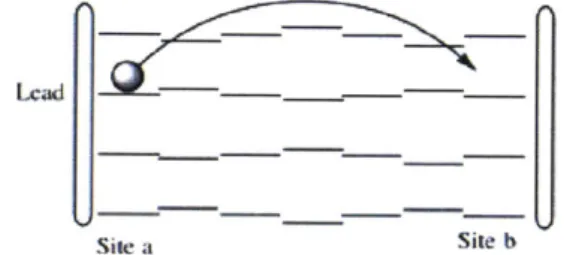
The graph below illustrated a transmission process [26, 27]:

Lcadb

Site a Site b

Figure

4.

disordered system.

Principally, in order to discover the transport properties of a system, the

first term needed is the transmission coefficient. The transmission coefficient

(also called the scattering matrix, S-matrix) tells the amplitude, density of

a particle to be at a different location from where it was. [31, 32]

|Outgoing) = S * Injected)

Thanks to the transmission coefficient, people can then easily access the

conductivity, delocalization length and so on.

The transmission probability T for a particle flying from site a to b can

then be expressed in terms of transmission probability [31, 411:

T

ISa,b21

where G is the green function. In mathematics, the Green function always

appears in the problems of inhomogeneous differential equations. Physically

speaking, the Green function here acts as a filter that distinguishes the values

that cause singularities. Moreover, the Green function can be considered as

a generalized transmission S-matrix.

O*R=S

R = 0-'S = G * S

where

0

Then we can simplify the problem to

(E

- Ho)<i

-

S

which results in

G = (E - Hop)-'

with Hp, being the system Hamiltonian of operator 0.[32] Hence for the Anderson Model, we shall have the following:

G = (H - E + i)-

where E is the energy variable, H represents the Anderson system and E is an imaginary number to avoid singularities that cause the system to collapse. The term of ic turns out to be exp(ic *m) in further calculations. In addition, c could be also thought of as a consequence of self energy, which will be discussed later in this chapter. [31]

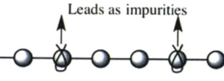
The system with impurities are sandwiched between two leads, from which particles with different energy E will be injected into the system. Leads itself can be viewed as a type of impurity in this larger tight binding system. Therefore, leads will also compel the system, which is called the 'self energy' E. [311 This self energy ultimately becomes the imaginary part of the Green function.

Leads as impuriti s

Figure 5. Self energy implied from leads as impurities.

2.3

Green function and Self Energy

Self energy [31,32,41] denotes the influence of the two leads onto the system, which will affect the behaviors of the sites close to the leads. If the self energy is large, leads tend to be two huge defects and the entire system will show few active signs. [3, 26]

The Hamiltonian of the Anderson Model only has been mentioned above and, hence, the corresponding Green function including self energy is the following :

G

where E screens through the continuous energy levels (variable) and E is the effect imposed from leads to the conductor.

Self energy E, is determined by right and left leads:

El=EL+ R

FI =

Gt G Gxc

Then for either side, the self energy is,

0

0

t

0

0

0

0

0

0

.0

0

H

0

0

0

0

0

0

t

0

0

0

- -0

with H being the Hamiltonian of a tight binding chain with nearest

neighbor coupling of unit 1 and 0 unit for on site energy.

The only existing element in Y would be the E(1, 1) and E(n, n) for a

lead containing n sites.

The symmetric tridiagonal matrix can be solved analytically.

cos[(n + 1)A]

-

cos[(n

-

1)A]

2sin(A) * sin[(n + 1)A]

where E + it = -2cos(A). [43]

Simplification of the equation above results in real and imaginary parts

that behave as in Fig. 6:

-2 - I 1 2

Rca)

Figure 6. Real and Imaginary part of self energy.

Explicit representation of the real and the imaginary parts can also be 0A OA-0.4 -2 -l0 1

0

derived [30, 31],

ReE

(r. -

-\/2n--

t

E

where V is the coupling constant between lead the conductor, t is the site coupling in between leads. The explicit representations act in the same way as those in Fig. 6.

If t >> E , but less than infinity, then the imaginary part can be treated

as a constant [32],

J~ny/4t2 _ 1 Im = -V2 V

t

Then for a particle to transmit from site a to b, its transmission proba-bility becomes easier to reach by having

T

=I(aIGIb)1

T

=

I

(a|Gc

b)

where |a) and 1b) are the vectors in position space, e.g the first site I

0

|1)=

0

0

0

0

0

In)=

0

[43].

and none of its eigenvalues is 0, A can be decomposed to A = VUV' and

A

=VU

V'.

2.4

Conductivity

Conductivity (g) is positively proportional to transmission probability at 0 degree Kelvin and can be directly calculated from the following equations [26, 321. In a 1-D Anderson Model, infinite long nearest neighbor coupling with impurities, conductivity is supposed to be zero, as all the states are localized. A general Landauer Formula reveals a new page in conductivity. Computation of Landauer Formula uses the form of Kubo equation [38, 391.

e2

g

=

(ITI)

= Tr(EG'EG)

7rh

where G is the Green function containing the lead effects and E is the self energy.

To derive the Landauer Formula above, a Fisher-Lee formula in GF rep-resentation is required [33, 37, 38].

Fisher-Lee formula in GF representation

To obtain the conductivity in this 1-D model, I need to calculate the

current

(j)

of this system first. Derived by Landauer and Buttker [35,

36,65-67], current in a finite system with possible disorders can be written as

ie

,= - (

pHicc

where d1, 4

c, are the wave functions of the left lead, conductor and the right lead. It is then necessary to study more in the system, as well the effects brought from both leads.

H, Hlc 0 #1 Ol

Hl'c He H'c

#c

=E

0

Hrc Hr

Or

(O

Solving the equations above, the following is obtained:

01

Or = GrHtcGself Hsbin

#c

with Gself being a full green function with self energy, Oin standing for incoming waves and Or for reflected waves from the left. [39, 40]

To calculate the current from lead to conductor, we will have [35, 34, 36]:

ie

jl =

(#IHic~c - #c Hi'c~)

#',H

Ic(G'

G,)HicGel H r'coin)

- e0 _{G'e 1 (H HlG'c}

~

=

_{($'nHicG'self E Gel Hs#in)}

h

As a result, we will have

|TI = 27r 6(E - E,)\)'fHicG'self

YGsclf Hs il)

= 27r

3

=

Z(

6(

6 6

= Tr(ErGself EiGself)

Consequently,

g(E) = Tr(EG'FG)

where E is the self energy and G is the Green function. This general equation sums up the probability of transmission for particles injected at different E. But since at 0 degree Kelvin, the only active energy level is the Fermi Level, the faster way can be used. [43]

3

Random Matrix Theory

3.1

Background

Random matrices are matrices with independently identically distributed (i.i.d) entries. The most common random entities obey the Gaussian dis-tribution. Random Matrix Theory (RMT) plays many roles in science for numerical analysis, mostly for stochastic problems. [44, 69, 68]

Random matrix theory was first introduced by Wigner in 1951 to statisti-cally study the resonances of neuron scattering in nuclei. [45-49] Since there were no good methods to calculate the energy levels other, Wigner thought that statistical understanding of the energy levels would be an alternative. Application of random matrix theory turns to be a huge success in measur-ing systems' mean eigenvalue spectrum and other properties for the use of further predictions.

Following Wigner, other scientists continued the study on random ma-trices, such as Dyson, Metha, Porter, Thomas and many others. [50-53, 55, 56, 58] The most famous one is Dyson. He crowned Random Matrix The-ory as a new type of statistics, because it is an accumulation of ensembles of different systems, rather than clustered results from identical systems or aver-aging through number theory. Random matrix theory minimizes the special characteristics of each individual system, which is also called the universal properties. [50, 51] Later on, Dyson explored further in random matrices and defined the following three situations. First, time reversal invariant with rotational symmetry, Dyson index 8 = 1; second, they are NOT invariant at time reversal symmetry (i.e charge carriers in external magnetic field), Dyson index 6 = 2; third, time reversal invariant plus half integer spin,

3

If random numbers in the Hamiltonians follow a Gaussian distribution, then they are Gaussian Ensemble, one of the most well studied matrix

en-sembles. The others are 1. Wishart

2. Manoca 3. Circular.

Gaussian Ensembles are divided into the Gaussian unitary ensemble (GUE), the Gaussian orthogonal ensemble (GOE) and the Gaussian symplectic en-semble (GSE). GUE are n * n unitary matrices with Gaussian distributed entries; GOE are n * n orthogonal ones and GSE are symplectic ones.

Given N = randn(n, n) with every numbers in the n * n matrix N having a Gaussian distribution,

GUE matrices are formed by (N + NH)/2; GOE matrices are formed by (N + NT)/2;

and GSE matrices are formed by (N + ND)/2, where ND is the dual transpose of the N. [44] The three types of Gaussian ensembles correspond to the three systems defined by Dyson. GOE stands for the system with time invariance and rotational symmetry; GUE stands for the system with complex numbers and not invariant under time reversal symmetry; GOE is for the rest.

Within these three ensembles, GUE/GUE are the most frequently used. An interesting and crucial property of these two ensembles are their eigen-value spectrums. [45] Wigner discovered that the distribution of eigenval-ues of GUE/GOE forms a semi-circle when the size of the matrix tends to be infinite.[46] The distribution can be exactly and analytically calculated through standard procedures. Starting with an arbitrary probability distri-bution function (p.d.f) for matrix entries, a good matrix factorization will be needed so that the derivative of the matrix can be then used to generate the joint density of the ensembles. For example, spectrum decomposition will be a good matrix factorization for GUE/GOE, applying the derivative of the

matrix [44]

for matrix GOE or GUE = QAQ'. We than can obtain the density by

summing over the eigenvectors. Therefore, the following is received:

1

lim p(dx) = p(dx) = 4 - x2dx

N-o 27

whose moments are

or, xk) Ck12 _{0 k=even}k=odd

where Cnis 30 25 20 - S15-0_ LL 10 5

0

the nth Catalan number, C= n=1 (2n). [60, 61]

Distribution of a random matrix

0

eigenvalues

In 1960, Dyson again named a new type of ensemble, the circular ensem-ble. Circular ensemble can be formed by exponentiating any one of these three ensembles with unitary matrices and then applying the Haar measure-ment (rotation invariance). [51] This new ensemble works no longer with Hamiltonian of a system, but indeed with the unitary scattering matrix for a scattering process. [62]

In mid-1990, as reviewed by C.W. Beenakker, Random Matrix theory has been applied into physics to solve many different questions, including S-Matrix modeling and so on. [63-781 However, those problems usually require diagonalization of tons of huge matrices and are, therefore, expensive. So is there any better and fast tool that people can use? One newly rise topic in Random Matrix Theory is free probability. [71-76] This is a very convenient tool to approximate the eigenvalue density from the two matrices that are partitioned from the original one.

3.2

Free probability

Free probability is a popular topic in the Random Matrix Theory due to its function as an algebraic structure for non-commutative matrices. [44, 601 It provides a fast way to approximate the distribution of eigenvalues for random matrices. Free probability view matrices differently from the classical probability, as it takes the eigenvalues of the sum of random matrices. [44, 78, 79] As the eigenvalues As of the sum of a series of Gaussian random matrices, it is not normal any more. And free probability shows that as the size of the matrix tends to be infinite, as well the number of samples, A will be a semi-circle distribution. In free probability, Wigner's semi-circle distribution law is similar to the normal distribution in the non-free theory. In addition, free cumulants take the place of regular cumulants, as free cumulants are simply non-crossing partitions of a finite set, rather than all partitions for those regular cumulant. [80, 74, 75]

Within free probability, one key term is free convolution. People can split a single matrix into two easier matrices and find the distribution of eigenvalues through free convolution. It is always a pity that, regularly, the eigenvalues of the sum of two matrices is not the sum of the eigenvalues of each matrix

for non-commuting A and B), since the contributions from eigenvectors are neglected. [44, 81] While in some cases, the distribution of the eigenvalues of the Haar measured matrix tends to be additive free convolution for that of two random matrices separated from the origin one. [81] (Haar measured matrix - invariant of base, freely independent matrices). [47]

3.2.1

Free convolution and Free Rotation

Convolution can tell the probability distribution function (p.d.f) of the third function that is composed of two known functions. Free convolution involves randomness within probability measures. [46]

Let us denote PA to be the distribution of matrix A and pB to be that of matrix B. Free convolution A E B is defined as

1

RAEBB(w)= RA(w)

+

-where R is the R - Transformation of px[82, 83].

W= lim P p(z) dz

E

_{f Rx1(w) - (z + i.)}

R

with some R-transform can be obtained through expansion of power se-ries:

GA(w) = iimf ( .dz

=

R k=O

where Pk is the kth moment of px.

cc

RA(w)= _RA(W)

SVk

Wk+l k=O

and Vk are the free cumulants, which is the combination of moments and

Vk(A

E

Q

on B, A

+

QBQ',

has the same p.d.f of the A ED B as the size of the

matrix becomes infinite. Here

Q

is a unitary random matrix generated by

QR decomposition of a fully random matrix N. [82]

p(Eig(A + B)) ~ p(Eig(A + QBQ'))

3.2.2 Free convolution applied to the approximate of density of state

Previously, research has been done to approximate the density of state

(equivalent to the p.d.f of eigenvalues) in the Anderson Model, mimicking

the non-crystal organic materials. It proves that free convolution did a great

job that the error for the approximation can be as small as the 8th moment.

[82, ??]

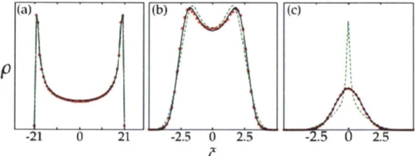
Figure 7 shows how free convolution works as nearly a perfect

approxi-mation to the traditional calculation.

(a) (b) \ (c)

-21 0 21 -2.5 0 2.5 -2.5 0 2.5

Figure 7. Cropped from [81j, Density of States, obtained from 5000

sam-ples pool of 2000 by 2000 matrices with small (a), medium (b), large disorder

(c) (disorder Z=0.1, 1 and 1); Red: exact diagonalization, Black: Free

con-volution with partition of diagonal+tridiagonal, Green: Free concon-volution with

partition of upper left tridiagonal and bottom right tridiagonal.

Errors for the approximation can be calculated from:

w() WI ') + k - ()kW(k) + OwI(k+1))

where w is the p.d.f of eigenvalues from regular calculation

infd

(r) = exp(Z (

n"

n=1

W' is the p.d.f of eigenvalues form free approximation, Pk is the kth moment, and rn is the finite cumulant.

The k"h moment

Ilk =((A

+

in which j> m1

+ nj = n

((AB)

--

(g

n

with gi being the diagonal random entries. With the partition of

1 0 0 0 c 0

0 '-. 0

+

0 0 3 ) 0 C 0

error can be minimized to the 8th moment, E = 2a-4J4/8!.

In general, 1-D nearest neighbor model has an error of (AB)4 = 4;r 2-D square has an error of (AB)4 - j4;4

Another partition is also tested:

g1 C 0 '.0 0

A2+ B2= c 0 0

+

0 g, c

0 0 *.. 0 C 0

However, the approximation does not behave as perfect as the previous par-tition method, due to a difference of -₄ for its fourth moment which does not appear until the eighth in the previous partition method.

(A2 +B2) 5(A EBB2 2)

and

(A2B2) = (J2 +

0.

instead of (J2 + 12)2

.[85]

3.3

RMT supported (Artificial) Neural Network

A recent study by Karoui, shows that analytical decompostion of a system with randomness can be less productive. Instead, people should probably switch their way of thinking to a more 'fruitful' statistical optimization re-lated solution. [86]

(Artificial) Neural Network (NNT) will be introduced here to find the eigenvalues and the corresponding eigenvectors for largely disordered system that cannot neither be approximated using perturbation theory or can only use conventional decomposition methods. Traditional decompositions usually involve transformations with high time complexity, around O(n3_{) and}

some-times even O(n!) or O(n'). Even after improvement, such as the formation of a Hessenberg matrix first, those decompositions still take at least knr3_+0(n2₎

time complexity. [18] Well designed NNT architecture, i.e Architecture I and II below, can not only turn matrix multiplication into matrix-vector multi-plications but also parallel optimize all eigenvalues and eigenvectors at the

same time. Hence, there will be a huge reduction in computation time.

(Artificial) Neural Networks were inspired by biological neural nets in

brains. Many studies have been done on the applications of neural network to

spectrum decomposition. However, most of them are solving the maximum,

minimum or a certain eigenpair. [95, 96] None of them were trying to provide

methods that can enhance the speed by offering more accurate initial guesses.

Neural Network is a great choice since a good architecture can well split

the calculations into highly efficient parallel computations and avoid matrix

multiplications. A group of scientists succeeded in applying neural networks

to signal processing and other engineering computation problem. [97, 98j

How-ever, their architectures are still not perfect and need to be tailored so that

it will fit my matrices the best. The following two architectures have been

built after modification of Cichocki's network.

x

SJIAI

X

II

4a

x

x

x

I

Architecture I can be considered as a time-series neural network. The original matrix that produces only real eigenvalues, A, forms its two hidden layers. To-be-adjusted inputs include pairs of eigenvalues and eigenvectors, which will circulate in the system and pass through hidden layers until opti-mization is done. Architecture I is designed to calculate eigenvalues, as well as their corresponding eigenvectors, within a known range. This architec-ture is fast, as jobs for each pair of eigenvalues and vectors can ideally be assigned to n or more cores. In other words, the time of calculating n pairs of eigenvalues and their eigenvectors is the same as that of one pair, given enough cores are available. With current amazing development of hardware, the requirement above is not hard to realize. Nevertheless, Architecture I also shows that only one optimization is needed, which again reduces the time complexity. [97]

Architecture I decomposes matrices by solving a set of nonlinear algebra:

(A

-

Ail)vi

=

0

for i = 1, 2, 3... n.

Here the eigenvectors vi must be orthogonal and hence vTv = 1 becomes part of the constrains.

Once initial guesses for each pair of eigenvalues and eigenvectors pass through the first layer, self error will be collected and calculated by

Zaij

-1=1

Aivli. Immediately after that, self error will be combined with new errors

from guesses passing through the second layer. As long as guessed values are non-trivial, system will function properly.

Optimization is measured by the following cost (performance) function:

Err(vi, Ai) = 0.51ekI2 + _(En ₁ v - 1)2, where el is the self error.

and eigenvectors are

dAj

dErr

jd=it

dA

Z

elvii

and

dvjnn

=

-p(Zeaj

-

Aje

+ rnvi(Zv'

-

1))

1=1 1=1

forj

1, 2, 3...n. a and

#

_{are the learning rate and the penalty constant.}

Increasing a can decrease the computation time, since 6vi and 6Aj become

larger. However, system can diverge or break by reaching the computation

#

com-putation time, as the cost function is in positive proportion to ,. However,

large

#

_{can improve the calculation speed when the initial guess are too far}

away from the real eigenvalues.

3.3.2

Architecture II

X(0t V, W V C

V 0

2

V and the eigenvalue matrix, W. Architecture II can simultaneously find

all eigenvectors and eigenvalues. A list of independent orthogonal (training) samples or excitation vectors x are injected into the system, going through hidden layers, followed by eigenvector matrix V and eigenvalue matrix W. The outputs will continue into two tunnels after another layer of V. One will react with Ax to verify the accuracy of both W and V. The other one will react with V to check the orthogonality of the eigenvector matrix. The entire process won't stop until the cost function meets the minimum requirement. Optimization speed can be easily and largely enhanced by setting large learning rate. Accuracy is controllable. Here the cost function is set to meet the max value of 10', providing no more than two sig. fig difference in the final approximation.

Architecture II employs A = V * W * V-1, where the eigenvector matrix V has to be orthogonal again, V *

V'

V'*

I.

Two types of error, el and e2, form the major part of the cost function,

1

+

je

I2

Ax

r

and T is the penalty constant.

steepest decent'method:

dvi

dt

6%

s

dAi

dt

A

for i - 1, 2, 3... n.^/ andY_{2 are the two learning rates for each tunnel,} respectively.

After simplification, the following equations can be derived:

n

dvi

'71(eii

cit

1=1

cit

Again, convergence can be manipulated by adjusting the learning rates and the penalty constant, /1 , -y2 and r.

The calculation speed of Architecture II can be improved by having some fun excitators. Excitator x(t)s have been replaced by identity matrix of size

n, rather than random orthogonal vectors,

[Sin(wt),

In this case, calculations of weights turn out to be much easier and faster, as matrix multiplications become additions or simply a certain column of itself. For instance, V * x(t) = V(:, t). However, after multiple tests, a memory

related problem accumulates as the size of matrix gets larger. Hence, timing becomes inaccurate. As a result, Arch II can be a future project.

3.4

Topping neural networks with Random Matrix

The-ory (RMT-RNN)

Like most of the other optimization processes, if the initial guesses are closer to the true values, it will take many fewer steps and therefore time to reach the thresholds. For both architectures, in order to even shorten computa-tion time more, RMT has been used to generate much more reliable initial guesses than random guesses. Since the Anderson matrices have proved to be partially free up to its 8th moment, it is proper to apply RMT here.

181]

RMT estimates the distribution of eigenvalues, based on which a list of initial guesses will be pseudo-generated and passed through into the system. However, in Arch I, the same initial guess might give different final optimiza-tion soluoptimiza-tions. That is due to random initial guessed eigenvectors.

3.4.1 Eigenvector stabilization

Fixed -A algorithm has then been created to stabilize eigenvectors. The main idea is to find

Argmine|Av - AfiedVl.

Put random eigenvectors vi for guessed Ai into the first step of Arch I. During this step, JA is set to be 0. Before the regular Arch I runs, stabi-lized eigenvector Vi,stable will take the place of vi. Total time of calculation increases, but still lower than the traditional decomposition. Meanwhile, less time has been spent on the optimization steps, as right now, both eigenvalues and eigenvectors are closer to the true values.

3.4.2 Radar Algorithm

Rather than stabilizing eigenvectors, it is also a good idea to screen out all eigenvalues near a few guessed points using various random eigenvectors. This method is similar to the excitation inputs of Arch II, with v(k) being

the excitators.

sin(i)

Vinitial guess(k)

sin(2i)

[

sin(ni)

In this way, true eigenvalues near the initial guesses can all be found by

pumping random eigenvectors into the system.

4

Methods

Taking advantage of free probability, I separated the Hamiltonian of Ander-son Model, H., into two parts, one matrix with only the site coupling and one with disorder that was free-rotated later on.

Hc - HO + Hmpurity

4.1

Transmission probability calculation during the

ear-lier period of research

At the beginning of this research, focus was on how free addition will affect transmission probability. Eigenvectors are controlled so that they are away from free rotations. Additionally, the model is based on particle in a ring (PIR), a simple version of the Anderson Model, and, hence, no influence from the leads is included.

For particle in a ring model(PIR), transmission probability can be ob-tained by an analogy between PIR and an infinitely long chain

T = j(+k

|GI

+ k)|

for a particle starting at site 0 with state function

I+k)

n.

The wave functions and energy for each level k can be written as

exp( 2,Tki)

exp(2 2)rki

I+k)

exp(3

_LrL)

exp(n2 'ki)

and E(k) Jcos(2 k), respectively. [23]

In larger system, we will be able to get more accurate simulation due to smaller bias of Gaussian Distribution. Green function, G, here acts as a filter that only allows wave at a certain energy level k to go out, G=

_~H-IE(k)

IGI

and the transmission probability is simply just its square, 1(+k

IG

Results can be random and full of noise due to two problems: 1. errors occur during random selection of the Gaussian numbers; 2. these random numbers changes the states of 'free' particles. Therefore, external energies, mean(diag(gi)), are added from each site to reduce the bias. Our matrix turned out to be: Ho + Himp tr(V) _n + xJ. Since free probability will lead the

eigenvalues of H ~ Ho + QHimpQt, then what would happen if we turn the basis of impurity Himp freely, would that change the transmission coefficient? For simulation with free rotations, a unitary matrix

Q

Calculations of the transmission probability were run many times, with 1000 runs as a standard. All data are then collected, histogramed and plot-ted.

4.2

Conductivity

More factors, such as self energy, appear in the following equations to receive the total conductivity of a more completed Anderson Model. The following shows how free approximation are computationally applied to conductivity.

Similar to the thinking flow in 4.1, the corresponding Green function were converted into two parts, with noise being free rotated:

G/--I Q H - E - EI

=(HO - E - EI) + Q' * Hemnp * Q

1 0 0 0

1

E

0

0

0

+ Q'*

1

where E is the energy of particles injected into the system, E is the self energy and

Q

Here again, to make everything more convenient, constant of the site coupling has been normalized to 1.

Now, I replace the G in T = 2Tr(EG'EG) with G' as the result of free

approximation.

conductance for a 1-D Anderson model. For each run, the unitary matrices

Q are created from a new Gaussian random Hermitian matrix. Results were collected and then histograms were made. Variables are controlled as the following: screening through different sizes of noise N(0, '), different length of the chain n, different positions of impurities, different injected energy E, etc.

The size of noise is denoted as ", where o- is the standard deviation of Gaussian distribution and J is the coupling constant. The size of the matrix, also called the length of the chain in a 1-D chain model, could be easily adjusted. In addition to the trial free rotations of diagonal Hmp, matrices with only site coupling was also freely rotated while keeping Himp fixed. Despite that, impurities were added not only onto on-site partitions, but also onto off-site partitions (tridiagonal lanes) for systems with more than site defects. Values of E were screened from 0 unit to 5 unit with increment of 0.1 unit, as E ranges from 0 to 2J in a pure system. E were set to be 1 * i

Recall that

v2

E

FE

EY,

(

i 1-()2)

t 2t 2

in which t is the coupling constant between the lead and the system, V is the density of state (DOS) at energy E. When t is large enough, the imaginary part becomes -i 2 . If V is close to zero, then the imaginary

part will disappear and physically there won't be enough number of particles to go through this test. Hence, V needs to be large enough to propagate adequate particle samples for the test. After a couple of tests, 1i turns out to be the best value for E. One other effect of E, is that larger self energy will influence almost every site and curve the conductivity too much, while smaller self energy leads to peaks that are too sharp.

sample pool by following the algorithm below.

Program Algorithm to calculate conductivity

1. Produce an n by n matrix with every diagonal terms to be Gaussian distributed N - (0, o-) and tridiagonal terms to be 1;

2. Partition the matrix into desired structures;

3. Generate a random real matrix N whose entries follows Gaussian again;

4. QR decompose matrix N and receive the orthogonal matrix

Q;

5. Apply

Q

X is the part selected;

6. Calculate the Green function approximate G' = (H' - EI

+

7. Obtain the Transmission Coefficient by the formula T

I

(a

IG'I

b)

9. Repeat steps 1-8 for 10000 times; 10. Collect data for conductivity; 11. Histogram the data and plot.

4.3

RMT-RNN

All codes of RMT-RNN and baseline QR algorithm are in MATLAB level language. Other than basic matrix operations and conditional functions, such as 'for', 'if', 'while', no built-in functions are directly called. Hence, built-in commands using a second or third languages are avoided, which maximizes the fairness. QR algorithm came from the textbook written by 0. Routh and was fully tested with numerous matrices. [18]

4.3.1

Architecture I (Arch I)

For Architecture I, since it is a time-series neural network, no external injec-tions are necessary. Arch I will not generate results until the cost function is minimized to a designed threshold. Since, by default, MATLAB provides 4 digits after decimal point, thresholds of 106 are chosen, indicating errors less than 0.000001. Convergence properties of RMT-RNN, the speed test between RMT-RNN and the QR algorithm are tested under different values of penalty, learning rates, r and p and with or without an eigenvector sta-bilization algorithm. Matrices applied are not only the Green functions of the Anderson model, but also random symmetric matrices and matrices that were normally used in related papers. For each control, 2000 runs are con-ducted and results are collected. Due to limit of computation power, only matrices with size up to 100 have been fully tested, with RMT becoming effective for n > 50. Fewer runs were performed on matrices with size from 100 to 1000. The purpose of larger matrices is to show the continuity of Arch

I.

4.3.2 Generating guesses of eigenvalues

Both Anderson random matrices and regular Hermitian matrices were tested. For Anderson matrices, form the distribution of eigenvalues by either analyt-ically calculating the distribution from RAW1B = RA + RB - I or accumulating

the eigenvalues of A + QBQ' . For regular Hermitian matrices, their eigen-value distribution follows tthe Wigner semi-circle or can be computationally generated and collected.

Next, pseudo-guesses initial values from the distribution formed above. Dump the initial guesses into Arch I.

Pseudo-guesses can be formed by the following Algorithm:

distribu-xq=-[min(t): (max(t)-min(t))/n:max(t)];

pdf=interp1 (t,h,xq,'spline') % find p.d.f of the distribution using samples-step 1;

pdf=pdf/sum(pdf);

cdf=cumsum(pdf)% if analytically find the distribution via RA EB RB or concrete p.d.f is known already, start here;

[cdf,mask] =unique(cdf)% get rid of cdf with same values;

rv=rand(1,1.5*n) % randomly select 1.5*n number of pseudo samples to avoid possible missing values. Empirically, 1.2 is enough, coming with a missing rate of 0.2% over a test of 1000 runs

proj=interpl(cdf,xq,rv); % inverse step 1; find the samples based on c.d.f; proj=proj+0.0001; %avoid psudo-number of zero values.

4.3.3 Eigenvector stabilization

Set 6A = 0 and only allow changes in eigenvectors. For each initial guess, Arch I with fixed 6A should generate the eigenvector corresponding to the guessed eigenvalue.

4.3.4 Radar Algorithm

Based on the distribution of eigenvalues, round(n/l) points are chosen, where I is the number of intervals you want to set. For each point,

sin(i) sin(2i) sin(x) sin(3i)

will be injected into Arch I as the initial guess for eigenvectors for i = [1,

1].

5

Results and Conclusions

5.1

Transmission probability during earlier period

Transmission probability is framed on the model of particle in a ring (PIR).

Neither free rotation of the eigenvectors nor the self-energy from the leads

are included in the model yet (there is no leads).

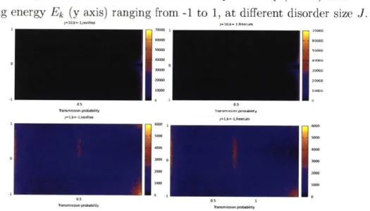
The graph below shows the transmission probability (x axis) after

screen-ing energy

_{(y axis) ranging from -1 to 1, at different disorder size J.}

jl10.=1, II*0I10,k--I.freooc.. 1 o 70000 0000 60000 60000 50000 S0000 30000 :0000 20M0 20000 100001W0 e

'ansmIso pliabilission T-o4- V rgsht s i cc ,kn-c,nontrom let),k1-f.eott ud 0 3000 3M% 2000 ₂₀₀₀ low0 ₁₀₀₀ 0.5 0 . 05 1

lrisiso probablity -R ns Wsww pobwbxw~

Figure 8. Transmission probability V.S energy shift on sites. J=10, origi-nal calculation (Top left); J=10,

free

free

Fig. 8 tells that transmission probability has a tendency towards 1 for

large coupling J (J=10) at all other energy levels, except for the resonance

state (x = 0). Because particles can easily transmit within the 'band' formed

by the coupling, transmission can more frequently occur than reflection. On

the other hand, for smaller J (J=1), transmission coefficients tend to be 0

with some to be 0.5, as charges are scattered and localized by relatively

large impurities. As in a 1D real system with frozen disorders, transmission

coefficient could tell us the trends for waves to be reflected by disorders.

Free rotation plays as good role as the original calculation. Calculations

with free rotation show similar patterns to those of the original calculation.

As to how accurate the approximation is, we will run a further error analysis.

5.2

Transmission probability and Conductivity

Approx-imation using Free Addition

Following the instruction in the method chapter, I received the data below:

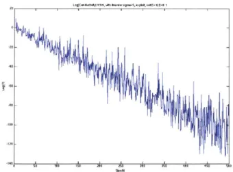
To validate the initial conductivity formula, I tested the transmission

coefficient (squared) along the length of the chain with disorder o-

=

5, Self

energy E

1

* i and fixed the energy level at 0.1 unit. According to the

conjecture, the transmission coefficient should exponentially decay as the

length increase. Therefore, I took the logarithm values and a line came up.

Due to the capacity of the computation, deviation increased as the value of

transmission coefficient got close to zero at a long chain.

-20A1..

Figure 9. Log(Conductivity) Versus Size N of Matrix. The line proves the exponential decay of conductivity as the size of the matrix is increasing.

I

11!'t ~

-140 A i. A- -i. =I. i =h i. i