Alcohol and Self-Control: A Field Experiment in India
The MIT Faculty has made this article openly available.
Please share
how this access benefits you. Your story matters.
Citation
Schilbach, Frank et al. "Alcohol and Self-Control: A Field
Experiment in India." American Economic Association 109, 4 (April
2019): 1290-1322 © 2019 American Economic Association
As Published
http://dx.doi.org/10.1257/aer.20170458
Publisher
American Economic Association
Version
Final published version
Citable link
https://hdl.handle.net/1721.1/126690
Terms of Use
Article is made available in accordance with the publisher's
policy and may be subject to US copyright law. Please refer to the
publisher's site for terms of use.
1290
Alcohol and Self-Control: A Field Experiment in India
†By Frank Schilbach *
This paper studies alcohol consumption among low-income work-ers in India. In a 3-week field experiment, the majority of 229 cycle-rickshaw drivers were willing to forgo substantial monetary payments in order to set incentives for themselves to remain sober, thus exhibiting demand for commitment to sobriety. Randomly receiving sobriety incentives significantly reduced daytime drink-ing while leavdrink-ing overall drinkdrink-ing unchanged. I find no evidence of higher daytime sobriety significantly changing labor supply, produc-tivity, or earnings. In contrast, increasing sobriety raised savings by 50 percent, an effect that does not appear to be solely explained by changes in income net of alcohol expenditures. (JEL C93, D14, I12,
J22, J24, J31, O12)
Heavy alcohol consumption among male low-income workers is common in India and other developing countries. Excessive drinking can have severe consequences for individuals and their families, yet our understanding of such effects is limited. In particular, acute alcohol intoxication is thought to affect myopia and self-control, such that alcohol consumption could interfere with a variety of forward-looking decisions and behaviors. By affecting productivity, labor supply, savings decisions, and human capital investments, alcohol could reduce earnings and wealth accu-mulation and thus deepen poverty. However, though theoretically possible, we do not know whether such effects are present or economically meaningful in reality.
* Department of Economics, MIT, The Morris and Sophie Chang Building, 50 Memorial Drive, E52-560, Cambridge, MA 02142, and NBER (email: [email protected]). This paper was accepted to the AER under the guidance of Stefano DellaVigna, Coeditor. I am deeply grateful to Esther Duflo, Michael Kremer, David Laibson, and especially Sendhil Mullainathan for their encouragement and support over the course of this project. I thank the editor for his excellent guidance and three anonymous referees for their helpful comments. I also thank Nava Ashraf, Liang Bai, Abhijit Banerjee, Raissa Fabregas, Edward Glaeser, Simon Jäger, Seema Jayachandran, Larry Katz, Aprajit Mahajan, Nathan Nunn, Matthew Rabin, Gautam Rao, Benjamin Schöfer, Heather Schofield, Josh Schwartzstein, Jann Spiess, Dmitry Taubinsky, Uyanga Turmunkh, Andrew Weiss, and participants at numer-ous seminars and lunches for helpful discussions and feedback, and Dr. Ravichandran for providing medical exper-tise. Kate Sturla, Luke Ravenscroft, Manasa Reddy, Andrew Locke, Nick Swanson, Louise Paul-Delvaux, Sam Solomon, Simon Schröder, Zhili Liu, and the research staff in Chennai performed outstanding research assistance. Special thanks to Emily Gallagher for all of her excellent help with revising the draft. The field experiment would not have been possible without the invaluable support of and collaboration with IFMR, and especially Sharon Buteau. All errors are my own. Funding for this project was generously provided by the Weiss Family Fund for Research in Development Economics, the Lab for Economic Applications and Policy, the Warburg Funds, the Inequality and Social Policy Program, the Pershing Square Venture Fund for Research on the Foundations of Human Behavior, and an anonymous donor. The study was approved by Harvard IRB (CUHS protocol F22612). The author declares that he has no relevant or material financial interests related to the research described in this paper.
† Go to https://doi.org/10.1257/aer.20170458 to visit the article page for additional materials and author disclosure statement.
Moreover, little knowledge exists about policy options to alleviate the potential neg-ative impacts of alcohol.
Since alcohol consumption has long been associated with self-control prob-lems, commitment devices could help improve outcomes. A hallmark prediction of economic models of sophisticated agents with self-control problems is demand for commitment devices which allow individuals to curb their future self-control problems by increasing the relative price of undesirable choices. Previous papers have considered the impact of commitment devices in a number of domains, includ-ing savinclud-ing, smokinclud-ing, and intertemporal effort provision. Existinclud-ing evidence shows that the availability of commitment devices does indeed help, at least in some of the cases (Ashraf, Karlan, and Yin 2006; Kaur, Kremer, and Mullainathan 2015). However, few real-world examples of successful commitment devices exist, and empirical evidence of positive willingness to pay for such devices is scarce, call-ing into question the underlycall-ing models and the efficacy of commitment devices (Laibson 2015, 2018).
Against this background, this paper considers alcohol consumption among cycle-rickshaw drivers in Chennai, India, a population for whom drinking is likely a serious problem. In a 3-week field experiment with 229 men, I offered finan-cial incentives for sobriety to a random subset of individuals, while a second group received unconditional payments of similar magnitude. The remaining individuals were offered the choice between sobriety incentives and unconditional payments. The randomized nature of the experiment allows me to investigate the impact of increased sobriety on labor market outcomes and savings behavior. To measure the impact of acute intoxication on intertemporal choices, all subjects were provided with a high-return savings opportunity. For a cross-randomized subset of study par-ticipants, the savings account was a commitment savings account, i.e., individuals could not withdraw their savings until the end of their participation in the study.
Individuals’ choices between sobriety incentives and unconditional payments reveal substantial willingness to pay and thus demand for commitment to increase their sobriety. In three sets of weekly decisions that each elicited preferences for sobriety incentives in the subsequent week, over one-half of the study participants chose the incentives when they were weakly dominated by the unconditional pay-ment option. Even more striking, over one-third of study participants preferred incentives for sobriety over unconditional payments, even when the unconditional payments were strictly higher than the maximum possible amount that subjects could earn with the sobriety incentives. These men were willing to sacrifice study payments of about 10 percent of daily income even in the best-case scenario of vis-iting the study office sober every day.
This finding provides clear evidence for a desire for sobriety by making future drinking more costly, in contrast to the predictions of the Becker and Murphy (1988) rational addiction model, but in line with Gruber and K˝oszegi (2001). The observed demand for commitment indicates a greater awareness of and willingness to over-come self-control problems than found in most other settings, such as smoking, exercising, saving, and real-effort choices (Giné, Karlan, and Zinman 2010; Royer, Stehr, and Sydnor 2015; Ashraf, Karlan, and Yin 2006; Augenblick, Niederle, and Sprenger 2015). Since demand for commitment implies sophistication regarding an underlying self-control problem, the evidence also contrasts with recent evidence
documenting near-complete naïveté regarding present bias (Augenblick and Rabin forthcoming).
The financial incentives significantly increased individuals’ sobriety during their daily study office visits. Sobriety incentives decreased daytime drinking as mea-sured by a 33 percent (or 13 percentage point) increase in the fraction of individuals who visited the study office sober and equivalent reductions in breathalyzer scores and self-reported drinking. However, overall alcohol consumption and expenditures remained nearly unchanged. This finding implies that individuals largely shifted their drinking to later times of the day rather than reducing their overall drink-ing as a response to the incentives. In contrast to existdrink-ing evidence of persistent impacts of short-run incentives for health-related behaviors (Prendergast et al. 2006, Dupas 2014), financial incentives do not appear to be effective at persistently reduc-ing drinkreduc-ing in this context.
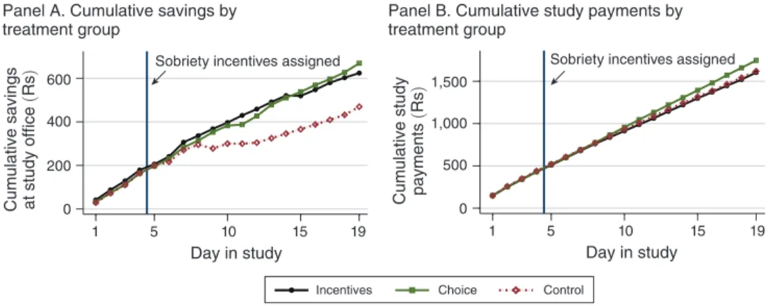
The increase in daytime sobriety due to the incentives provides a “first stage” to estimate the impact of sobriety on labor market outcomes and savings behavior. Perhaps surprisingly, I do not find evidence of significant changes in labor supply, productivity, or earnings, though I cannot reject treatment effects of about 10 to 15 percent for these outcomes. In contrast, offering sobriety incentives increased individuals’ daily savings at the study office by over 50 percent compared to a con-trol group that received similar average study payments independent of their alcohol consumption. Two potential channels contribute to this increase in savings: changes in income net of alcohol expenditures and changes in decision making for given net income. Given the lack of significant changes in earnings and alcohol expenditures, the sobriety incentives increased net incomes only slightly. It therefore appears that increased sobriety altered individuals’ savings behavior for given net income.
The relationship between the effects of sobriety incentives and commitment sav-ings provides further evidence of this hypothesis. I find that sobriety incentives and the commitment savings feature were substitutes in terms of their effect on savings. While commitment savings and sobriety incentives each individually increased sub-jects’ savings, there was no additional effect of the savings commitment feature on savings by individuals who were offered sobriety incentives, and vice versa. This finding suggests that alcohol causes self-control problems, in line with psychology research on “alcohol myopia.” Steele and Josephs (1990) argue that alcohol has par-ticularly strong effects in situations of “inhibition conflict,” i.e., with two competing motivations, one of which is simple, present, or salient, while the other is compli-cated, in the future, or remote. One interpretation of this theory is that alcohol causes present bias. The findings from my field experiment support this interpretation in the context of savings decisions and demonstrate that alcohol-induced myopia can have economically meaningful consequences.1
1 While there is considerable evidence that alcohol myopia affects a range of social behaviors such as aggres-sion and altruism, studies on alcohol myopia did not consider savings deciaggres-sions or intertemporal choice (Giancola et al. 2010). However, many cross-sectional studies, including several on alcohol, found a correlation between impulsive “delayed reward discounting” (DRD) and addictive behavior, without establishing existence or direction of causality (MacKillopp et al. 2011). Experimental lab studies consistently found acute alcohol intoxication reduc-ing inhibitory control in computer tasks (Perry and Carroll 2008), but studies on the effects of alcohol on impulsive DRD found mixed evidence (Richards et al. 1999; Ortner, MacDonald, and Olmstead 2003). My study differs from previous experimental studies in a number of ways. In particular, (i) the duration of the experiment was significantly longer (over three weeks versus one day), (ii) sample characteristics were markedly different, (iii) stakes were
This paper contributes to the growing literature on saving decisions among the poor. Several recent studies emphasize the importance of technologies for committing to savings and show that the availability and design of savings accounts are import-ant determinimport-ants of savings behavior among the poor (Dupas and Robinson 2013; Karlan, Ratan, and Zinman 2014). This paper shows that helping individuals to overcome underlying self-control problems regarding specific goods can be a sub-stitute for commitment devices for overall consumption-saving decisions. Finally, the paper suggests second-best policies aimed at reducing the costs of inebriation by shifting critical decisions away from drinking times could be welfare-improving even if they do not change overall drinking levels.
The remainder of this paper is organized as follows. Section I provides an overview of the study background, including alcohol consumption patterns in Chennai and in developing countries more generally. Section II describes the experimental design, characterizes the study sample, and discusses randomization checks. Section III considers the extent to which self-control problems contribute to the demand for alcohol by investigating rickshaw drivers’ demand for incen-tives. Section IV then describes the impact of increased sobriety on savings, and Section V investigates the interaction between sobriety and commitment savings. Section VI concludes.
I. Alcohol in Chennai, India, and Developing Countries
There is scarce information regarding drinking patterns in developing countries, especially among the poor. As a first step toward a systematic understanding of the prevalence of drinking among male manual laborers in developing countries, I conducted a short survey with 1,227 men from 10 low-income professions in Chennai in August and September 2014. Surveyors approached individuals from these groups during regular work hours and offered them a small compensation for answering a short questionnaire about their alcohol consumption, including a breathalyzer test. According to these surveys, the overall prevalence of alcohol consumption among low-income men is high (upper panel of online Appendix Figure A.1);2 76.1 percent of individuals reported drinking alcohol on the
pre-vious day, ranging across professions from 37 percent (porters) to as high as 98 percent (sewage workers).
On days when individuals consume alcohol, they drink considerable quantities of alcohol (lower panel of online Appendix Figure A.1). Conditional on drink-ing alcohol on the previous day, men of the different professions reported drinkdrink-ing
higher (relative to income), and (iv) the main outcome was the amount saved after three weeks. In the perhaps most closely related field study, Ben-David and Bos (2017) provide complementary evidence on the impact of alcohol availability on credit-market behavior using variation in liquor store opening hours in Sweden.
2 The prevalence of alcohol consumption among women in Chennai and in India overall is substantially lower. It is consistently estimated to be below 5 percent in India, with higher estimates for North-Eastern states and lower estimates for Tamil Nadu (where Chennai is located) and other South Indian states (Benegal 2005). In the most recent National Family Health Survey (Round 3 2005/6), the (reported) prevalence of female alcohol consumption was 2.2 percent (IIPS and Macro International 2008). It is highest in the lowest wealth (6.2 percent) and education (4.3 percent) quintiles.
average amounts ranging from 3.8 to 6.5 standard drinks on the same day.3 Since
alcohol is an expensive good, the resulting income shares spent on alcohol are enormous (upper panel of online Appendix Figure A.2). On average, individuals reported spending between 9.2 and 43.0 percent of their daily incomes of Rs 300 ($5) to Rs 500 ($8) on alcohol. These numbers are particularly remarkable since many low-income men in Chennai are the sole income earners of their families. Finally, 25.2 percent of individuals were inebriated or drunk during these surveys, which all took place during the day and during many of the individuals’ regular work hours (lower panel of online Appendix Figure A.2).
The substantial level of alcohol consumption found among male low-income workers in Chennai raises the question of how these numbers compare to other estimates for Chennai, for India, and for developing countries overall. Limited data availability of alcohol consumption and especially breathalyzer scores, as well as data inconsistencies make answering this question difficult (Gupta et al. 2003). However, there is reason to believe that the estimates for Chennai are not unusual compared to other parts of India or other developing countries. The WHO Global Status Report on Alcohol and Health provides country-by-country estimates of alco-hol prevalence and consumption levels (WHO 2014). According to this report, male drinkers in India, about one-quarter of the total male population, drink about 5 stan-dard drinks per day on average, only slightly less than the average of the physical quantities shown in online Appendix Figure A.1.
II. Experimental Design and Balance Checks
The experiment took place between April and September 2014. Two hundred twenty-nine cycle-rickshaw drivers working in central Chennai were asked to visit a nearby study office every day for three weeks each. During these daily visits, indi-viduals completed a breathalyzer test and a short survey on labor supply, earnings, and expenditure patterns of the previous day, and alcohol consumption both on the previous day and on the current day before coming to the study office. To study the impact of increased sobriety on savings behavior, all subjects were given the oppor-tunity to save money at the study office.
Participants were randomly assigned to various treatment groups with the following considerations. First, to create exogenous variation in sobriety, a randomly-selected subsample of study participants was offered financial incentives to visit the study office sober, while the remaining individuals were paid for coming to the study office regardless of their alcohol consumption. Second, to measure individuals’ demand for sobriety incentives and thus to identify self-control problems regarding alcohol, a randomly-selected subset of individuals was given the choice between incentives for sobriety and unconditional payments. Third, to examine the interaction between sobriety incentives and commitment savings, a cross-randomized subset of individ-uals was provided with a commitment savings account, i.e., a savings account that
3 I follow the US definition of a standard drink as described in WHO (2001). According to this definition, a standard drink contains 14 grams of pure ethanol. A small bottle of beer (330 ml at 5 percent alcohol), a glass of wine (140 ml at 12 percent alcohol), or a shot of hard liquor (40 ml at 40 percent alcohol) each contains about one standard drink.
did not allow them to withdraw their savings until the end of their participation in the study.
A. Recruitment and Screening
The study population consisted of male cycle-rickshaw drivers aged 25 to 60 in Chennai, India.4 Individuals enrolled in the study went through a three-stage
recruit-ment and screening process. Due to capacity constraints, enrollrecruit-ment was conducted on a rolling basis such that there were typically between 30 and 60 participants enrolled in the study at any given point in time.
Field Recruitment and Screening.—Field surveyors approached potential partic-ipants near the study office during work hours and asked interested individuals to answer a few questions to determine their eligibility to participate in “a paid study in Chennai.”5 Individuals were eligible to proceed to the next stage if they met the
following screening criteria: (i) males between 25 and 60 years old, inclusive, (ii) fluency in Tamil, the local language, (iii) had worked at least 5 days per week on average as a rickshaw puller during the previous month, (iv) had lived in Chennai for at least 6 months, (v) reported no plans to leave Chennai during the ensuing 6 weeks, and (vi) self-reported an average daily consumption of 0.7 to 2.0 “quarters” of hard liquor (equivalent to 3.0 to 8.7 standard drinks) per day.6 If an individual satisfied all
field-screening criteria, he was invited to visit the study office to learn more about the study and to complete a more thorough screening survey to determine his eligibility.
Office Screening.—The primary goal of the more detailed office screening proce-dure was to reduce the risks associated with the study, in particular risks related to alcohol withdrawal symptoms. The criteria used in this procedure included screen-ing for previous and current medical conditions such as seizures, liver diseases, previous withdrawal experiences, and intake of several sedative medications and medications for diabetes and hypertension. This thorough medical screening pro-cedure was strictly necessary since reducing one’s alcohol consumption can lead to serious withdrawal symptoms, particularly subsequent to extended periods of heavy drinking. If not adequately treated, individuals can develop delirium tremens (DTs), a severe and potentially even lethal medical condition (Wetterling et al. 1994, Schuckit et al. 1995).
4 The study population included both passenger cycle-rickshaw drivers as in Schofield (2014) and cargo cycle-rickshaw drivers. In an earlier study in the same area, Schofield (2014) exclusively enrolled passenger-rickshaw drivers with a body-mass index (BMI) below 20. To avoid overlap between the two samples, my study only enrolled passenger cycle-rickshaw drivers with a BMI above 20. There was no BMI-related restriction for cargo cycle-rickshaw drivers.
5 The main goals of this screening process were: (i) to ensure a homogeneous sample, (ii) to facilitate efficient communication, (iii) to limit attrition from the study due to reasons unrelated to alcohol consumption.
6 “Quarters” refer to small bottles of 180 ml each. Nearly 100 percent of drinkers among cycle-rickshaw drivers (and most other low-income populations in Chennai) consume exclusively hard liquor, specifically rum or brandy. The drinks that individuals consume contain over 40 percent alcohol by volume (80 proof), and they maximize the quantity of alcohol per rupee. One quarter of hard liquor is equivalent to approximately 4.35 standard drinks. The lower bound on the number of quarters was chosen to ensure a potential treatment effect of the incentives on alco-hol consumption. The upper bound on the number of quarters was chosen to lower the risk of serious withdrawal symptoms.
Lead-In Period.—Overall attrition and, in particular, differential attrition are first-order threats to the validity of any randomized-controlled trial. In my study, attrition was of particular concern since the study required participants to visit the study office every day for three weeks with varying payment structures across treat-ment groups. Moreover, in early-stage piloting, a significant fraction of individuals visited the study office on the first day, which provided high remuneration to com-pensate for the time-consuming enrollment procedures, but then dropped out of the study relatively quickly. To avoid this outcome in the study and to limit attrition more generally, participants were required to attend on three consecutive study days (the “ lead-in period”) before being fully enrolled in the study and informed about their treatment status. They were allowed to repeat the lead-in period once if they missed one or more of the three consecutive days during their first attempt.
Selection.—At each stage, between 60 and 73 percent of individuals were able and willing to proceed to the subsequent stage (online Appendix Table A.1). As a result, 29 percent of the initially approached individuals made it to the randomized phase of the study. Among individuals approached on the street to conduct the field screening survey, 60 percent were eligible and decided to visit the study office to complete the office screening survey. Twenty-seven percent were either not willing to participate in the survey when first approached (15 percent), or were not interested in learning more about the study after participating in the survey and found to be eligible (12 percent). The majority among the remaining individuals participated in the survey but did not meet the drinking criteria outlined above, primarily because they were abstinent from alcohol or reported drinking less than 3 standard drinks per day on average. During the next stage, the office screening survey, 73 percent of individuals were found eligible. About one-half of the ineligible individuals were not able to par-ticipate due to medical reasons. Finally, 66 percent of individuals passed the lead-in period. Importantly, leaving the study at this stage is not related to alcohol consump-tion as measured by individuals’ sobriety during their first visit to the study office.
B. Timeline and Treatment Groups
Figure 1 provides an overview of the study timeline. All participants completed five phases of the study. During the first four phases, consisting of 20 study days in total, individuals were asked to visit the study office every day, excluding Sundays, at a time of their choosing between 6 pm and 10 pm. The office was located in the vicinity of their usual area of work to limit the time required for the visit. During Phase 1, the first 4 days of the study, all individuals were paid Rs 90 ($1.50) for vis-iting the study office, regardless of their blood alcohol content (BAC). This period served to gather baseline data in the absence of incentives and to screen individuals for willingness to visit the study office regularly. On day 4, individuals were ran-domly allocated to one of the following 3 experimental conditions for the subse-quent 15 days.7
7 In addition to receiving (potential) monetary incentives for sobriety, individuals in the Incentive and Choice Groups were also asked to forecast their sobriety if they were to receive incentives. Individuals were then informed of the weekly monetary payments implied by the different choices based on these predictions.
(i) Control Group: The Control Group was paid Rs 90 ($1.50) per visit regard-less of BAC on days 5 through 19. These participants simply continued with the payment schedule from Phase 1.
(ii) Incentive Group: The Incentive Group was given incentives to remain sober on days 5 through 19. These payments consisted of Rs 60 ($1) for visiting the study office and an additional Rs 60 if the individual was sober as measured by a score of 0 on the breathalyzer test. Hence, the payment was Rs 60 if they arrived at the office with a positive BAC and Rs 120 if they arrived sober. Given the reported daily labor income of about Rs 300 ($5) in the sample, individuals in the Incentive Group received relatively high-powered incen-tives for sobriety.
(iii) Choice Group: The Choice Group was designed to elicit individuals’ demand for sobriety incentives and simultaneously contribute to the estimation of the impact of increased sobriety. To familiarize individuals with the incentives, the
Screening consent Baseline survey 1 Treatment assignment Baseline survey 2 Choice 1 Lead-in period Incentive (2/3) Incentive(1/3) overall Choice (1/3) overall Control (1/3) overall Incentive (1/3) overall Choice (everyone, implemented
with 5 percent probability)
Choice (1/3) overall Control (1/3) overall Control (1/3)
Phase 1 Phase 2 Phase 3 Phase 4 Phase 5
Day 7 Day 13 Day 20 Day 26
Day 1 Day 4
Choice 2
Endline survey
Choice 3 Follow-upsurvey
Figure 1. Experimental Design
Notes: This figure gives an overview of the experimental design and the timeline of the study.
• On day 1, individuals responded to a screening survey. Interested individuals then gave informed consent
upon learning more about the study. Regardless of the consent decision regarding participation in the full study, all individuals were asked to complete a baseline survey, for which separate consent was elicited. • On day 4, individuals who passed the lead-in period (Phase 1) completed a second baseline survey, and
were then informed of their treatment status. On this day, individuals were fully informed about their pay-ment structure and the decisions to be made over the course of the study as described in the main text below. • After facing the same payment schedule as the Incentive Group in Phase 2, the Choice Group was asked to
choose whether they wanted to continue receiving these incentives, or whether they preferred payments that did not depend on their breathalyzer scores. Choices were made on days 7 and 13, each for the subsequent week.
• On day 20, all individuals were asked to participate in an endline survey. No incentives for sobriety were
given on this day. All individuals were then given the same choices between conditional and unconditional payments as individuals in the Choice Group on days 7 and 13. To ensure incentive compatibility, these choices were then implemented for a small subset (5 percent) of study participants. One week after their last day in the study, individuals were visited for a follow-up survey including a breathalyzer test.
Choice Group was given the same incentives as the Incentive Group in Phase 2 (days 5 to 7). Then, right before the start of Phase 3 (day 7) and Phase 4 (day 13), they were asked to choose for the subsequent 6 study days whether they preferred to continue receiving incentives or to receive unconditional pay-ments ranging from Rs 90 ($1.50) to Rs 150 ($2.50), as described below.
Eliciting Willingness to Pay for Incentives.—On days 7 and 13 of the study, sur-veyors elicited individuals’ preferences for each of the 3 choices shown in the short table below. Each of these choices consisted of a trade-off between two options. The first option, Option A, was the same for all choices. The payment structure in this option was the same as in the Incentive Group, i.e., a payment of Rs 60 ($1) for arriving with a positive BAC, and Rs 120 ($2) for arriving sober. In contrast, Option B varied across the 3 choices, with unconditional amounts of Rs 90, Rs 120, and Rs 150. To gather as much information as possible while ensuring incentive compati-bility, surveyors elicited preferences for all three choices before one of these choices was randomly selected to be implemented. To maintain similar average study pay-ments across treatment groups, Choice 1 was implemented in 90 percent of choice instances (independent over time) so that particularly high payments were only paid out to a small number of individuals in the Choice Group.8
Option A Option B
Choice BAC > 0 BAC = 0 Regardless of BAC
1. Rs 60 Rs 120 Rs 90
2. Rs 60 Rs 120 Rs 120
3. Rs 60 Rs 120 Rs 150
I designed these choices with two main objectives in mind: first, to elicit indi-viduals’ demand for commitment to sobriety and, hence, potential self-control problems regarding alcohol consumption; second, to allow the Choice Group to be part of the evaluation of the impact of incentives for sobriety. In addition, given low literacy and numeracy levels in the study sample, the design seeks to minimize the complexity of decisions while achieving the other two objectives. More specifically, Option A was the same across choices, and individuals were given 3 study days to familiarize themselves with these incentives during Phase 2. Accordingly, in all 3 choices, subjects knew Option A from previous office visits, and Option B was simply a fixed payment regardless of BAC as already experi-enced in Phase 1. To address potential concerns regarding anchoring effects, we randomized the order of choices. One-half of the participants made their choices in the order as outlined above, and the remaining individuals completed their choices in the opposite order.
8 Before making their choices, study participants were instructed to take all choices seriously since each choice had a positive probability of being implemented. Individuals were not informed regarding the specific probabilities of implementing each of the choices. One potential concern regarding the procedure to elicit demand for commitment in this study is that subjects’ choices may have been affected by the fact that none of the choices was implemented with certainty. Such effects would be a particular concern for this study if they increased the demand for commitment. However, the existing evidence suggests that introducing uncertainty into intertemporal choices reduces present bias as measured by the “immediacy effect” (Keren and Roelofsma 1995, Weber and Chapman 2005).
Demand for Commitment.—The choice of the conditional payment (Option A) in Choice 1 is not necessarily evidence of demand for commitment. An individual who did not prefer to change his drinking patterns may have chosen Option A if he expected to visit the study office sober at least 50 percent of the time and, therefore, to receive higher average study payments than he would from choosing Option B. In contrast, study payments in Option B weakly dominated those in Option A for Choice 2. Therefore, choosing Option A in Choice 2 is evidence of demand for commitment to increase sobriety, which reveals underlying self-control problems. Furthermore, study payments in Option B strictly dominated those in Option A for Choice 3. Choosing Option A in Choice 3 implied sacrificing Rs 30 ($0.50) in study payments per day even during sober visits to the study office, a nontrivial amount given reported labor income of about Rs 300 ($5) per day.
Endline.—On day 20 of the study, all participants were asked to come to the study office once again for an endline visit at any time of the day. No incentives for sobriety were provided on this day. During this visit, surveyors conducted the endline survey with individuals and participants received the money they had saved as well as their matching contribution, as described below. Moreover, all study participants were given the same set of three choices, described above. This allows me to test whether exposure to incentives for sobriety affected subsequent demand for incentives. Surveyors again elicited preferences for all three choices and then randomly selected one of them to be implemented to ensure incentive compatibility. However, the choices from day 20 were only implemented for a randomly selected 5 percent of individuals for budgetary and logistical reasons. These selected individuals were invited to visit the study office for six additional days. For the remaining study participants, the endline visit was the last scheduled visit to the study office.
Follow-Up Visit.—To measure potential effects of the intervention beyond the incentivized period, surveyors attempted to visit each study participant about one week after their last scheduled office visit. Surveyors announced this visit during the informed-consent procedures and reminded participants of this visit on day 20 of the study. However, surveyors did not inform participants regarding the exact day of this follow-up visit. During this visit, individuals were breathalyzed and surveyed once again on the main outcomes of interest. The compensation for this visit did not depend on the individuals’ breathalyzer scores.
C. Outcomes of Interest, Savings Treatments, and Lottery
The main outcomes of interest in this study are (i) alcohol consumption and expenditures, (ii) savings behavior, and (iii) labor-market participation and earn-ings. Each of these outcomes is described below.
Alcohol Consumption.—Surveyors collected daily data during each study office visit by measuring individuals’ blood alcohol content (BAC) and via self-reports regarding drinking times, quantities consumed, and amounts spent on alcohol. BAC was measured via breathalyzer tests using devices with a US Department of
Transportation level of precision.9 During each visit, after the breathalyzer test (in
an attempt to maximize truthfulness of answers), study participants were asked about their alcohol consumption on the same day prior to visiting the study office and about their overall alcohol consumption on the previous day.
Savings Behavior.—To study individuals’ savings behavior, all individuals were given the opportunity to save money in an individual savings box at the study office. During each office visit, study participants could save up to Rs 200, using either payments received from the study or money from other sources. Two features of the savings opportunity were cross-randomized to the sobriety-incentive treatment groups:
(i) Matching Contribution Rate: Individuals were offered a matching contri-bution (“savings bonus”) as an incentive to save. During their endline visit, subjects were paid out their savings plus a matching contribution. This matching contribution was randomized with equal probability to be either 10 percent or 20 percent of the amount saved by the end of the study.10
Hence, even in a setting with high daily interest rates, saving money at the study office was a relatively high-return investment for many study participants.
(ii) Commitment Savings: One-half of the study participants were randomly selected to have their savings account include a commitment feature. Instead of being able to withdraw money during any of their daily visits between 6 pm and 10 pm, they were only allowed to withdraw money at the end of their participation in the study.11 Notably, the savings option for the
remain-ing individuals also entailed a weak commitment feature. While individuals could withdraw as much as they desired on any given office visit, they were only able to withdraw money in the evenings, i.e., between 6 pm and 10 pm.12
I designed the savings treatments with the goal of studying the impact of increased sobriety on savings behavior and, more generally, on intertemporal choices and investments in high-return opportunities. The cross-randomized commitment sav-ings feature permits studying the relationship between sobriety and self-control in savings decisions. Study participants were informed of their matching contribution upon receiving their lockbox, i.e., on the first day of their participation in the study. The commitment-savings feature was introduced to the relevant subsample on day 5
9 As in Burghart, Glimcher, and Lazzaro (2013), this study uses breathalyzer model AlcoHawk PT500 (Q3 Innovations LLC). For more information on the measurement of BAC via breathalyzers, see O’Daire (2009).
10 Individuals found the matching contribution easier to understand than a daily interest rate on savings during early-stage piloting work. The implied daily interest rate from saving an additional rupee increased for each partic-ipant over the course of his participation in the study. However, anecdotal evidence suggests that few individuals were aware of this feature.
11 For ethical reasons, all individuals had the option to leave the study and withdraw all of their money on any day of the study.
12 The design of the matching contribution also entails a commitment feature given that individuals only received it if they kept their savings at the study office until the last day of the study.
of the study, so as to avoid potential differential attrition occurring before individu-als were informed of their sobriety incentive treatment status.
Lottery.—In addition to the payments described above, study participants were given the opportunity to earn additional study payments via a lottery on days 10 through 18 of the study. Surveyors implemented the lottery as follows. If the partic-ipant arrived at the study office on a day on which he was assigned to participate in the lottery, he was given the opportunity to spin a “wheel of fortune,” which gave him the chance to win a voucher for Rs 30 or Rs 60, each with a small probabil-ity. This voucher was valid only on the participant’s subsequent study day, i.e., if the participant came back on the following study day and showed the voucher, he received the equivalent cash amount at the beginning of his visit. The lottery allows me to estimate the impact of study payments on savings at the study office.
Labor-Market Outcomes.—These variables include earnings, labor supply, and productivity using individuals’ self-reports during the baseline survey, the daily sur-veys, and the endline survey. Reported earnings are a combination of income from rickshaw work and other sources such as load work. Labor supply is a combination of the number of days worked per week and the number of hours worked per day. Productivity is calculated as income per hour worked.
Other Expenditure Patterns.—To measure potential treatment effects on individ-uals’ expenditure patterns, study participants were asked to report (i) amounts given to their wives and other family members, (ii) expenditures on food, and (iii) expen-ditures on “temptation goods,” including tea, coffee, and tobacco.
D. Sample Characteristics and Randomization Checks
Study participants’ key background characteristics and randomization checks are summarized in the online Appendix. Appendix Tables A.2 through A.4 give an overview of basic demographics, alcohol-, work-, and savings-related variables at the beginning of the study. As to be expected with a large number of comparisons, some characteristics are imbalanced across treatment groups. Six out of 102 coef-ficients are statistically significantly different at the 10 percent level, and another four coefficients are significantly different at the 5 percent level. Most notably, individuals in the Control Group reported lower savings at baseline than in the Incentive and Choice Groups, a statistically significant difference when comparing the Control Group to the Incentive and Choice Groups combined. As illustrated in online Appendix Figure A.3, this difference is driven entirely by six individuals who reported very high baseline savings, among them one individual in the Choice Group who reported having Rs 1 million in cash savings at his home.
The differences in savings reported at baseline do not explain the treatment effects shown below. First, there were only small and statistically-insignificant differences in savings at the study office across treatment groups in the unincentivized Phase 1 (last row of online Appendix Table A.4). Second, controlling for Phase 1 savings and baseline survey variables, including total savings, does not substantially alter the regression results. If anything, the estimated effect of sobriety incentives on
savings becomes larger. Third, there is no apparent relationship between reported savings in the baseline survey and savings at the study office.13
III. Demand for Commitment to Sobriety
A key prediction of economic models of sophisticated agents with self-control problems is demand for commitment devices (Laibson 1997, Gül and Pesendorfer 2001, Bernheim and Rangel 2004, Fudenberg and Levine 2006). A growing litera-ture demonstrates demand for commitment in a number of domains ranging from smoking to exercising and real-efforts tasks, as summarized in Table 1. While there is considerable evidence of individuals engaging in commitment contracts when they are potentially costly, there is limited evidence that individuals are willing to pay significant amounts for commitment beyond the potential costs of failing to achieve the behavior they are committing to.
The few studies that did elicit willingness to pay (WTP) for commitment found relatively low average willingness to pay among individuals (Chow 2011; Milkman, Minson, and Volpp 2014; Beshears et al. 2015; Houser et al. 2018).14 For instance,
in a study on real-effort allocation over time, over one-half of the individuals were willing to restrict their future choice set when the price of this option is zero, but this demand for commitment dropped to 9 percent when the price of the commitment device was increased to $0.25 (Augenblick, Niederle, and Sprenger 2015). The lack of evidence of positive willingness to pay for commitment calls into question the viability of market-based commitment devices as a way to help individuals over-come their self-control problems (Laibson 2015, 2018).
In contrast to the existing evidence, study participants in Chennai exhibited signif-icant demand for commitment to sobriety, even at the cost of giving up considerable payments. During each choice session, individuals chose their incentive structure for the subsequent six study days.15 One-third to one-half of study participants chose
sobriety incentives over unconditional payments, even when this choice entailed a potential or certain reduction in study payments (panel A of Figure 2 and online Appendix Table A.6). In each week, about one-half of the individuals chose sobri-ety incentives over receiving Rs 120 unconditionally. Strikingly, about one-third of individuals in the Choice Group preferred sobriety incentives over receiving Rs 150
13 Among the six individuals with total savings above Rs 200,000 in the baseline survey, four were in the Choice Group, and two were in the Incentive Group. Only two of them, both in the Choice Group, saved more than the average study participant over the course of the study. However, their influence on the results below was negligi-ble, in particular because these individuals already saved high amounts in the unincentivized Phase 1, which the regressions control for.
14 A notable exception is the recent evidence in Casaburi and Macchiavello (2019) who find that a vast majority of a sample of Kenyan dairy farmers were willing to accept 15 percent lower output prices in exchange for lowering the frequency of their output payments.
15 Attrition and inconsistencies of decisions during the choice session pose relatively minor concerns for the analysis (online Appendix Table A.5). In the Choice Group, less than 7 percent of individuals missed their choices in any given week, and, in each week, less than 7 percent of individuals stated inconsistent preferences. Furthermore, over 88 percent of all study participants completed the endline choices with consistent choices. This fraction varies only slightly across treatment groups (90.1 in the Incentive Group and 88.0 in the Choice Group versus 86.7 in the Control Group). In an attempt to be conservative regarding the demand for commitment in Figure 2 and online Appendix Table A.6, an individual was counted as not choosing incentives in any given choice if he did not attend the respective choice session or if he attended, but made inconsistent choices. The regressions in Table 2 are condi-tional on attendance. The analysis is robust to alternative specifications.
regardless of their breathalyzer scores. Setting aside potential impacts of the incen-tives on attendance, choosing to forgo Rs 150 implied reductions of Rs 30 ($0.50) in study payments at the minimum (on days when the individual visits the study office sober) and Rs 90 ($1.50) at the maximum (on days when the individual visits the study with a positive breathalyzer score), representing between 10 and 30 percent of reported daily labor earnings.
The high demand for incentives does not appear to be the result of misunderstand-ings. During each choice session, surveyors spent considerable time and effort ensur-ing participants’ sound understandensur-ing of the choices faced. In particular, surveyors
Table 1—Demand for Commitment in Existing Studies
Demand for commitment Price
Domain
Authors (year)—study population (country) (potentially costly)Weakly dominated Strictly dominated(for sure costly) (for people who commit)Cost of commitment
Savings
Ashraf, Karlan, and Yin (2006): bank clients (Philippines) 28 — —
Dupas and Robinson (2013): ROSCA members (Kenya) 65 — —
Beshears et al. (2015): representative panel (USA) 68 72 to 79 1 percent of return
Karlan and Linden (2016): students (Uganda) 44 — —
Brune et al. (2016): farmers (Malawi) 21 — —
John (forthcoming): low-income individuals (Philippines) 27 to 42 — —
Casaburi and Macchiavello (2019): dairy farmers (Kenya) 91 86 15 percent of output price
Work and effort tasks
Ariely and Wertenbroch (2002): students (USA) 73 — —
Bisin and Hyndman (2014): students (USA) 31 to 62 — —
Kaur, Kremer, and Mullainathan (2015):
data-entry workers (India) 36 — —
Augenblick, Niederle, and Sprenger (2015): students (USA) 59 9 $0.25
Bonein and Denant-Boèmont (2015): students (France) 42 — —
Toussaert (2018): students (USA) 45 21 $0.22
Exley and Naecker (2017): students (USA) 41 to 65 — —
Houser et al. (2018): students (USA) 48 24 $1
Health-related behaviors
Giné, Karlan, and Zinman (2010): smokers (Philippines) 11 — —
Milkman, Minson, and Volpp (2014): gym members (USA) – 61 percent with WTP > 0 (BDM)
Schwartz et al. (2014): grocery shoppers (USA) 36 — —
Royer, Stehr, and Sydnor (2015): gym members (USA) 12 — —
Sadoff, Samek, and Sprenger (2015): grocery shoppers (USA) 33 — —
Alan and Ertaç (2015): chocolate-eating children (Turkey) 69 — —
Halpern et al. (2015): smoking CVS employees (USA) 14 — —
Bhattacharya, Garber, and Goldhaber-Fiebert (2015):
StickK users 23 — —
Halpern et al. (2015): smoking CVS employees (USA) 14 — —
Bai et al. (2017): high-blood-pressure patients (India) 14 — —
Toussaert (2019): NYU faculty and staff (USA) 48 to 65 — —
Gaming
Chow and Acland (2011): game players (USA) 35 — —
Chow (2011): students (USA) 79 10 percent with WTP > 0 (BDM)
Notes: This table summarizes the existing evidence of demand for commitment in academic studies. Column 1 shows the percentage of individuals demanding commitment when using the commitment device is potentially costly, i.e. in cases without an explicitly positive price for the commitment contract beyond the potential costs of failing to achieve the behavior individuals are committing to and/or reduced flexibility due to commitment. Column 2 shows the per-centage of individuals exhibiting positive willingness to pay for the commitment device, i.e., demand for commit-ment when engaging in the commitcommit-ment device requires foregoing or paying financial or other rewards. Column 3 shows the corresponding costs, i.e., the explicit price of commitment in these cases. For excellent and more detailed summaries of the literature, see Bryan, Karlan, and Nelson (2010) and Cohen et al. (2016).
clarified potential losses in study payments as a consequence of their choices. Comprehension questions and further clarifications as needed then solidified com-prehension before participants engaged in their choices. Moreover, if participants were making simple “trembling hand” mistakes during their first choice session, one would expect subsequent demand for incentives to decrease over time as participants learned the (potentially negative) consequences of their choices. Instead, if any-thing, the fraction of individuals choosing sobriety incentives increased slightly over time. In addition, while somewhat overconfident on average, individuals’ beliefs regarding their future sobriety under incentives were fairly accurate on average, in particular in the second half of the study (online Appendix Figure A.4).
Moreover, the demand for incentives exhibits reassuring patterns (Table 2, panel A). First, sobriety during the choice strongly and consistently predicts demand for incentives.16 Second, individuals’ beliefs regarding the frequency of future sober
study office visits strongly predict demand for incentives. Third, the difference in sobriety between Phase 2 (when some individuals were receiving incentives) and
16 This relationship could reflect the fact that acute alcohol intoxication directly influenced individuals’ choices, but it might also simply reflect the fact that incentives worked better for individuals who visited the study office sober (since they were already incentivized when making their choices).
Fraction of choice group who chose incentives
Week
Choice 1: unconditional payment = Rs 90 Choice 2: unconditional payment = Rs 120 Choice 3: unconditional payment = Rs 150 Panel A. Demand for incentives over time
0 0.2 0.4 0.6 0.8 0 0.2 0.4 0.6 0.8
Fraction of individuals who chose incentives
Choice 1 (Rs 90)
Incentive group Control group
Choice group Panel B. Demand for incentives
across treatment groups
Choice 2
(Rs 120) Choice 3(Rs 150)
1 2 3 1 2 3 1 2 3
Figure 2. Choices across Treatment Groups and over Time
Notes: This figure depicts the fraction of individuals who preferred incentives for sobriety over unconditional payments.
• All choices were made for the subsequent six study days. Under incentives for sobriety, if an individual
vis-ited the study office, he received Rs 60 ($1) if his breathalyzer score was positive, and Rs 120 ($2) if his breathalyzer score was 0.
• Unconditional payments are Rs 90 (Choice 1), Rs 120 (Choice 2), and Rs 150 (Choice 3). Hence, an
indi-vidual exhibited demand for commitment to sobriety if he chose incentives in Choices 2 and/or 3. During each of the choice sessions, individuals made all three choices before one of them was randomly selected to be implemented.
• If an individual did not complete the set of choices, or if he chose inconsistently, the observation is counted as
not preferring incentives. During a given choice session, an individual chose inconsistently if he chose Option B for the unconditional amount Y 1 , but Option A for the unconditional amount Y 2 with Y 2 > Y 1 .
• Panel A of the figure shows how the fraction of individuals in the Choice Group who chose incentives evolved
over time (On days 7, 13, and 20 of the study). Panel B of the figure depicts the fraction of individuals who chose incentives on day 20 in the three treatment groups. Error bars show 95 percent confidence intervals.
Phase 1 (the pre-incentive period) positively predicts demand for incentives, in par-ticular for the Rs 150 choice. This relationship is reassuring since individuals should have chosen costly incentives only when they expected them to help increase their sobriety, which in turn was informed by their own experience in the study.
Given the lack of evidence of significant willingness to pay for commitment in other settings, a natural question is which factors contributed to the relatively high demand for commitment in this setting. While it is difficult to provide a defi-nite answer to this question, several factors may have been important in this con-text. First, study participants had significant experience with alcohol consumption and the potentially resulting self-control problems. The average study participant had been drinking alcohol for over a decade and many of them had been drinking (almost) daily. This significant experience may have curbed naïveté regarding their self-control problems, a factor that is often implicated in suppressing individuals’ demand for commitment (Laibson 2015).
Table 2—Demand for Sobriety Incentives Chose incentives
Rs 90 Rs 120 Rs 150
(1) (2) (3) (4) (5) (6)
Panel A. Choices in the choice group (weeks 1, 2, and 3)
BAC during choice −1.41 −1.15 −0.74
(0.36) (0.34) (0.31)
Incentives increased sobriety 0.05 0.07 0.15
(0.06) (0.08) (0.08)
Expected number of sober days 0.09 0.06 0.04
(0.01) (0.02) (0.01)
Observations 211 211 211 211 211 211
R2 0.70 0.75 0.59 0.61 0.45 0.47
Control group mean in week 1 0.60 0.60 0.47 0.47 0.31 0.31
Panel B. Choice by all participants (week 3)
BAC during choice −1.69 −1.70 −1.11 −1.13 −1.12 −1.12
(0.34) (0.33) (0.34) (0.34) (0.33) (0.32)
Incentives 0.12 0.14 0.14
(0.07) (0.08) (0.08)
Choice 0.10 0.11 0.14
(0.08) (0.08) (0.08)
Pooled alcohol treatment 0.11 0.13 0.14
(0.06) (0.07) (0.07)
Observations 215 215 215 215 215 215
R2 0.69 0.69 0.55 0.55 0.50 0.50
Control group mean in week 3 0.49 0.49 0.37 0.37 0.31 0.31
Notes: This table considers correlates of the demand for sobriety incentives.
• In all columns, the outcome variable is whether the individual chose incentives over unconditional payments. The unconditional amounts are Rs 90, Rs 120, and Rs 150, respectively.
• BAC during choice refers to the subjects’ blood alcohol content measured during the visit to the study office when he was choosing between the incentives and unconditional amounts. Before making these choices, individuals were asked on how many days they expected to visit the study office sober if they were to receive incentives for sobriety during the subsequent six days. Expected number of sober days refers to subjects’ answer to this question. Incentives increased sobriety indicates whether the individual visited the study office sober more often in the preceding (potentially incentivized) phase of the study compared to the unin-centivized Phase 2.
• All regressions control for surveyor fixed effects and order of choice fixed effects. Standard errors are in parentheses, and they are clustered by individual in panel A.
Second, individuals perceived the costs associated with their drinking as signifi-cant. Many individuals expressed a strong desire to reduce their drinking in surveys and informal conversations. These men had spent substantial income shares on daily alcohol consumption for many years before participating in the study. Compared to these expenses, the forgone study payments due to the commitment choices may have appeared relatively small to individuals, especially if they implied a positive (perceived) chance of reducing subsequent alcohol consumption in the longer run. Third, by the design of the study, individuals had experience with the incentives when making their choices, similarly to study participants in Kaur, Kremer, and Mullainathan (2015). This exposure may have impacted the demand for incentives and commitment. Fourth, commitment contracts were implicitly defined via choices of different structures of study payments. That is, individuals were not explicitly asked whether they were willing to give up money that they earned in the labor market on their own. As a result, they may have perceived their choices as decisions between various gains rather than considering potential losses in study payments due to commitment choices.
A remaining concern is that social desirability bias may have also contributed to individuals’ demand for commitment. While it is impossible to rule out such effects altogether, several reasons may mitigate concerns regarding potential social desirability bias. First, the stakes involved in individuals’ choices were consider-able, which is reassuring given recent evidence suggesting that demand effects are less likely to occur with high stakes (de Quidt, Haushofer, and Roth 2018). Second, demand for commitment in the Choice Group was elicited three times over the course of two weeks. As a result, individuals had opportunities to learn about the costs of potentially suboptimal choices induced by demand effects as well as about the lack of negative consequences of their choices and/or visiting the study office inebriated beyond potentially lower study payments as part of the incentive scheme. Third, almost all studies eliciting demand for commitment are subject to similar concerns. However, demand for commitment in most of these studies is low, sug-gesting that there are reasons other than social desirability contributing to the high demand for commitment in my setting.
The structure of the experiment makes it possible to consider whether exposure to sobriety incentives in the past affected the demand for the incentives. For all three choices, the Incentive Group was more likely to choose incentives than was the Control Group (panel B of Figure 2). The fraction of individuals choosing incen-tives in the Choice Groups (on day 20) was in between the corresponding fractions in the Incentive and Control Groups. The corresponding regressions show differ-ences between the fraction choosing incentives in the Incentive and Control Groups for all 3 choices, though only columns 3 through 6 show statistically significant differences (Table 2, panel B). Again, higher sobriety during the time of choosing predicted a higher probability of choosing incentives.
IV. The Impacts of Increased Sobriety
Day drinking among cycle-rickshaw drivers in Chennai is a common phenome-non. About one-half of the study participants in the Control Group reported drinking during the day (panel B of Figure 4). Consistent with these self-reports, breathalyzer
scores during study office visits indicated significant inebriation levels. The average blood alcohol content (BAC) in the Control Group was 0.09 percent, exceeding the legal driving limit in most US states (0.08 percent). Against this background, I designed the above-described experiment to investigate whether financial incentives can alter these drinking patterns and to estimate the impact of increased sobriety on labor market outcomes and savings behavior.
A. The Impact of Incentives on Daytime Drinking
Financial incentives significantly reduced daytime drinking, as indicated by three measures. My main measure to assess the impact of incentives on daytime drinking is the fraction of individuals who arrived sober at the study office among all enrolled participants. That is, anyone who did not visit the study office on a particular day was counted as “not sober at the study office,” along with individuals who arrived at the study office with a positive BAC. Since attendance in the Incentive Group was lower than in the Control Group, as shown in panel B of Figure 3, this measure is preferable to other measures of sobriety as it is less vulnerable to attrition concerns (see also the discussion in Section IVE). This main measure of sobriety is com-plemented by average breathalyzer scores and the self-reported number of drinks before arriving at the study office, both conditional on attendance.
Financial incentives significantly increased the fraction of individuals who arrived at the study office sober (panel A of Figure 3). In the pre-incentive period, about one-half of the individuals in each of the three groups visited the study office sober. This fraction gradually declined in the Control Group to about 35 percent by
Sobriety incentives assigned 30 40 50 60 Fraction sober (percent ) 2 5 10 15 19 Day in study Panel A. Sobriety at the study office
Sobriety incentives assigned
70 75 80 85 90 95 100 Attendance (percent ) 2 5 10 15 19 Day in study Panel B. Attendance by day in study
Incentives Choice Control
Figure 3. The Impact of Incentives on Sobriety and Attendance
Notes: This figure shows sobriety and attendance by study day for the three sobriety incentive treatment groups. • Panel A shows the fraction of individuals who visited the study office sober. The indicator variable Sober at
the study office takes on the value 1 for a study participant on any given day of the study if he (i) visited the study office on this day, and (ii) his breathalyzer test was exactly zero. On any given day, the variable takes on the value 0 for individuals who visited the office, but had a positive breathalyzer test score and for individ-uals who did not visit the study office on that day.
• Panel B shows the fraction of individuals who visited the study office. Since only individuals who came to
the study office on days 2 through 4 were fully enrolled in the study, by construction, attendance is 100 per-cent on days 2 through 4.
the end of the study.17 In contrast, with the start of the incentivized period, sobriety
in the Incentive and Choice Groups increased by about 10 to 15 percentage points. Subsequent sobriety at the study office also declined in these two groups, but the difference to the Control Group remained roughly constant. Remarkably, the point estimates for the two treatments on the different sobriety measures are nearly iden-tical, despite the fact that only about two-thirds of individuals in the Choice Group chose to receive sobriety incentives.18 This pattern is unsurprising during the first
seven days of the study, as all individuals in the two groups faced identical incen-tives then. However, sobriety levels in these two groups tracked each other even after about one-third of the individuals in the Choice Group chose not to continue receiving incentives. Given the standard errors of the estimates, I cannot rule out that the treatment effects are significantly different across the two groups. Nevertheless, taken at face value, the similarity of drinking patterns in the Choice and Incentive Groups suggests sophistication regarding the impact of the incentives on individ-uals’ sobriety. That is, individuals who chose incentives had larger-than-average treatment effects on sobriety. Conversely, individuals who chose unconditional pay-ments had smaller-than-average treatment effects on sobriety.19
The corresponding regressions confirm the visual results (panel A of Table 3). Individuals in the Incentive and Choice Groups were approximately 13 percent-age points more likely to visit the study office sober than individuals in the Control Group. Conditional on visiting the study office, the average BAC in the Incentive Group was 2 to 3 percentage points lower. Moreover, both treatments reduced the reported number of drinks imbibed before visiting the study office by about one stan-dard drink from a base of just under three stanstan-dard drinks. These treatment effects each correspond to a one-quarter to one-third change relative to the Control Group.
B. The Impact of Incentives on Overall Drinking
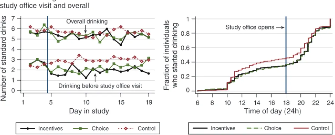
The impacts of sobriety incentives on overall alcohol consumption were con-siderably smaller than the impacts on daytime drinking, implying that subjects who responded to the incentives mostly shifted their alcohol consumption to later times of the day rather than reducing their overall consumption or not drinking at all. Panel A of Figure 4 shows the evolution of reported number of drinks before coming to the study office and overall. While the incentives reduced drinking before study office visits significantly, the impact on overall drinking was consid-erably smaller.20 Consistent with these results, the incentives caused a shift in the
distribution of the timing of individuals’ reported first drink of the day (panel B of
17 The decline in sobriety in the Control Group over the course of the study is in part explained by the lower overall attendance in all treatment groups. In addition, individuals may have felt more comfortable visiting the study office inebriated or drunk at later stages of the study.
18 Whether an individual in the Choice Group received incentives was determined by the choice that was ran-domly selected to be implemented for this individual. Choice 1 was implemented 90 percent of the time, such that the fraction of individuals in the Choice Group who actually received incentives closely tracked the fraction of individuals who chose incentives over Rs 90.
19 These discussions assume that self-imposed and externally imposed incentives were equally effective, which may not have been the case. For instance, external incentives may have decreased intrinsic motivation to stay sober (Bénabou and Tirole 2003).
20 Notably, overall drinking in the Control Group was already slightly higher on days 2 to 4, i.e., before the incentives to remain sober were assigned.
Figure 4). About 10 percent of the individuals in the Incentive and Choice Groups delayed the time of their first drink from between 10 am and noon to the evening. Importantly, however, individuals in the Incentive and Choice Groups did not arrive at the study office earlier than individuals in the Choice Group. In fact, on aver-age, individuals in the Incentive Group visited the study office a few minutes later (online Appendix Table A.7).
These visual impressions are confirmed by the regression results (panel B of Table 3). First, both treatments reduced reported overall alcohol consumption by about 0.3 standard drinks per day, about one-third of the effect on the reported num-ber of drinks before coming to the study office as described above. None of these estimates are statistically significant. Second, the reduction at the extensive margin of drinking was small at best. The point estimate for the pooled treatment effect sug-gests a 2 percentage point increase in reported abstinence from drinking altogether on any given day, but none of the estimates are statistically significant. Third, the treatment effect on reported overall alcohol expenditures is a reduction of about Rs 9 per day, with a point estimate of Rs 8.8 for the pooled treatment effect.
C. The Impact of Increased Sobriety on Labor Market Outcomes
Alcohol consumption has long been hypothesized to interfere with individuals’ ability to earn income, yet well-identified causal evidence is scarce (Cook and Moore 2000).21 While positive, I estimate the effect of sobriety incentives on earnings to be
21 Irving Fisher (1926) was among the first to investigate the relationship between alcohol and productivity. Based on small-sample experiments by Miles (1924) that showed negative effects of alcohol on typewriting efficiency, Fisher (1926) argued that drinking alcohol slowed down the “human machine.” He also argued that industrial efficiency was one of the main reasons behind the introduction of alcohol prohibition in the United States. While many studies since Fisher (1926) have considered the relationship between alcohol consumption, income, and productivity (for an
Drinking before study office visit Overall drinking 0 1 2 3 4 5 6 7
Number of standard drinks 1 5 10 15 19
Day in study Panel A. Drinking before study office visit and overall
Study office opens
0 0.2 0.4 0.6 0.8 1
Fraction of individuals who started drinking
6 8 10 12 14 16 18 20 22 24
Time of day (24h) Panel B. Time of first drink
Incentives Choice Control Incentives Choice Control
Figure 4. The Impact of Incentives on Day Drinking and Overall Drinking Notes: This figure shows the impact of the two sobriety treatments on drinking patterns.
• Panel A shows the self-reported number of standard drinks consumed before the study office visit and the
overall number of standard drinks consumed per day.