HAL Id: lirmm-00798708
https://hal-lirmm.ccsd.cnrs.fr/lirmm-00798708
Submitted on 5 Apr 2019HAL is a multi-disciplinary open access
archive for the deposit and dissemination of sci-entific research documents, whether they are pub-lished or not. The documents may come from teaching and research institutions in France or abroad, or from public or private research centers.
L’archive ouverte pluridisciplinaire HAL, est destinée au dépôt et à la diffusion de documents scientifiques de niveau recherche, publiés ou non, émanant des établissements d’enseignement et de recherche français ou étrangers, des laboratoires publics ou privés.
Tree mining: Equivalence classes for candidate
generation
Federico del Razo Lopez, Anne Laurent, Pascal Poncelet, Maguelonne
Teisseire
To cite this version:
Federico del Razo Lopez, Anne Laurent, Pascal Poncelet, Maguelonne Teisseire. Tree mining: Equiva-lence classes for candidate generation. Intelligent Data Analysis, IOS Press, 2009, 13 (4), pp.555-573. �10.3233/IDA-2009-0381�. �lirmm-00798708�
DOI 10.3233/IDA-2009-0381 IOS Press
Tree mining: Equivalence classes for
candidate generation
F. Del Razo L´opeza, A. Laurentb, M. Teisseireband P. Ponceletb
aToluca Institute of Technology – ITT, Av. Instituto Tecnol´ogico S/N – Col. Ex-Rancho La Virgen,
Metepec, Edo. de M´exico C.P. 52140, M´exico
bUniversity Montpellier 2 – LIRMM, 161, rue Ada, Montpellier, France
E-mail: {laurent,teisseire, poncelet}@lirmm.fr
Abstract. With the rise of active research fields such as bioinformatics, taxonomies and the growing use of XML documents,
tree data are playing a more and more important role. Mining for frequent subtrees from these data is thus an active research problem and traditional methods (e.g., itemset mining from transactional databases) have to be extended in order to tackle the problem of handling tree-based data. Some approaches have been proposed in the literature, mainly based on generate-and-prune methods. However, they generate a large volume of candidates before pruning them, whereas it could be possible to discard some solutions as they contain unfrequent subtrees. We thus propose a novel approach, called pivot, based on equivalence classes in order to decrease the number of candidates. Three equivalence classes are defined, the first one relying on a right equivalence relation between two trees, the second one on a left equivalence relation, and the third one on the ground of a root equivalence relation. In this paper, we introduce this new method, showing that it is complete (i.e., no frequent subtree is forgotten), and efficient, as illustrated by the experiments led on synthetic and real datasets.
Keywords: Data mining, tree mining, candidate generation, equivalent classes
1. Introduction
Tree data are playing a more and more important role for instance in the data exchanges (i.e. XML is now a standard format) or for scientific data which are often based on trees (e.g. biology). The extraction of frequent substructures, also known as tree mining, from huge tree databases is thus an active and important problem addressed by researchers from the data mining community [2,6,11,12,17]. In this context, a subtree is said to be frequent if it appears in more than σ trees from the database, where σ is called the minimal support. Frequent subtrees are very informative and they can be used to help the user or the system to be aware of what occurs in the database (for instance to discover knowledge for phylogenetic, or to mine for mediator schemas). However, it has been shown that regular data mining techniques such as algorithms extracting frequent itemsets from transactional data are not appropriate for tree mining since the data being considered are much more complex. Researchers have thus developed several methods to tackle the problem. These methods are based on the well-known level-wise generate-and-prune methods: first, candidates are generated, then they are afterwards tested to discard non frequent candidates and used to build new bigger candidates. Those propositions address several problems: (i) the representation of tree data has to be as efficient as possible (time and memory), (ii) the definition of tree inclusion, (iii) the generation of candidates and (iv) the validation of frequent candidates.
All the methods proposed in the literature suffer from the large number of candidates generated whereas some of them could be discarded before being validated over the database. As the step consisting in counting in how many trees from the database a subtree is included is very time-consuming and memory-consuming, it is mandatory to decrease the number of candidates in order to remain scalable.
In previous works, we have defined an efficient representation of the tree data structure and an optimized support counting method [7,8]. In this paper, we focus on the step of candidate generation. Our approach is based on equivalence classes, which are based on a pivot tree which acts as a representative (typical of each equivalence class). Three kinds of equivalence classes (and thus three kinds of pivots) are considered: left, right and root. A left pivot tree (resp. right), for a tree T , corresponds to the tree composed by all the nodes but the most-left leaf (resp. right) of T . The equivalence relations, which these classes are based on, will be detailed later on in this paper.
A tree where the root has no more than one child is called a root pivot. Each set of trees having k nodes is associated with the set of pivots that are necessary to build the equivalence classes. From these classes, it is then easy to build candidates having k + 1 nodes by combining two trees sharing the same pivot. Roughly speaking, the method is the same as Apriori-like methods [1] where the pivot of size k− 1 is completed by the two specific items (here nodes) in order to build a k + 1-node tree. By using this approach, we decrease the number of candidates as we guarantee that no subtree which will be non frequent will be generated. Moreover, we show that our approach is complete, as we generate all the frequent subtrees.
This paper is organized as follows. Section 2 recalls the basic definitions concerning trees. Section 3 presents existing work, mostly focusing on how candidates are generated. Section 4 introduces our approach pivot and demonstrates its completeness. Experiments are reported in Section 5. Finally, Section 6 concludes the paper.
2. Basic definitions
A rooted tree T is an undirected, connex and acyclic graph, with a special node r called the root of T , and denoted by root(T ). We say that T is labelled if each node have assigned a symbol from an alphabet Σ and we say that T is ordered if a left-to-right order among siblings in T is given. All trees in this paper are rooted, labelled and ordered. Formally a tree T is defined as a five-tuple T = (V, E, r,≼, L) where: i) V is a finite set of nodes, ii) E⊂ V × V is a binary relation of parentage between the nodes from T , iii) r is the root of T , iv)≼⊆ V × V is a sibling relation of the children of each internal node n ∈ V , and v)L: V → Σ is the labelling function for the nodes in V . The degree of a node u ∈ V is defined by the size of its neighborhood, such as deg(u) =|E(u)|. The size of T is |V |.
A path from node u1 to node ukis a sequence of nodes and edges (u1, e1, u2, e2, . . . , ek−1, uk) in T
such as ei = (ui, ui+1) for all i < k and u1 ̸= uk. As an edge can only be defined by its initial and
final nodes, the path from u1 to uk can be simply given by the succession of nodes (u1, u2, . . . , uk)
included in the path. The path is denoted by (u1, uk). The length of a path is the number of edges in the
succession.
The transitive closure E+of the parentage between the nodes belonging to T are defined by: E0= {(u, u)|u ∈ V };
En+1= {(u, w)|∃v ∈ V : (u, v) ∈ E ∧ (v, w) ∈ En}; for n! 0, and
{a, b, c} T r a a b b c c 1 2 3 4 5 6
Fig. 1. A preorder numerated tree.
E+= !
n>0
En.
Given a rooted, ordered, labelled tree (a tree for short) T the following relations can be defined depending on the unique path (r, u), from the root of T to all node u∈ V .
The parent of a node v∈ V \ {r} is the node being the source of the edge (u, v) such as parent(v) = {u ∈ V |(u, v) ∈ E}. The root has no parent: parent(r) = ∅. For an edge (u, v) ∈ E, u is said to be the parent of v, and v the child of u. The set of children of a node u ∈ V is denoted children(u) ={v ∈ V |(u, v) ∈ E}. If children(u) = ∅, the node u is a leaf.
The ancestors of a node v ∈ V \ {r} are all the nodes from path (r, v) but v. The set of the ancestors of a node v is denoted by ancestors(v) = {u ∈ V |(u, v) ∈ E+}. If u is an ancestor
of v, then v is said to be a descendant of u. The set of all the descendants of u is denoted by: descendants(u) ={v ∈ V |(u, v) ∈ E+}.
A node u is a sibling of a node v∈ V \ {r} if it shares the same parent: parent(u) = parent(v). The set of siblings of a node is denoted siblings(u) ={v ∈ V |parent(u) = parent(v)}.
If the nodes u, v, y ∈ V \{r} and w ∈ V are considered, together with a parentage relation (w, u) ∈ E, then it is possible to distinguish between the children of a node: given u, v∈ V , the node u is the
left-most-child of w, denoted by f irst(w), if f irst(w) = {u|!v, (w, v) ∈ E ∧ v < u}. The node v is the right-most-child of w, denoted by last(w), if last(w) = {v|!u, (w, u) ∈ E ∧ v < u}. We say that the node v is the next-sibling of node u, denoted by next(u), if next(u) = {v|(w, v) ∈ E ∧ u < v ∧ !y such as (w, y) ∈ E ∧ u < y < v}. The node u is the previous-sibling of v, denoted by previous(v), if next(v) ={u}.
The left-most-branch of T , denoted by lmb(T ), corresponds to the path (v1, v2. . . , vk), where v1 = r
such that f irst(vi−1) = {vi}, ∀i, 2 " i " k. The final node vkin lmb(T ) is called left-most-leaf and it
is denoted by lml(T ).
The right-most-branch of T , denoted by rmb(T ), corresponds to the path (v1, v2. . . , vk), where
v1 = r such that last(vi−1) = {vi}, ∀i, 2 " i " k. The final node vkin rmb(T ) is called right-most-leaf
and is denoted by rml(T ).
Example 1. Figure 1 shows a tree T with its root r, the set of nodes V = {1, 2, 3, 4, 5, 6}, and the
relations between the nodes:
E ={(1, 2), (1, 3), (3, 4), (3, 5), (3, 6)} E+= {(1, 2), (1, 3), (3, 4), (3, 5), (3, 6),
Here we have the following relationships: parent(6) = {3}, children(3) = {4, 5, 6}, ancestors
(6) = {3, 1}, descendants(1) = {2, 3, 4, 5, 6}, siblings(4) = {5, 6} first(3) = {4}, last(3) = {6}, next(2) ={3}, previous(3) = {2}, lmb(T ) = (1, 2), rmb(T ) = (1, 6), lml(T ) = {2} and rml(T ) = {6}.
Considering a tree T = (V, E, r,≼, L), a tree S = (V′, E′, u,≼′,L′) is said to be a subtree of T if u ∈ V and V′ = u " descendant(u) and E′ = V′× V′ and≼′⊆ V′× V′such that (v, v′) ∈≼′ ⇐⇒
(v, v′) ∈≼ and L′is the restriction ofL from V to V′.
2.1. Tree mining
Given a tree database D ={T1, . . . , Tn}, we say that a subtree S is supported by a tree T ∈ D if S is
a subtree of T . Then the support of S with respect to a tree T is given by:
supp(S, T ) = ⎧ ⎨ ⎩ 1, if S is a subtree of T 0, otherwise
The support of S with respect to a database D is defined as supp(S, D) =
&
Ti∈Dsupp(S, Ti) |D|
If supp(S, D) is greater or equal to a user-defined threshold σ, then subtree S is considered frequent. Otherwise S is said to be an infrequent subtree. Given a tree database D and a minimum support σ (0" σ " 1), the goal of tree mining is to find the collection of frequent subtrees in D.
3. Related work
In this section, we give a short survey of the existing approaches, focusing on the generation of candidates.
To efficiently extract frequent subtrees, the methods introduced in [2–5,12,16,17] use the so-called level-wise approaches. At each step of the algorithm, candidate trees are generated based on the ones that have been found frequent at the previous step. The k level thus refers to the step where trees of size k(k nodes) are being treated. These trees are then tested on the database in order to count the number of trees they are included in. This number corresponds to the support value.
In the existing methods, the step of tree generation if thus critical as every frequent subtree must be proposed as a candidate in order to be complete, whereas it is decisive to generate as few candidates as possible in order to remain scalable.
Existing approaches consider that the generation of candidates is done by extending the right most branch [3–5,13,17]. The trees are numbered in a depth-first enumeration: for every tree T having k nodes, we have root(T ) = 1 and rml(T ) = k. F denotes the set of frequent trees and Fkdenotes the
set of frequent trees having k nodes (for every k,Fkis a finite set). The generation of candidates relies
on equivalence classes as all the trees having k nodes are represented by the depth-first enumeration and are then grouped based on the equivalence relation has same k− 1 prefix. Two trees belonging to the same equivalence class only differ in the last node (position and label).
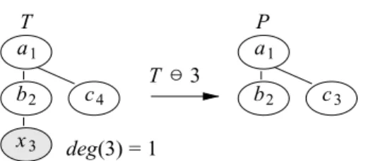
P T T 3 deg(3) = 1 a a b c b c x 1 1 2 2 3 3 4
Fig. 2. Pivot P obtained by removing the left most leaf rml(T ) from T .
It is easy to show that this method is complete. However, this method leads to a large number of non frequent candidates. In order to limit the number of candidates, existing approaches rely on the so-called anti-monotonicity property [10] claiming that if a tree is non frequent, then every super-tree will be non frequent as well. In the case of trees, such a naive pruning is far too time-consuming. In order to tackle this problem, we thus propose to reduce the number of trees being generated instead of generating candidates and then pruning them.
gSpan [13] can be viewed as similar to our approach, as: 1) it handles graphs, 2) it considers the enumeration of graphs by using the right-most extension, 3) the methods are based in the Pattern-growth approach for the generation of candidates to avoid duplicates.
However there are differences that prevent from comparing these methods. First of all, the algorithm gSpan defines a labeled graph as G = (V, E,L) whereas, PIVOT defines a Tree (graph) as T = (V, E, r, ≼, L), where there cannot exist any cycle. In other words, gSpan is designed to work with a more general model including: trees, lattices, sequences, whereas our approach is particularly aimed at working with rooted, labeled and ordered trees. Second, it should be noted that to validate the graph inclusion, gSpan is based on the isomorphism definition validating vertices and edge labels, whereas the method proposed here (PIVOT) is based on the inclusion test of nodes, label nodes, vertices, edges and the sibling order relation.
4. The pivot method
In this section, our pivot method is introduced. This method allows us to combine equivalence classes (left, right and root) to generate candidates.
4.1. Definitions
This section aims at introducing the⊖ and ⊕ operators, which our approach relies on.
Definition 1 (Deletion). Given a tree T such as size(T ) = k and u∈ V such as deg(u) = 1, we define
the⊖ operator on the trees such as T ⊖ u returns the subtree P of size k − 1 included in T from which the node u has been deleted. The subtree P is called the pivot. Figure 2 illustrates how⊖ works.
Remark: The⊖ operator can not be applied on trees where the degree of the root node to be deleted equals 1 to avoid two trees as a result.
Definition 2 (Insertion). Given a tree T and a pair (p, l), 1" p " k, the ⊕ operator is such that: – T ⊕ (p, l) inserts a new node with label l as the last child of the node being at position p in T , – (p, l)⊕ T inserts a new node with label l as first child to the node being at position p in T .
. T (1, x ) T a a b b c x c 1 1 2 2 3 3 4
(a) left insertion
. T (1, x ) a a b c b c x 1 1 3 2 2 3 4 (b) right insertion Fig. 3. Insertion of a new node in tree T .
4.2. Right equivalence class
LetFk be the set of frequent trees having k nodes and two k-trees F, F′ ∈ Fk. Given a tree F , the
function δ(F ) = F ⊖ rml(F ) returns a pivot subtree Pδ of size k− 1. This function defines the right
equivalence relation, denoted byPδ, as FPδF′⇐⇒ δ(F ) = δ(F′)
Note that it is trivial to show thatPδis an equivalence relation as it relies on an equality. The relation
Pδ is thus reflexive, symmetrical and transitive. Trees F and F′ belong to the same right equivalence
class if and only if they share a common structure at position k− 1. We denote [Pδ(F )] the right
equivalence class of F defined by: Pδ(F ) = {F′ ∈ Fk|F PδF′}
Given a set of treesF, we recall that the quotient set of F by the equivalence relation Pδcorresponds
to the set of the equivalence classes ofF depending on Pδ (i.e. the set{[Pδ(F )]|F ∈ F}). Note that
every tree F ∈ F belongs to one and only one equivalence class. It can thus be represented by its right pivot associated with the right most leaf (position and label) that distinguishes it from the other trees belonging to the same class.
In the following we note an equivalence class corresponding to a pivot by the notation [PX] where
P stands for the pivot and X differs from the different equivalence classes. A right equivalence class [Pδ], sharing a common pivot subtree, can be represented as a pivot tree Pδ together with a
list R = {R[1], . . . , R[|R|]} of pairs (R[i]1, R[i]2) corresponding to every tree F ∈ F such that
F⊖ rml(F ) = Pδwhere R[i]1(i∈ [1, |R|]) corresponds to the position rml(F ) and R[i]2corresponds
to the label of rml(F ). We thus have: [Pδ] ∼ {Pδ, R}
4.2.1. Generation of candidates regardingPδ
Definition 3 (Product). Given a right equivalence class [Pδ] ∼ {Pδ, R} and two trees F, F′ such that
FPδF′, and considering (p, l), (p′, l′) two pairs in R such that F = Pδ⊕ (p, l) and F′ = Pδ⊕ (p′, l′),
then⊗ operator is defined [14] to build a new [F ] right equivalence class. The ⊗ operator is applied on each pair in R such that:
– if (p == p′) then
[F ].R+ = {(l′, parent(rml(F ))), (rml(F ), l′)} – if (p > p′) then
3 F1 F2 F3 a a a b b c d c d 1 1 1 2 2 2 3 3 3
Fig. 4. Frequent trees of size 3.
(F1) (F2) (F3) P1 P2 a a a b c b 1 1 1 2 2 2
Fig. 5. Right pivots.
At each step (level) k of the algorithm, the candidates of level k + 1 are generated by computing the product of all the pairs of elements of size k− 1 in each equivalence class (for the pairs that share their k− 2 first nodes). All the combinations of compatible trees (regarding the right pivot) are thus obtained.
Remark: Existing approaches, such as [3,4,17], considering an extension by the right most branch,
can be represented by means of⊗. However, the use of a single equivalence relation for generating the candidates leads to the generation of a large number of candidates containing at least one non frequent subtree, which should thus be discarded. We propose to combine several equivalence relations in order to decrease the number of candidates being generated.
We thus rely on the right equivalence relation defined above, but also on a left equivalence relation and a root equivalence relation, as described below.
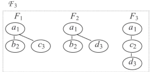
Example 2. Let us consider the set of frequent trees of size 3, denoted by F3, depicted on Fig. 4.
We apply the function δ on the set F3 by eliminating the right most leaf from each tree such that :
δ(F1) = F1⊖ rml(F1), δ(F2) = F2⊖ rml(F2) and δ(F3) = F3⊖ rml(F3). As δ(F1) = δ(F2), then it
is a common pivot denoted by Pδ1. Moreover, the pivot obtained from F3 is identified by Pδ2. The pivot
trees Pδ1 and Pδ2 are shown on Fig. 5. These pivot trees allow us to build the following equivalence
classes:
[Pδ1] ∼ {Pδ1,{(1, c), (1, d)}} [Pδ2] ∼ {Pδ2,{(2, d)}}
Note that the first class [Pδ1] regroups the frequent trees F1 and F2that can be built from the (p,
l)-extensions (1, c) and (1, d), meaning that F1 = Pδ1 ⊕ (1, c) and F2 = Pδ1⊕ (1, d).
The product operator⊗ applied on the pairs from the class [Pδ1] generates the following two classes: [F1] ∼ {F1,{(1, c), (3, c), (1, d), (3, d)}}
P 1 P 2 F1 F1 F1 F1 F2 F2 F2 F2 F3 F3 [F1] [F2] [F3] C1 C2 C3 C4 C5 C6 C7 C8 C9 C10 a a a a a a a a a a a a b b b b b b b b b c c c c c c c c c c c d d d d d d d d d d d d 1 1 1 1 1 1 1 1 1 1 1 1 2 2 2 2 2 2 2 2 2 2 2 2 3 3 3 3 3 3 3 3 3 3 4 4 4 4 4 4 4 4 4 4
Fig. 6. Candidate trees generated by the product operator applied on the class [Pδ1] and [Pδ2].
The equivalence class which has F3as common pivot is obtained by applying the product operator on
the pairs from [Pδ2].
[F3] ∼ {F3,{(2, d), (3, d)}}
The candidates C1, C2, . . . , C10 given by Fig. 6 result from the combination of the pivot on each
equivalence class [F1], [F2] and [F3] with each pair from the list R in these classes. Thus, the candidate
tree C1is generated by C1= F1⊕ (1, c), and C2 = F1⊕ (3, c), and so on.
(F1) (F3) (F2) P 1 P 2 a a a c d c 1 1 1 2 2 2
Fig. 7. Left pivot trees.
non-valid candidates (which one knows they will not be frequent). We can see that only the candidates C4
and C9in Fig. 6 are valid because inside the others candidates, there is a subtree of size 3 (in bold) which
does not belong to 3-frequent subtrees setF3(cf. Fig. 4). Then, by the property of anti-monotonicity, we
know a priori that these trees are not frequent. We thus propose to rely on several relations of equivalence in order to reduce the number of candidates generated while preserving a complete approach. We use at the same time the right, left and root relations of equivalence. We thereby propose a strategy of generation of candidates based on three equivalence classes allowing to handle a subset of candidates more restricted but complete.
4.3. Left equivalence classes
Given two k-trees F, F′ ∈ Fk, we define a function ω(F ) = F ⊖ lml(F ) to get the pivot subtree Pω
and we define a left equivalence relationshipPωas
FPωF′ ⇐⇒ ω(F ) = ω(F′)
Trees F and F′belong to the same left equivalence class if and only if they share the same common structure to the position k− 1. The left equivalence class of a tree F is defined by:
Pω(F ) = {F′∈ Fk|F PωF′}
As for the right equivalence classes, every tree F ∈ F belongs to one and only one left equivalence class and can be represented by its left pivot Pω = F ⊖ lml(F ) and a pair (p, l) corresponding to the
position p and the label l of its left most leaf lml(F ). We can thus represent a left equivalence class [Pω] by a pivot Pωand a list L ={L[1], . . . , L[|L|] where L[i]1(i∈ [1, |L|]) corresponds to the position
lml(F )and L[i]2corresponds to the label of lml(F ). We thus have:
[Pω] ∼ {Pω, L}
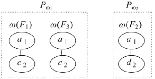
Example 3. By applying the function ω on the trees from Fig. 4 we get the pivots ω(F1) = F1⊖ rml(F1),
ω(F2) = F2 ⊖ rml(F2) and ω(F3) = F3⊖ rml(F3) illustrated by Fig. 7. As ω(F1) = ω(F3), it is a
common pivot identified by Pω1. The pivot δ(F3) is denoted by Pω2. These pivot trees allow us to group
together the trees belonging toF3in the following equivalence classes:
[Pω1] ∼ {Pω1,{(1, b), (2, d)}} [Pω2] ∼ {Pω2,{(1, b)}}
(F1) (F2) (F3) P 1 P 2 0 c d 1 2 /
Fig. 8. Root pivot trees.
4.4. Root equivalence classes
Let γ(F ) be a function which removes the root from tree F of size k and returns the pivot tree Pγof
size k− 1. γ(F ) is defined by:
γ(F ) =' F ⊖ root(F ), if |children(root(F ))| = 1 ∅, otherwise
Note that if we allow γ(F ) to be applied on the trees which root has a degree greater then 1, then this function will return a forest of trees (where each tree size will be lower than (k− 1). In order to avoid the operations between the trees and the forests, we set that γ(F ) =∅ if |children(root(F ))| ̸= 1.
Given two k-root trees F, F′ ∈ F
k, we define the root equivalence relationPγas follows:
FPγF′⇐⇒ γ(F ) = γ(F′)
The root equivalence class is defined by:
Pγ(F ) = {F′ ∈ Fk|F PγF′}
An equivalence class which pivot tree is Pγis denoted by [Pγ]. Each tree F ∈ Fkbelongs to one and
only one equivalence class [Pγ]. A root equivalence class [Pγ] can then be represented by a pivot tree
Pγ and a list of pairs O = {O[1], . . . , O[|O|]}. Each pair O[i] corresponds to the root which has been
removed from a tree F . As done above, a root equivalence class [Pγ] can be given by its root pivot Pγ
together with a list of pairs (position,label). We thus have [Pγ] ∼ {Pγ, O}
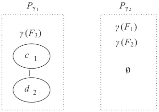
Example 4. Figure 8 illustrates the pivot trees γ(F1) = γ(F2) = ∅ and γ(F3) = F3⊖ root(F3) obtained
fromF3(cf. Fig. 4). As a consequence, we can build the equivalence classes:
[Pγ1] ∼ {Pγ1,{(−1, c)}} [Pγ2] ∼ {∅, {∅}}
P1 P2 P3 P4 a a a b c c d d 1 1 1 1 2 2 2 2
Fig. 9. Pivot trees.
4.5. Grouping the equivalence classes
To obtain an equivalence class with a common tree P , we regroup the equivalence classes [Pδ], [Pω]
and [Pγ] in a new one denoted by P, defined by:
P(F ) = {F′ ∈ Fk|F PδF′∨ F PωF′∨ F PγF′}
and represented by: [P ] ∼ {P, R, L, O}
where P is a pivot tree, R (resp. L) is a list containing the right most leaves (resp. left most leaves) removed from the frequent trees by function δ(F ) (resp. ω(F )) and O is a list containing all the roots removed by the function γ(F ). The list of equivalence classes [P ] are filled in following the criteria below:
– if FPδF′then the pair (position, label) is added to list R – if FPωF′ then the pair (position,label ) is added to list L – if FPγF′then the pair (position, label) is added to list O
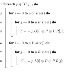
The Algorithm 1 describes how to obtain the equivalence classes from the set of frequent subtrees of size k. In this algorithm, we use a hash table (line 1), denoted by H, in order to generate a pivot tree only once. From line 3 to line 13, the instructions are meant to deal with each frequent tree from F . Firstly, we verify whether the degree of the root is equal to 1 in order to avoid the creation of a forest. If yes, then the root of F is removed. Then, we use the resulting pivot S1as hash key in H and the root is added
to the list O in the equivalence class. Secondly, the left most leaf is removed from F , resulting in pivot S2, which is used as hash key while the removed leaf is added in L. Note that a pair (position, label) is
added to list L. Thirdly, the pivot S3is obtained by removing the right most leaf, which is added to R.
Finally, the pivot method is called to build the candidate trees.
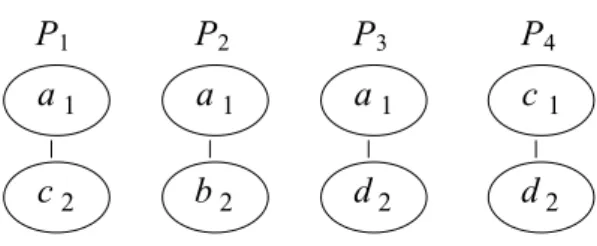
Example 5. Let us consider the frequent trees from Fig. 4 to build the classes having a common pivot
P. In the first tree F1, the root cannot be removed. So the leaf with number 2 is removed, leading to the
pivot P1 illustrated by Fig. 9. This tree will serve as a basis to build the class [P1] and the pair (1, b)
is added to its list L such that: [P1] ∼ {P1, R =∅, L = {(1, b)}, O = ∅}. Coming to F1, by removing
leaf 3, we get a new pivot identified by P2 in Fig. 9. On the contrary to the previous case, we add the
pair (1, c) to the list R such that: [P2] ∼ {P2, R ={(1, c)}, L = ∅, O = ∅}. The trees in F2and F3are
treated in the same way to obtain the following classes:
[P1] ∼ {P1, R ={(2, d)}, L = {(1, b), (2, d)}, O = ∅}
Algorithm 1: GenCandPivot
[P3] ∼ {P3, R =∅, L = {(1, b)}, O = ∅}
[P4] ∼ {P4, R =∅, L = ∅, O = {(−1, a)}}
4.6. The pivot algorithm
Candidates of size k + 1, denoted byCk+1, are generated from the combination of elements coming
from the equivalence classes built from the k frequent trees and that share a common pivot of size k− 1 (cf. Algorithm 2).
First (lines 2–5), pairs from right and root classes are combined to generate the following set of candidatesCk+1γ :
Algorithm 2: Pivot: Generating candidates P1 P1 C1 C2 a a c c d d d d 1 1 2 2 3 3 4 4
Fig. 10. Candidates obtained by pivot.
Then (lines 6–8), we consider the pivot P . All the combinations between one element from the right list and one from the left list are combined to generate the next set of candidatesCω
k+1
Ck+1ω = {L[i] ⊕ P ⊕ R[j]: i ∈ [1, |L|] and j ∈ [1, |R|]
Finally, the set of all candidates is generated from the union of two subsets of candidates generated from breadth (left + right) and depth (root + right):
Ck+1 = Ck+1ω
! Ck+1γ
Example 6. Figure 10 illustrates the candidates obtained by combining the elements from the classes
[P1], . . . , [P4]. With class [P1], the candidate C1 is generated with the first element from the left list L
combined with the single element from R: C1= (1, b) ⊕ P1⊕ (2, d). The second candidate is obtained
root list O is empty, it is not possible to build candidates from R combined with O. For [P1], [P2] [P3],
no candidate is generated (either R is empty or L and O are empty).
Note that using the Zaki methods, 10 candidates are generated with a single equivalence class whereas Pivot generated only 2 of them ( cf. Fig. 6).
We demonstrate here that all the frequent subtrees are discovered and generated as candidates.
Theorem 1. The PIVOT method allows us to extract all frequent subtrees.
Proof 1. Let us consider that the counting algorithm is correct. We have to prove that each frequent
subtree has been generated as a candidate: ∀fk∈ F, fk∈ Ck.
This property is demonstrated recursively by considering the size k of the frequent subtree.
k = 1 The frequent subtrees of size 1 (nodes) are discovered by a scan of the database, as performed
by any other method. It is thus complete.
k = 2 The frequent subtrees of size 2 are discovered by combining in all possible manners the frequent
nodes, which is thus complete.
k > 2. Let us assume that all the frequent trees of size t" k have been extracted. Let us demonstrate
that every tree of size k + 1 is generated as a candidate.
Let us consider fk+1∈ Fk+1, every subtree of fk+1is thus frequent.
Moreover, it is easy to show that for every tree t having at least 3 nodes, first deleting the right most leaf and then the left most leaf or, on the contrary, first deleting the left most leaf and then the right most leaf is the same.
Similarly, if the tree is a root tree, first deleting the root and then the right most leaf or first deleting the right most leaf and then the root is the same:
(t ⊖ lml(t)) ⊖ (rml(t ⊖ lml(t))) = (t ⊖ rml(t)) ⊖ (lml(t ⊖ rml(t))) (t ⊖ lml(t)) ⊖ (root(t ⊖ lml(t)))
= (t ⊖ root(t)) ⊖ (rml(t ⊖ root(t)))
Thus, the right pivot of the left pivot of a tree t is the same as the left pivot of the right pivot.
As a consequence, these trees are combined by our approach as the trees are obtained by computing the cartesian product of the trees from the equivalence classes Γ and ∆ from the one hand and Ω and ∆ from the other hand.
In this framework, two cases can occur: a breadth-expansion or a depth-expansion:
If there exists f ∈ fk+1 of size k such that depth(f ) = depth(fk+1). Then we denote by fk1 =
fk+1− rml(fk+1) and fk2 = fk+1− lml(fk+1) the two frequent trees found by deleting the right
most leaf and left most leaf. As mentioned previously, the pivot of the left equivalence class of fk1
(f1
k⊖ lml(fk1)) is equal to the pivot of the right equivalence class of fk2(fk2⊖ rml(fk2)).
Thus fk1et fk2are combined by our method, leading to fk+1by a breadth-expansion.
Otherwise there must exist a tree f of depth depth(fk+1) − 1 such that f is frequent as every
subtree is frequent. We consider f3
k = fk+1 − root(fk+1) and fk4 = fk+1 − rml(fk+1) with
depth(f3
k) = depth(fk+1) − 1.
The right pivot droit of fk3is equal to the root pivot of fk4. There thus exists a right equivalence class at step k− 1 with the same pivot as on root equivalence class, leading to the generation of fk+1par
depth-expansion when the cartesian product will be computed.
Table 1
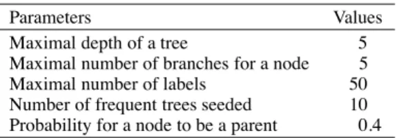
Parameters to build the synthetic dataset
Parameters Values
Maximal depth of a tree 5
Maximal number of branches for a node 5
Maximal number of labels 50
Number of frequent trees seeded 10 Probability for a node to be a parent 0.4
1 10 100 1000 0.01 0.1 1 Number of Trees Support (%) |DBsynt|=100K Pivot vTreeMiner
(a) Frequent trees
100 1000 10000 0.01 0.1 1 Number of Trees Support (%) |DBsynt|=100K Pivot vTreeMiner (b) Candidates
Fig. 11. Number of trees on synthetic data (embedded inclusion).
5. Experiments
The experiments were performed on a Pentium 1400 Mhz, 256 Mb RAM and 1024 Kb cache memory, running Linux 2.6 with C++ and STL data structures compiled with gcc 4.0.
5.1. Synthetic data
vTreeMiner has been chosen as a reference as it is based on Apriori, using the source code delivered by
Zaki [15]. As our source code and this one have been developed under the same programming language, we were able to use the same function gettimeofday() to measure runtimes and the function mallinfo() to measure the memory consumption.
We generated a database using method proposed in [12]. The parameters used to generate these datasets are given in Table 1.
When considering embedded inclusion, meaning that ancestor-descendants are taken in account, we use the vTreeMiner algorithm. The support has been defined from 0.9 to 0.01.
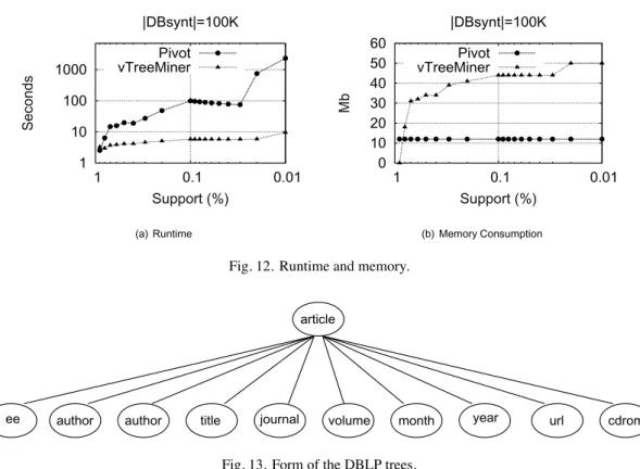
Figure 11(a) reports the number of frequent trees found using Pivot and vTreeMiner algorithms. The generation of candidates are very close between vTreeMiner and Pivot, (cf. Fig. 11(b)). The scopes used by vTreeMiner help it to get better runtimes (cf. Fig. 12(a)). However, it is more memory-consuming (cf. Fig. 12(b)).
1 10 100 1000 0.01 0.1 1 Seconds Support (%) |DBsynt|=100K Pivot vTreeMiner (a) Runtime 0 10 20 30 40 50 60 0.01 0.1 1 Mb Support (%) |DBsynt|=100K Pivot vTreeMiner (b) Memory Consumption
Fig. 12. Runtime and memory.
article
ee author author title journal volume month year url cdrom
Fig. 13. Form of the DBLP trees.
5.2. Real data
We report here the results obtained from the DBLP1database available from [9]. This database offers
bibliographic information on major computer science journals and proceedings, containing 328,458 references. Each entry of the database is a tree describing a paper published in a DBLP linked conference or journal. Figure 13 shows the typical form of such trees.
The trees are obtained from the references. For instance, the reference below is transformed into the tree shown by Fig. 14:
<article key="journals/siamdm/CanteautCD00"> <author>Anne Canteaut</author>
<author>Pascale Charpin</author> <author>Hans Dobbertin</author>
<title>Weight Divisibility of Cyclic Codes, Highly Nonlinear Functions on F<sub>2<sup><i>m</i></sup></sub>,
and Crosscorrelation of Maximum-Length Sequences.</title> <pages>105-138</pages>
<year>2000</year> <volume>13</volume>
<journal>SIAM Journal on Discrete Mathematics</journal> <number>1</number>
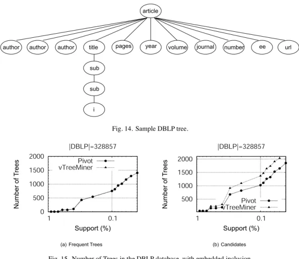
article author author author title sub sub i
pages year volume journal number ee url
Fig. 14. Sample DBLP tree.
Fig. 15. Number of Trees in the DBLP database, with embedded inclusion.
<ee>http://epubs.siam.org/sam-bin/dbq/article/35005</ee> <url>db/journals/siamdm/siamdm13.html#CanteautCD00</url> </article>
We compare in this section the results obtained by using Pivot and vTreeMiner algorithms.
Figure 15(a) shows the validity of our algorithms as they all extract the same frequent trees. Figure 15(b) shows the evolution of the number of candidates depending on the support (ranging from 0.9 to 0.01). As shown here, Pivot generates less candidates than vTreeMiner.
Figure 16(a) reports experiments conducted in order to evaluate runtime executions. As we can notice, Pivot clearly outperforms vTreeMiner. Furthermore, we can observe that for support values lower than 0.09, the execution time of vTreeMiner increases very quickly. The Fig. 16(b) shows the memory consumption of both algorithms. As expected, according to the data representation, Pivot is less memory-consuming.
As can be seen from the experiments reported above, Pivot is very efficient regarding the memory consumpation and can even outperform existing methos regarding runtime. More specifically, when our approach is applied on wide trees, then it outperforms existing methods, while it is not adapted to deep trees.
Regarding real data (DBLP) that are based on quite wide trees, vTreeMiner runs faster than Pivot for minimal supports greater than 0.1. However, it should be noted that this is inverted when supports
10 100 1000 10000 0.1 1 Seconds Support (%) |DBLP|=328857 Pivot vTreeMiner (a) Runtime 0 200 400 600 800 1000 0.1 1 Mb Support (%) |DBLP|=328857 Pivot vTreeMiner (b) Memory Consumption
Fig. 16. Experiments on the DBLP database.
become lower than 0.1, and that vTreeMiner cannot compute the frequent subtrees when the support is lower than 0.03 as the memory is fully occupied and fails.
6. Conclusion
Tree mining is an active but complex data mining topic having numerous applications (e.g. phylogenic, extraction of mediator schema). Many methods have been proposed in the literature, usually based on level wise methods. In this framework, the generation of candidates is one of the key points to design scalable algorithms. However, most of the existing tree mining approaches consider simple candidate generations, by building k-node candidates from (k− 1)-node frequent subtrees which they extend by adding a single node to the right most branch.
In this paper, we thus introduce an original and efficient method for generating candidates in the context of tree mining. We propose to merge two (k− 1)-node frequent subtrees that share a pivot (i.e. a (k− 2) node tree) for building a k-node candidate, in the same way as itemsets are merged in the APriori framework.
By this way, a large number of candidates can be immediately discarded, which saves memory. We propose a new method Pivot combining several equivalence relations in order to decrease the number of candidates being generated. We rely on the right equivalence relation, but also on a left equivalence relation and a root equivalence relation. This method is proven to be complete and efficient (regarding experiments reported here).
Acknowledgments
The authors would like to thank M. J. Zaki (Department of Computer Science, Rensselaer Polytechnic Institute Troy, New York), for the source codes of vTreeMiner and hTreeMiner he provided to us.
References
[1] R. Agrawal and R. Srikant, Fast algorithms for mining association rules, in: Proc 20th Int Conf Very Large Data Bases,
[2] T. Asai, K. Abe, S. Kawasoe, H. Arimura, H. Satamoto and S. Arikawa, Efficient substructure discovery from large semistructured data, in: SIAM Int Conf on Data Mining, 2002.
[3] T. Asai, H. Arimura, T. Uno and S. Nakano, Discovering frequent substructures in large unordered trees, in: DOI
Technical Report DOI-TR 216, Department of Informatics, Kyushu University, 2003.
[4] Y. Chi, S. Nijssen, R. Muntz and J. Kok. Frequent subtree mining – an overview, Fundamenta Informaticae 66(1–2) (2005), 161–198.
[5] Y. Chi, Y. Xia, Y. Yang and R. Muntz, Mining closed and maximal frequent subtrees from databases of labeled rooted trees, IEEE Transactions on Knowledge and Data Engineering 17(2) (2005), 190–202.
[6] J.D. Knijf, Frequent tree mining with selection constraints, in: Proc of the 3rd Int Workshop on Mining Graphs, Trees
and Sequences (MGTS), 2005.
[7] A. Laurent, P. Poncelet and M. Teisseire, Fuzzy data mining for the semantic web: Building xml mediator schemas, in:
Fuzzy Logic and the Semantic Web, E. Sanchez, ed., Capturing Intelligence, Elsevier, 2006.
[8] F.D.R. Lopez, A. Laurent, P. Poncelet and M. Teisseire, Rsf – a new tree mining approach with an efficient data structure, in: Proceedings of the joint Conference: 4th Conference of the European Society for Fuzzy Logic and Technology (EUSFLAT 2005), 2005.
[9] D. of Computer Science & Engineering University of Washington. Xmldata repository, 2002. http://www.cs.washington. edu/research/xmldatasets/.
[10] J. Pei and J. Han, Constrained frequent pattern mining: A pattern-growth view, ACM SIGKDD 2(2), 2002.
[11] S. Tatikonda, S. Parthasarathy and T. Kurc, Trips and tides: new algorithms for tree mining, in: Proc 15th ACM Int Conf
on Information and Knowledge Management (CIKM), 2006.
[12] A. Termier, M.-C. Rousset, and M. Sebag. Treefinder, a first step towards XML data mining, in: IEEE Conference on
Data Mining (ICDM), 2002, pp. 450–457.
[13] X. Yan and J. Han, gspan: Graph-based substructure pattern mining, in: Proc of the IEEE International Conference on
Data Mining (ICDM), 2002, pp. 721–724.
[14] M. Zaki, Efficiently mining frequent trees in a forest, in: ACM-SIGKDD’02, 2002. [15] M.J. Zaki, Treeminer code, http://www.cs.rpi.edu/˜zaki/software/.
[16] M.J. Zaki, Efficiently mining frequent embedded unordered trees, Fundamenta Informaticae 65(1–2) (2005), 33–52. [17] M.J. Zaki, Efficiently mining frequent trees in a forest: Algorithms and applications, IEEE Transaction on Knowledge
![Fig. 6. Candidate trees generated by the product operator applied on the class [P δ 1 ] and [P δ 2 ].](https://thumb-eu.123doks.com/thumbv2/123doknet/13951042.452321/9.892.242.619.135.813/fig-candidate-trees-generated-product-operator-applied-class.webp)
