Publisher’s version / Version de l'éditeur:
Vous avez des questions? Nous pouvons vous aider. Pour communiquer directement avec un auteur, consultez la première page de la revue dans laquelle son article a été publié afin de trouver ses coordonnées. Si vous n’arrivez pas à les repérer, communiquez avec nous à [email protected].
Questions? Contact the NRC Publications Archive team at
[email protected]. If you wish to email the authors directly, please see the first page of the publication for their contact information.
https://publications-cnrc.canada.ca/fra/droits
L’accès à ce site Web et l’utilisation de son contenu sont assujettis aux conditions présentées dans le site LISEZ CES CONDITIONS ATTENTIVEMENT AVANT D’UTILISER CE SITE WEB.
COSMOL Conference 2020 North America, 2020-10-08
READ THESE TERMS AND CONDITIONS CAREFULLY BEFORE USING THIS WEBSITE. https://nrc-publications.canada.ca/eng/copyright
NRC Publications Archive Record / Notice des Archives des publications du CNRC :
https://nrc-publications.canada.ca/eng/view/object/?id=781020e3-9a89-4f04-99db-66d067c3d328 https://publications-cnrc.canada.ca/fra/voir/objet/?id=781020e3-9a89-4f04-99db-66d067c3d328
NRC Publications Archive
Archives des publications du CNRC
This publication could be one of several versions: author’s original, accepted manuscript or the publisher’s version. / La version de cette publication peut être l’une des suivantes : la version prépublication de l’auteur, la version acceptée du manuscrit ou la version de l’éditeur.
Access and use of this website and the material on it are subject to the Terms and Conditions set forth at
Evaluating suggested lengths used for cut-off planes using the
effective length calculation procedure
Evaluating Suggested Lengths used for Cut-off Planes using The Effective Length
Calculation Procedure.
A. T. Hayes1, M. Ghobadi1, T. V. Moore2
1. Research Officer, National Research Council, Ottawa, ON, Canada
2. Research Council Officer, National Research Council, Ottawa, ON, Canada
Introduction
As building codes become more stringent in terms of thermal performance of building envelopes, and higher insulated wall assemblies are becoming more common, the heat flow due to major thermal bridges can contribute a significant portion of the total heat transfer through a building façade (Ghobadi, Moore, & Lacasse, 2019). Thermal bridge is a term used to describe a feature within a building façade which facilitates the transport of thermal energy through the envelope at a higher rate compared to the surrounding construction (ISO 10211, 2017). Thermal bridges can be found where there are changes in material properties or geometries that result in discrepancies in material thicknesses. Thermal bridges within buildings to name a few, can be found around windows, slab edges and in repeating studs within a wall. With building designers working to increase the overall energy efficiency of buildings, having tools to quantify the thermal performance of building façade during the design stage of a building is important. In quantifying the thermal performance of a building envelope during the design phase, project teams are able to identify major thermal bridges, and possibly change or adapt their design to mitigate the effects of the thermal bridge.
There are different methods being used to quantify the thermal performance of building assemblies, including but not limited to, hand calculations (ASHRAE, 2017) (National Research Council Canada, 2011), Guarded Hot Box testing (ASTM, 2019), In-Situ testing and computer simulations (ISO 10211, 2017). However as building geometries become more complicated, using these methods to calculate the thermal performance of a building envelope can become time consuming, challenging and in some cases generate results that may not reflect the actual thermal performance of the assembly. As designers look to computer simulations to quantify the amount of energy lost through building envelopes the size of simulations can become a challenge with computational limitations. By partitioning the building envelope down into smaller components the effects of individual thermal bridges can be quantified as linear and point thermal transmittance values. As not all designers have access to, or the skills to complete computer simulations, reference catalogues of linear and point thermal transmittance values for standard building assemblies are being created (ISO 14683, 2017) (BC Hydro, 2019). However, determining how much of surrounding component to include in the model becomes a matter of concern with different recommendation being made, 0.914 m (ASHRAE, 2011) or 1 m (ISO 10211, 2017). This paper looks to validate the recommended cut-off lengths suggested for use when calculating linear and point thermal transmittance values using effective length calculation procedure.
Theory
In construction the term thermal resistance or “R” value (m2 K/W) is often used to describe a buildings insulating ability, however when discussing the amount of energy lost from a building, designers often discuss the thermal transmittance, “U” value (W/m2K) or (1/R) of a wall assembly. For simple 1D heat flow applications these values can be calculated using Fourier’s Law. When quantifying the amount of heat flow through an assembly becomes more complicated due to thermal bridges, the thermal transmittance of an assembly can be calculated (see Equation 1).
𝑈 =∑(𝜓𝐿) + ∑(𝜒) 𝐴𝑟𝑒𝑎 + 𝑈𝑂
Equation 1
Linear thermal transmittance ψ is the heat flow per unit length and temperature difference (W/m K) across a thermal bridge that has a uniform profile along a single axes. Linear thermal transmittance values can be described as the difference between the calculated heat flow from an assembly with a thermal linear thermal bridge, minus the heat flow from the same assembly without thermal bridge. In order to use ψ values within Equation 1, the values are multiplied by the length “L” (m) that the thermal bridge acts over. Point thermal transmittance χ is the heat flow per temperature difference across a point thermal bridge (W/K).
Designers can quantify the overall thermal transmittance or “U” of a building by summing the linear thermal transmittance values multiplied by the length they act upon and point thermal transmittance values. These sums are then divided by the surface area of the building component being analysed, and added to the thermal transmittance of the assembly without any thermal bridges “UO” (see Equation 1). To create linear and point thermal transmittance values, geometric models of building components are created and numerical simulations are performed.
Methodology
Numerical simulation tools are being used to perform steady state heat transfer calculations on complex building assemblies in order to analyse ψ and χ values. The process of calculating a linear thermal transmittance value for a linear thermal bridge involves creating two unique models. The first model is used to calculate a baseline or clear field thermal transmittance value “UO” of an assembly, while the second is used to capture the heat transfer through an assembly with thermal bridge.
A clear field assembly is an assembly that is unaffected by the linear thermal bridge in question. The clear field model allows the user to obtain heat flux values (W/m2) through the building component, and with the ambient temperatures on either side of the component, an effective air-to-air thermal transmittance value (W/m2 K) can be obtained using Fourier’s Law. The clear field model may contain thermal bridging elements, however the thermal bridging elements included in the clear field assembly are repeating elements that would not be considered important to be analysed individually, such as studs within a wood framed wall. Depending on the complexity of the heat transfer in the building component, a clear field model may be analysed in 2D or 3D. The geometry of a clear field assembly is modeled following guidelines outlined in (ISO, 2017), using planes of symmetry to simplify the model and reduce computing requirements.
As two models are created, the second model is used to obtain the “U” value or thermal transmittance value of the wall assembly with the linear thermal bridge included. In creating the thermal bridge model geometry, determining how much of the assembly to model surrounding the thermal bridge is needed. If too little of the surrounding assembly is modeled, the full effects of the increased heat transfer caused by the thermal bridge may not be captured. There are different suggestions as to how much of the surrounding geometry should be included adjacent to a thermal bridge with 0.914 m (ASHRAE, 2011) or 1 m (ISO 10211, 2017). For this paper a conservative value of 1.2 m of surrounding geometry away from the linear thermal bridge was modeled to ensure the effects of the thermal bridge were fully captured.
To verify that enough of the surrounding geometry has been modeled, a process called the effective length calculation can be performed. The effective length of an assembly is the distance away from the thermal bridge that the average heat flux through the remaining portion of model is unaffected by the thermal bridge. For a portion of an assembly to be considered unaffected by a thermal bridge, the heat flux through the analysed section must resemble that of a clear field value or heat flux value for an identical assembly without thermal bridge.
Depending on whether the effective length of the model will be analysed from the interior or exterior surface of the assembly, heat flux values from the thermal bridge model are required. Exporting heat flux values from a reference plane in COMSOL, EXCEL is used to calculate the average thermal transmittance through a section of wall a specified distance away from the thermal bridge UX (W/m2 K). The thermal transmittance value UX is then divided by the clear field thermal transmittance UO to create a ratio value (UX/UO). The distance away from the linear thermal bridge is then increased and the thermal transmittance through the remaining wall is once again calculated in order to produce another ratio value. The process is repeated until the ratio (UX/UO) is approximately equal to 1.
A ratio equal to 1 is when the thermal transmittance of the wall resembles that of the clear field thermal transmittance. Finding the effective length within the modeled geometry indicates that enough of the assembly has been modeled to successfully capture the effects of the thermal bridge on the surrounding geometry. If the effective length was not found within the
modeled geometry, another model with more of the surrounding geometry would need to be analysed.
Using COMSOL to Evaluate Effective Length Calculations
To show how COMSOL can be used to calculate linear thermal transmittance values three example walls were analysed.
1st Example Wall
The example wall was an interior insulated concrete mass wall with steel studs spaces 16 inches on center with geometry as seen below (see Figure 1) with material properties listed in Table 1. The cavity space between the studs was insulated with fiberglass insulation. The linear thermal bridge analysed in the example was an uninsulated horizontal concrete floor slab which bypasses the internal insulation and steel stud wall. The thickness of the vertical and horizontal concrete slabs were modeled at 0.203 m.
Figure 1: Clear field geometry for example wall one Table 1: Material Properties for example wall one
# Component Thickness (mm) Conductivity (W/m K) Nominal Resistance (m2 K/W) 1 Gypsum Board 13 0.16 0.08 2 3 5/8” x 1 5/8” Steel Studs 1.02 62 - 3 Fiberglass batt 92 0.042 2.1 4 Continuous insulation Varies - 1.76 to 2.64 5 Concrete wall/Floor slab 203 1.8 -
The clear field model geometry for this example includes the thermal bridge caused by the vertical steel stud and 8” of insulation on either side of the stud for a total width of 0.406 m. A 2D analysis of the clear field wall was selected as the assembly allowed for a 2D representation of geometry and the heat transfer through the 3rd dimension would be negligible.
In preparing the clear field model, the heat transfer in solids physics package is selected and analysed using a stationary study. The stationary study analyses the conductive heat transfer through the assembly driven by constant ambient
temperatures on either side of the model. Heat transfer coefficients are used as boundary conditions between the model surface and its surroundings. The heat transfer coefficients assigned as boundary conditions for the model can be found in ASHRAE Handbook of Fundamentals (ASHRAE, 2017). The heat transfer values used, (8.3 W/m2 K) for the internal and (34 W/m2 K) for external surface are developed values that take both convective and radiative heat transfer effects into consideration for both indoor and outdoor environments. The constant ambient temperatures used in the model were (21 °C) for internal temperature and (-20 °C) for external ambient temperatures. Material properties for the building components being analysed were selected from ASHRAE Handbook Fundamentals, and were entered as non-temperature dependant values.
Upon completion of the analysis for the clear field model, the resulting thermal transmittance or UO value was calculated to be 0.28 (W/m2 K). The isothermal plot of the clear field model (see Figure 2), shows how the planes of even temperature are affected by the steel stud and insulation on the exterior side of the stud.
External Surface
Internal Surface
Figure 2: 2D geometric analysis of clear field wall showing isothermal plot
As two models are created, the second model is used to obtain the “U” value or thermal transmittance value of the wall assembly with the linear thermal bridge included. The same thermal dynamics package, boundary conditions and mesh convergence procedure as used in the clear field model are used on the second model. To verify that the recommended distances of 0.914 m (ASHRAE, 2011) or 1 m (ISO 10211, 2017) capture the effects of the thermal bridge a conservative value of 1.2 m of surrounding geometry was modeled to ensure the effects would be captured.
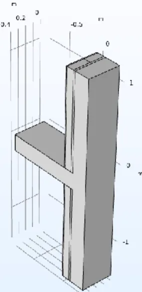
A 3D model (see Figure 3) was created for the thermal bridge assembly as it was suspected that heat transfer would occur through all three planes in the model based on the geometry. The same boundary conditions and material properties were used between the two models, to make a comparison between calculated thermal transmittance values. To ensure enough of the surrounding geometry of the model was analysed, the effective length calculation was performed on the exported heat flux values. A plot was created using the evaluated UX/UO ratio values at each distance evaluated away from the thermal bridge. The plot created a visual showing how the UX/UO ratio decreased and converge to a value of 1 (see Figure 5), finding the effective length to be approximately 0.4 m away from the thermal bridge.
Figure 3: 3D geometry for thermal bridge wall example one The effective length for the example shows that the added heat transfer due to the thermal bridge decrease within the first 0.4 m away from the concrete floor slab, a trend that can be supported by looking at the isothermal planes (see Figure 4). The isothermal planes appear to return to an undisturbed position within the wall assembly beyond 0.4 m, similar to how they appear in the clear field plot (see Figure 2). As the effective length was found within the modeled geometry the overall thermal transmittance (U) value for the assembly with thermal bridge could be calculated 0.63 (W/m2K).
Figure 4: 3D geometric analysis of wall with linear thermal bridge showing isothermal plot
Figure 5: Effective length plot for first example wall Using Equation 2, a linear thermal transmittance value ψ for the concrete slab could be calculated. For the dimensions of the modeled example wall, the calculated ψ value was 0.91 (W/m K), which represents the additional energy lost per unit length caused by an intersecting concrete floor slab through a concrete slab wall.
𝜓 = (𝑈 − 𝑈𝑜) 𝐴𝑟𝑒𝑎 𝐿 Equation 2 U = 0.63 (W/m2 K) UO = 0.28 (W/m2 K) Area = (Height x Length) Height = (1.2 m + 0.2 m + 1.2 m) Length = 0.4 m
As the effective length of this wall assembly was found within the first 0.4 m of the analysed wall, both recommended cut off lengths would have been appropriate to capture the effects of the thermal bridge. To make sure that this trend holds true two other wall assemblies were analysed.
2nd Example Wall
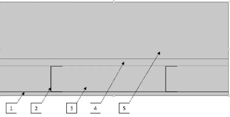
To compare against the first example where the wall assembly did not have any exterior insulation, the wall assembly analysed in this example was an exterior insulated concrete mass wall, with steel studs 16” on center. The exterior insulation was continuous and was rated at 2.64 (m2 K/W). Air was used to insulate the cavity between the steel studs. The geometry for the second wall can be seen below (see Figure 6) with the material properties for this wall are listed in the following table (see Table 2). The thermal bridge in this example was also a concrete floor slab that intersected the steel stud wall.
Figure 6: Clear field geometry for example wall two
Table 2: Material Properties for example wall two # Component Thickness (mm) Conductivity (W/m K) Nominal Resistance (m2 K/W) 1 Gypsum Board 13 0.16 0.08 2 1 5/8” x 1 5/8” Steel Studs 1.02 62 - 3 Air in stud cavity 41 - 0.16 4 Concrete wall/Floor slab 203 1.8 - 5 Insulation Board 100 0.039 2.64 6 Lamina 4 0.9 0.01
Completing the same procedure as in the first example, both a clear wall and thermal bridge model were created for the second wall. Again a conservative 1.2 m was used for the cut-off distance away from the thermal bridge, to ensure the effective length would be captured within the modeled wall.
As adding exterior insulation to a structure is known to be a means of reducing the effects of thermal bridges, it was expected that the thermal resistance of the full wall assembly would not be that different compared to the clear wall performance. For the effective length, it was hypothesised that the exterior insulation used on the thermal bridge wall would result in the whole wall performing almost identically to the clear field wall, and the effective length would be almost negligible. This hypothesis was based on comparing the almost identical thermal transmittance values (see Table 3) from both the clear field wall and the thermal bride wall.
Table 3: Thermal conductivity values for second wall
Assembly
Thermal Conductivity (W/m2 K)
Clear Field (Uo) 0.32 Full Wall with thermal bridge
(U) 0.33
With the addition of the thermal bridge, the thermal resistance of the full wall assembly was only 1% lower compared to the clear wall resistance, which proved that adding external insulation can reduce the amount of energy loss through a concrete slab compared to the wall assembly in example 1 where there was no external insulation. The effective length calculations were performed, with the resulting ratio of UX/UO being plotted (see Figure 7) for the different lengths analysed.
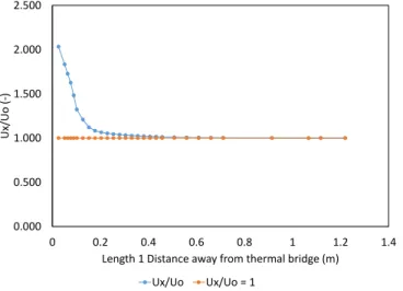
In this example, when length 1 was at its shortest, and most of the wall was being considered, the ratio UX/UO was just greater than 1, (see Figure 7). A UX/UO ratio just greater than 1 shows that, with almost the full wall analysed the overall thermal conductance values is ever so slightly higher than that of the clear wall. When comparing the effective length plot (see Figure 7), to the plot in example one (see Figure 5), it can 0.000 0.500 1.000 1.500 2.000 2.500 0 0.2 0.4 0.6 0.8 1 1.2 1.4 Ux /Uo (-)
Length 1 Distance away from thermal bridge (m) Ux/Uo Ux/Uo = 1
be seen that the UX/UO ratio drop below 1 in example 2, which gives the impression that the wall with the thermal bridge transfers less energy through parts of the wall compared to the clear field wall.
Figure 7: Effective length plot for second example wall When comparing the isothermal plots for the clear wall (see Figure 8) and the thermal bridge wall (see Figure 9), it can be seen that the addition of the concrete slab edge allows more thermal energy to be transmitted through the wall and into the conductive steel studs. The plot of the thermal conductance ratios (see Figure 7) gives a slight misrepresentation of what is going on through the wall in terms of heat transfer as it is only looking at the energy transmitted normal to its surface, and does not capture the energy flowing through the concrete slab, through the base steel studs and into the concrete mass wall. For this example analysing both the isothermal plots and the thermal conductance ratio plot, provide insight into what is happening with the heat transfer through the wall, where the effective length is found at approximately 1 m from the thermal bridge.
Figure 8: 3D geometric analysis of clear field wall showing isothermal plot for second wall
Figure 9: 3D geometric analysis of wall with linear thermal bridge showing isothermal plot for second wall
3rd Example Wall
As a third comparison to the two concrete slab wall an exterior insulated steel stud wall with the studs spaced 16 inches on center was analysed. The cavity space between the steel studs was filled with fiberglass batt insulation. The geometry for the clear wall can be seen below (see Figure 10) with the material properties listed in Table 4. The linear thermal bridge in this example was a concrete floor slab intersecting the steel frame.
Figure 10: Clear field geometry for example wall three Table 4: Material Properties for example wall three
# Component Thickness (mm) Conductivity (W/m K) Nominal Resistance (m2 K/W) 1 Gypsum Board 13 0.16 0.08 2 3 5/8” x 1 5/8” Steel Studs 1.02 62 - 3 Fiberglass batt 92 0.042 2.1 4 Exterior Sheathing 13 0.16 0.08 5 Insulation Board 50 0.039 1.32 6 Lamina 4 0.9 0.01 7 Concrete Slab 203 1.8 -
Following again the same procedure as in the first and second examples, both a clear wall and thermal bridge model were created for the second wall with a conservative 1.2 m used for the cut-off distance away from the thermal bridge.
0.930 0.940 0.950 0.960 0.970 0.980 0.990 1.000 1.010 0 0.2 0.4 0.6 0.8 1 1.2 1.4 Ux/Uo ( -)
Distance away from thermal bridge (m) Ux/Uo Ux/Uo = 1
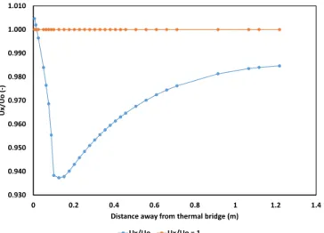
For this example it was speculated that the clear field length would be found to be less than the 1.2 m modeled in the geometry. Figure 11 is a plot of the ratio of UX/UO for this example, which shows how the heat transfer coefficient changes through the wall as the distance away from the thermal bridge increases. In the analysis, when length 1 was at its shortest, the ratio UX/UO was greater than 1. A ratio greater than 1 indicates that for the rate of heat transferred from the area of wall analysed, was greater than that of the clear field wall.
Figure 11: Effective length plot for third example wall The plot shows a point where the ratio value drops below 1 between 0.1 m to 0.7 m. A UX/UO ratio less than 1 indicates that for the section of wall analysed on this plane of reference, there is less thermal energy being transferred from the wall compared to the clear field wall. Looking at the isothermal plots for both the clear field (see Figure 12) and the thermal bridge wall (see Figure 13), it can be seen that, like the second example wall, thermal energy is flowing through the concrete slab. A difference between the second example wall assembly and the wall analysed here is that there is fiberglass insulation between the steel studs. The fiberglass insulation within the stud cavity appears to be limiting the amount of energy transfer being transferred vertically into the steel studs and through the stud wall. When continuing to move further away from the thermal bridge, the thermal conductance ratio approaches and remains around 1 past 0.7 m. The transition back to a ratio of 1 shows that for the area analysed of the thermal bridge wall, the wall is transferring the same amount of energy compared to the clear field wall. When looking at the isothermal plot of the top view of the thermal bridge wall as seen in Figure 14, the isotherms appear almost identical to those shown in the clear field wall Figure 12. This indicates that for this externally insulated wall, the effective length was once again found within 1 m from the thermal bridge.
Figure 12: 2D geometric analysis of clear field wall showing isothermal plot for third wall
Figure 13: 3D geometric analysis of wall with linear thermal bridge showing isothermal plot for third wall
Figure 14: Top view of isothermal plot for third wall
Conclusion
The first conclusion that can be made in this paper is that for all the walls analysed, the recommended cut-off distances from (ASHRAE, 2011) or (ISO 10211, 2017) would be sufficient to capture the effects of the increased heat flow due to the linear thermal bridges analysed in this paper.
0.940 0.960 0.980 1.000 1.020 1.040 1.060 1.080 1.100 0 0.2 0.4 0.6 0.8 1 1.2 Ux/Uo ( -)
Distance away from thermal bridge (m) Ux/Uo Ux/Uo = 1
A second point that should be highlighted is that in all three thermal bridge models, the thermal transmittance was analysed with a cut-off distance of 1.2 m away from the thermal bridge. As the effective length was found within the first 1 m of for all the walls, a cut-off length of 1 m could have been used to model the walls. If for example the thermal bridge model for example one would have been modeled with only 1 m of surrounding wall, the calculated linear thermal transmittance value would been 1.03 (W/m K), a 10 % difference compared to the previous calculated value of 0.91 (W/m K).
This means that for the same thermal bridge, the calculated linear thermal transmittance value is dependent on the simulated geometry as well as the material properties of the assembly. Unless designers trying to quantify the thermal performance of their buildings have ψ and χ values calculated using the exact geometry and materials of their buildings, their calculated values may not represent the true thermal performance of their building. Not having ψ and χ values based on the geometry and materials of the building being analysed, also defeats the purpose of a method intended to reduce computer simulations.
This paper has outlined a procedure that can be used with the help of a simulation tools such as COMSOL, to calculate linear thermal transmittance values for linear thermal bridges found in any project. By outlining a method that shows how linear and point thermal transmittance values can be calculated, building designers can produce their own values based on their specific construction techniques, designs and geometries. With designers being able to calculate their own thermal transmittance values, a better estimation of a buildings performance can be made, helping designers meet the more stringent energy saving targets set out in building codes.
References
1. ASHRAE, ASHRAE Research Project Report - Thermal
performance of building envelope details for mid and high-rise buildings. (2011)
2. ASHRAE, ASHRAE Handbook—Fundamentals. (2017) 3. ASTM, C 1363 Standard Test Method for Thermal
Performance of Building Materials and Envelope Assemblies by Means of a Hot Box Apparatus. (2019)
4. BC Hydro, Building Envelope Thermal Bridging Guide
Version 1.3. Morrison Hershfield Limited. (2019)
5. Ghobadi, M., Moore, T. V., & Lacasse, M. A., Thermal
bridge calculation in the European energy performance of buildings directive. NRC-CNRC, Ottawa (2019)
6. ISO, ISO 10211 - Thermal bridges in building construction
— Heat flows and surface temperatures — Detailed calculations. (2017)
7. ISO, ISO 14683 - Thermal bridges in building construction
— Linear thermal transmittance — Simplified methods and default values. (2017)
8. National Research Council Canada, User’s Guide:
National Energy Code of Canada for Buildings. (2011)
Acknowledgements
The Authors would like to thank NRCan Office of Energy Efficiency for the financial support of the project.