HAL Id: hal-00675583
https://hal.archives-ouvertes.fr/hal-00675583
Submitted on 1 Mar 2012
HAL is a multi-disciplinary open access
archive for the deposit and dissemination of sci-entific research documents, whether they are pub-lished or not. The documents may come from
L’archive ouverte pluridisciplinaire HAL, est destinée au dépôt et à la diffusion de documents scientifiques de niveau recherche, publiés ou non, émanant des établissements d’enseignement et de
To cite this version:
Rosa Meo, Dipankar Bachar, Dino Ienco. LODE: A distance-based classifier built on ensembles of positive and negative observations. Pattern Recognition, Elsevier, 2012, 45 (4), pp.1409-1425. �10.1016/j.patcog.2011.10.015�. �hal-00675583�
LODE: A distance-based classifier built on ensembles of
positive and negative observations
Rosa Meoa,∗, Dipankar Bacharb,a, Dino Iencoc,a
a
Dipartimento di Informatica, Universit`a di Torino, Italy
b
CNRS UMR 7093, l’Observatoire Oc´eanologique de Villefranche sur Mer, France
c
UMR TETIS, Cemagref, Montpellier, France
Abstract
Current work on assembling a set of local patterns such as rules and class association rules into a global model for the prediction of a target usually focuses on the identification of the minimal set of patterns that cover the training data. In this paper we present a different point of view: the model of a class has been built with the purpose to emphasise the typical features of the examples of the class. Typical features are modelled by frequent itemsets extracted from the examples and constitute a new representation space of the examples of the class. Prediction of the target class of test examples occurs by computation of the distance between the vector representing the example in the space of the itemsets of each class and the vectors representing the classes.
It is interesting to observe that in the distance computation the critical contribution to the discrimination between classes is given not only by the itemsets of the class model that match the example but also by itemsets that
do not match the example. These absent features constitute some pieces of
information on the examples that can be considered for the prediction and should not be disregarded. Second, absent features are more abundant in the wrong classes than in the correct ones and their number increases the distance between the example vector and the negative class vectors. Furthermore, since absent features are frequent features in their respective classes, they make the prediction more robust against over-fitting and noise. The usage of
∗Corresponding author
Email addresses: [email protected] (Rosa Meo), [email protected] (Dipankar Bachar), [email protected] (Dino Ienco)
features absent in the test example is a novel issue in classification: existing learners usually tend to select the best local pattern that matches the example - and do not consider the abundance of other patterns that do not match it. We demonstrate the validity of our observations and the effectiveness of LODE, our learner, by means of extensive empirical experiments in which we
compare the prediction accuracy of LODEwith a consistent set of classifiers
of the state of the art. In this paper we also report the methodology that we adopted in order to determine automatically the setting of the learner and of its parameters.
Keywords: Data Mining, Supervised Learning, Concept Learning,
Associative Classifier 1. Introduction
In the last years novel approaches to classification emerged joining two distinct research trends in data mining and machine learning: from one side the rich area of itemsets and class association rules algorithms, which studied in depth efficient algorithms on very large data-sets and on high dimensional data being able to extract large volumes of patterns from data and to enforce on them a rich set of evaluation constraints [1–8]. On the other side the even richer field of machine learning discoveries, whose algorithms and theories were able to combine in powerful classifiers an ensemble of already powerful elementary learners built on a wide spectrum of inductive learning techniques [9–14].
The framework From Local Patterns to Global Models (LEGO) approach
to learning showed how it is possible to join these two worlds trying to com-bine the benefits of the respective fields: manage an increased volume of predictive patterns and at the same time evaluate and assemble them into powerful learners. The resulting model constitutes a general model for learn-ing [15].
Current work [16] on assembling a set of local patterns such as rules and class association rules into a global model for the prediction of a target usually focuses on the identification of the minimal set of patterns that is able to cover the training data. In this paper we present a new learner named
LODE (Learning On Distance between Ensembles) which takes a different
view point. We are convinced that a good model of a class should emphasise the typical features of the examples of the class and that for effective results
!" !" !" !" !" !" !" !" !" !" !" !" !" !" !" !" !" !" !" #$%" &'(" !" )*+" !" !" !" !" !" !" !" !"
Figure 1: Difference between the induction of classification rules by covering and by
pos-sibly overlapping rules, like in LODE
in classification all of them should be used at the same time at prediction time.
In this approach to induction of classification patterns and global model construction we abandon the usual learning strategy based on covering. Cov-ering algorithms often remove the training examples covered by the local patterns already discovered. The removal of examples is motivated by the aim of identifying a global model constituted by a minimal set of as much as possible diverse patterns.
Consider the example shown in Figure 1 in which the examples of the positive class are denoted by the symbol ’+’. By a classical covering al-gorithm, like Ripper [9] and the rule induction systems from propositional learning [17], each new learnt classification rule covers the most numerous set of examples that have not been covered yet by the already learnt rules. Suppose the first classification rule discovered is ABC ⇒ +. After this, all the positive examples matching ABC are discarded from further consider-ations. In Figure 1 these examples are included in the square labelled by
ABC. After the elimination of these examples, another rule like DEF ⇒ +
has no possibility to be extracted because without the discarded examples, it does not cover a sufficiently large set of examples. The unfortunate conse-quence of this covering strategy is that the algorithm misses some rules that have a large support in terms of covered examples and represent a distinctive
set of characteristics of the positive class that would give a more complete characterization to it. As a conclusion, the examples removal by the covering strategy introduces a distortion in the training set which prevents the induc-tion process to learn a sufficient number of characteristics from the removed examples. In practice, it diverts the learning towards the construction of a class model composed of a comprehensive set of characteristics that describes
satisfactorily the examples of a class. Instead, byLODE, all the classification
rules that cover a sufficient number of examples are considered. LODE is
characterized by the following distinguishing issues:
1. the model of each class includes those classification patterns that are frequent w.r.t. the training examples of the class. The frequency con-straint is a guarantee that the pattern has a high coverage and repre-sents recurrent features in the class. Though, we do not require that any two local patterns included in the class model should cover dis-tinct examples. We believe that we should create a global model that emphasises the class characteristics and therefore could contain more patterns that represent the same examples.
2. The selected patterns generate a probabilistic class model that con-sists of a different representation space of the examples. The model of each class is a vector whose components are the selected patterns observed in the training examples of the class. Each vector component is represented with a magnitude equal to the probability with which the corresponding pattern occurs in a random example of the class. 3. We used as classification patterns the frequent set of items (called
item-sets). Itemsets are introduced in Subsection 4.1 [18]. InLODEitemsets
are selected by the innovative criterion of ∆ [19]. ∆ is the departure of the observed frequency of a pattern w.r.t. an estimated frequency of that pattern computed on the basis of the observed frequency of its subsets in the condition of maximum entropy. As a result, a high ∆ occurs in itemsets whose occurrence could not be determined from the observation of their subsets. This fact is an indication that the itemset is not redundant with respect to its subsets in terms of information quantity.
The adoption of ∆ has the aim to control the volume of patterns in the class model. In fact, an increase in the volume of patterns could occur, due to the combinatorial explosion of the items and the combination of unrelated, independent elements into the itemsets.
In a related paper [20] we have validated the use of ∆ for itemsets
selection in classification. As in LODE, in [20] the class models are
based on ensemble of itemsets as well. We have compared ∆ with different alternative measures such as accuracy, KL divergence [21], strong jumping emerging patterns [7]. Experiments showed that ∆ allows to identify the itemsets that make effective the classifiers. 4. Prediction of a test instance occurs by distance computation between
the vectors representing the class models and the projection of the test instance into each class space. In this projection, the role played by the typical characteristics of class examples is crucial: those characteristics that are absent in a test instance but are present in the class model will make the difference between the classes. The predicted class will be the one in which the typical characteristics of the class are absent in the instance as little as possible.
Thus, one of the fundamental differences between our learner and ex-isting prediction techniques based on rules is that our learner uses for the prediction all the patterns of the class model at the same time
-also the patterns that are absent in the test example. Instead, other
pattern-based classifiers, like Class Based Association Rules (CBA), RIPPER, decision lists or decision trees, choose a single rule for the prediction; whereas instance-based classifiers, like k-nn, rely too much on the single examples, that come from local portions of the data-set and could be affected by noise or result in over-fitting.
In the new classifier that we present in this paper, LODE, prediction of
a test instance occurs by distance computation between vectors representing ensembles of local patterns. Our learner is at some extent, similar to ensemble learners, since both combine by an operation of weighed aggregation the contributions of a large number of elementary predictions. Though, ensemble learners like RandomForest or AdaBoost [22] still base the single predictions on patterns which have been recognized present and not absent from the test instance.
We do not compare in this paperLODEwith ensemble learners but only
with elementary classification techniques since our purpose here is to show that our learning technique in itself is already ready to be employed as a
ba-sic learning technique. The local patterns employed inLODE, a combination
both of present and absent patterns from test instances, could still be fur-ther combined into a more sophisticated global model, having performed an
evaluation and aggregation of local patterns typical of boosting or bagging’s combination of elementary classifiers. This is a matter for future work.
The contributions of the paper are the following. We describe and for-malize a new classifier in the context of the LEGO framework. Differently
from many approaches based on local patterns, in LODE the generation of
the class model by local patterns does not occur by a covering strategy but by frequent pattern search. Frequent patterns produce class descriptive models. The class models are vectors composed of the itemsets occurring in the train-ing class examples and are weighed by their probability in the class. By the experimental results of Section 7, we make evident that a descriptive model of the classes, after a suitable simplification and evaluation by a wrapper approach, can be used effectively with a predictive purpose.
The descriptive model is turned into a predictive model by an optimiza-tion, randomized algorithm (Simulated Annealing) whose working points rep-resent the possible cuts in the ranking of the class itemsets. Ranking has been performed by ∆, proposed in our previous works [19, 20]. ∆ is an uncom-mon criterion for the determination of the importance of the itemsets and is related to a non redundancy test between the itemsets and their subsets.
Prediction by local patterns occurs by an ensemble in which all the pat-terns of the class model are used at the same time. Furthermore, prediction makes use not only of the patterns present in the example but also of the ab-sent patterns. We show that the adoption of a multitude of patterns selected from the original class description models makes the prediction more robust against noise and the risk of over-fitting. In this paper we have performed extensive experiments on many data-sets and have conducted a comparison with a consistent set of classifiers of the state of the art. We show that
LODE is specially suitable to the prediction in noisy environments since its
characteristics and its probabilistic nature make it robust against noise. As a conclusion we are able to show its excellent performances.
The last contribution is to show the methodology for the tuning of the
parameters in LODE. Tuning exploits the memory resources of the system
and occurs without the intervention of the user. The contributions of this paper with respect to previous work [20] consist in the formalization of the
overall LODE model, the wrapper approach based on Simulated Annealing,
a more extensive set of experiments that consider both the real and the noisy data and the tuning strategy of the parameters.
This paper is organized as follows. Section 2 provides an overview of
works that combine local patterns into a global model for learning. Section 4 presents the details of the inductive learning technique. Section 5 discusses one of the positive issues of this type of classifier: it has at the same time descriptive and predictive capabilities. Section 6 presents the methodology we adopted in order to automatically set the learner parameters. Section 7 presents the experimental results. Finally Section 8 draws the conclusions. 2. Related work
Associative classification is a popular classification technique which com-bines association mining with classification. CBA [1] is one of the earliest as-sociative classifier which uses association mining to extract association rules from the training data-set. It then ranks the rules based on their confidence. Later it builds a global model from these rules by using a wrapper approach. HPWR [23] is an associative classifier which uses statistical residual analy-sis [24] for the selection of the best associative patterns in the data-set and then uses the weight of evidence [25] in making predictions. IGLUE [26] uses the concept lattice in order to re-describe each instance of the dataset. In the new description of instances the attributes are represented by numerical values according to the number of their occurrences in the concept lattice. It later uses K-nn for prediction. Classifiers based on Emerging Patterns [6–8] choose the associative patterns for each class that are able to discriminate between classes on the basis of their support ratio in different classes. The patterns with larger support ratio are given priority. L3 [27] is another as-sociative classifier which uses a compression method for maintaining more associative rules compared to other associative classifiers. It divides these rule sets into two parts where the first part contains all the specific rules and the second part contains spare rules. During prediction if a matching rule is not found in the first part then the spare rules are used.
Instance based classifiers like K-nn [10, 28, 29] use distance calculation similar to ours. The main difference between our approach and K-nn is that K-nn calculates the distance between each test instance and a (possi-bly large) set of training instances for making prediction. In our approach we calculate the distance between a test instance and a whole global model for each class. Decision tree classifiers like J48 [30] use decision trees where the internal nodes represent tests on attributes and the leaf nodes represent classes. The best matching single path from root to the leaf node is chosen for making any prediction. Rule based classifiers are the closest cousins of
associative classifiers. Typical rule based classifiers like Ripper [30] apply the if − then paradigm for building rules and uses the best rule for any pre-diction. Probabilistic classifiers like Naive Bayes [31] use prior probabilities for calculating all the class conditional probabilities of each attribute. For making a prediction they calculate the posterior probability of the attributes in a test instance. The class with higher posterior probability is chosen as the predicted class. SVM [32] uses the concept of maximum margin hyperplane to find a decision boundary which maximizes the distance between the ex-amples of distinct classes. The decision boundary is the global model which has been built by giving a special relevancy to some local observations in the training set (closest observations coming from different classes). In this sense it is sensitive to the presence of noise in those local portions of the dataset.
Almost all the above mentioned classifiers use local information for mak-ing a prediction, in the sense that they use only those patterns or attributes which are present in both of the test instance and the model constructed
from training instances. Differently, in LODE we use the global information
of a prototypical model of the classes for making any prediction, in the sense that we use all the information contained in each class model as we calculate the distance between each class model and the test instance. According to our knowledge this is a new approach.
Our learner is at some extent, similar to ensemble learners because it combines by an operation of weighted aggregation the contributions of a set of elementary predictions. Though, ensemble learners that make use of bagging, like RandomForest, or boosting, like AdaBoost [22] still base the single predictions on patterns which have been recognized present and not absent from the test instance. Moreover, the basic mechanism by which they learn is different to ours: they generate randomly the basic learners and
during the learning adjust their weights. Instead, inLODEwe generate first a
descriptive model of the class (that acts as a sort of prototype) and learn how to simplify the model by elimination of some of the features. [33] shares the same idea that an ensemble must be composed of millions of patterns but presents important differences w.r.t. our approach: it randomly generates patterns which have a uniform (also low) coverage in terms of the number of examples they match. Patterns are formulated by checking that they do not cover negative examples and are weighted in a uniform way.
s o u r c e d a t a < p , p , p . . . p > 1 1 1 2 1 3 1 d1 < p , p , p . . . p > 2 1 2 2 2 3 2 d2 < p , p , p . . . p > n 1 n 2 n 3 n dn c l a s s n c l a s s 2 c l a s s 1 i t e m s e t r a n k R n i t e m s e t r a n k R2 i t e m s e t r a n k R1 c l a s s 1 c l a s s 2 c l a s s n l o c a l p a t t e r n s f e a t u r e s ( s e l e c t e d p a t t e r n s ) g l o b a l m o d e l 1 2 n M = M = M =
Figure 2: Work-flow ofLODEaccording to theLEGOapproach
3. From Local Patterns To Global Models
LODE is an instantiation of the LEGO approach to classification [15].
LEGO requires an initial extraction of local patterns from the training data,
possibly selected by means of some constraints. Resulting patterns could still be redundant or loosely correlated to the target. Thus local patterns are selected by means of some measure of subsets evaluation. Resulting patterns can be thought as the features on which the classification is based upon. Final patterns are in turn aggregated into an ensemble that constitutes the final global model which is used for prediction of test data.
In Figure 2 we present LODE work-flow according to this approach. In
LODEthe terms (local) patterns and (frequent) itemsets are meant as
inter-changeable. Furthermore, each itemset is a feature in the new representation space of the class examples and each of the features corresponds to a vector component in the class model.
1. From the training examples of source data, frequent itemsets are ex-tracted as the local patterns and separately from each class. Any al-gorithm for frequent itemsets extraction would be valid. The step of frequent itemsets mining can be considered as a black-box from the
possible set of frequent itemsets that main memory allows1. Resulting frequent itemsets generate a lattice. The itemsets with the same cardi-nality are at the nodes of the same level in the lattice and have edges to their subsets and their supersets at the closer lattice levels nodes.
2. Then the itemsets in the lattice of each class Ci are ranked into ranking
Riaccording to some evaluation measure. The purpose of this step is to
raise at the top of the ranking the patterns to be included in the model
of class Ci. In the case ofLODE, as we will see in Section 3.1, the
eval-uation measure is the normalized ∆. Normalized ∆ allows to compare itemsets of different cardinality and, as ∆, allows the identification of which itemsets are not redundant w.r.t. their subsets.
3. The correct top portion of the ranking must be determined so that the ensemble can be simplified, the classifier can be made more robust and efficient and the risk of over-fitting is reduced. As a result of this simplification, each itemset that is in the top portion of the ranking is placed in the ensemble.
4. The ensemble model of the class i is a vector (Mi). Any vector
compo-nent (pij) represents an itemset in the ranking Ri with a weight equal
to its probability (pij) to occur in an example of the class i.
5. The global model is composed of all the class vectors.
The prediction of a test instance is made by projection of the instance in the feature space of each class. The proximity of the projected vector to any class vector is then evaluated for the different classes: the class which is closest to the test instance is predicted.
3.1. ∆ as the Measure to Select the Relevant Itemsets for the
Characteriza-tion of the Classes
We use the criterion of ∆ [19] for the selection of local patterns that will be included in the global model. ∆ is the departure of the observed frequency of a pattern w.r.t. an estimated frequency of that pattern:
∆ = Pobserved− Pestimated (1)
Pobserved and Pestimated are the relative frequencies of a pattern in each
class.
1In the context of our implementation we adopted LCM [34], the winner of FIMI-2004,
The referential estimation is computed in the condition of maximum en-tropy. It represents the frequency that the itemset would have in the case it was maximally difficult to predict its presence when the presence of its subsets was known. In other terms, it is the condition in which the presence of the itemset gives the maximum information when we know the presence of its subsets.
Notice that the estimated probability is a generalized version of the con-dition of independence of the itemset with respect to its subsets: for a pair of items it corresponds to the product of their individual probabilities. For a number of itemsets higher than two there is not a closed formula: the so-lution is found by an iterative, numerical procedure that finds the zero of the derivative of the itemset entropy function [35]. ∆ is a departure from a generalized condition of independence between n items. Thus, it is able to determine a existing dependency between all the items in the n-itemset and to distinguish when a dependency, though present in the itemset, is present because it has been “inherited” by dependencies already existing in the subsets. Summarising, it gives us an indication necessary to distinguish the intrinsic utility of the itemset w.r.t its subsets.
Normalised∆. In this paper we adopted a normalized version of ∆ as follows:
∆ Pobserved
= Pobserved− Pestimated
Pobserved
(2) This normalisation is necessary in order to compare itemsets with different cardinality. In fact, it is well-known that itemsets with a higher cardinality tend to have a lower value of probability. As a consequence, the expected values of ∆ for higher cardinality itemsets are lower.
Itemsets with an absolute value of ∆ close to zero are considered redun-dant w.r.t. their subsets. If two independent subsets are merged to form a new itemset, the contribution of the new itemset to the model would be low because the new itemset does not add new information w.r.t. the subsets. In case of independent subsets, the probability of the supersets corresponds to the estimated probability, obtained in the condition of maximum entropy. Therefore, a ∆ close to zero identifies an itemset that has been formed merely by the combinatorial process of union of items in the itemset formation but do not constitute any specific information, per se. This is an indication that the itemset can be eliminated. Conversely, a high ∆ occurs in an itemset if its subsets are dependent. In that case, the superset would be
interest-ing because identifies related pieces of information that combined appear as non casual. Itemsets that result from the selection based on a high value of normalized ∆ represent the features of interest.
The resulting class model is probabilistic and consists in a characteriza-tion of the class based on frequent itemsets composed by non independent subsets. This is motivated by the need of eliminating irrelevant itemsets from the multitude of frequent itemsets. Indeed, some frequent itemsets, though might occur in the class with a high probability, could be constituted by independent elements; in this case they should not be kept since they do not convey significant additional information for the class with respect to their subsets.
3.2. Selection of the abstraction level
In LODE, ranking is used also to determine unknown characteristics of
the local patterns. The main unknown characteristics of the patterns is the itemset cardinality.
Any lattice level can be considered as an abstraction level at which the class model can be constructed. It is the purpose of the inductive algorithm to learn the correct abstraction level at which the itemsets must be selected in the global model. In fact, itemsets coming from different abstraction levels should not be kept in the model: there would be a duplication of information in the two itemsets when a relationship of specialization (or set containment) exists between them.
InLODEwe used ranking by normalized ∆ also to determine the
abstrac-tion level of the itemsets in the lattice. Ranking the itemsets makes emerge the patterns that are more relevant for the class model. We determined from the top portion of the itemset ranking which are the most recurrent values of the itemset cardinality and produced a rank of the cardinality values denoted
by Rlevels. The best value of the cardinality j will be selected from Rlevels
by a wrapper approach. The wrapper is based on the accuracy obtained by
the classifier LODEwith the class models built on the portion of the itemset
rankings with cardinality j. In particular, the portion Rij of the ranking Ri
is composed of the itemsets extracted from class i with cardinality j. The method is an optimization algorithm based on Simulated Annealing that is responsible also for the ranking reduction (feature selection) and is described in Section 6.5.
4. The Distance-Based Learner on Ensembles of Itemsets In this Section we describe how our distance-based learner works. 4.1. Preliminary definitions
Before entering into the details of the prediction, let us introduce some preliminary definitions. Each test and training example is described by some attributes whose values characterize the instance itself. The values of each attribute belong to a certain domain that could be continuous or discrete. Continuous attribute values are not suitable to be employed in classification by means of class association rules, since they do not often occur frequently in the data. The search for recurrent and frequent itemsets usually works on discrete (categorical or numerical) values in the class examples. Thus contin-uous values are usually discretized in a preprocessing step, by a supervised algorithm like [36].
• Any example in the data-set is represented by a set of attribute-value pairs. We call item an attribute-value pair. For each item a binary variable is associated. For each example of the data-set the binary variable associated to an item has a true value if the example contains that attribute with that value, false otherwise. In this way, the data-set conceptually can be represented as a binary matrix with a row for any example and a column for any item. In each cell of the matrix there is a true or a false value according to the value of the item variable for that example.
• Similarly, from any example we can generate itemsets, as those sets of item variables assuming true values for the example.
• Since we are interested only in recurrent characteristics observed in the examples of a class, we recall only frequent itemsets that occur with a certain, minimum frequency in the examples of the class.
• Let be C = {C1, C2, .., CL} the set of classes.
• Mk denotes the model of the class Ck, with k = 1..L. Mkis represented
as a vector of nk components. Mk constitutes a new feature space of
representation of examples. Each component of the feature space of
class Ck is one of the frequent itemsets extracted from the training
• pki denotes the probability with which i-th itemset (or i-th component)
of the feature space of the class Ck occurs in a random example of class
Ck.
• Mk ≡ hpk1, pk2, ..., pknki
4.2. Projection of a test instance in the class space
Each test instance is described by some attributes whose values char-acterize the instance itself. Similarly, as we represented training instances, by means of itemsets variables with true or false values, we represent test instances, adopting the same representation.
• In order to predict the class of a test instance t it must be represented
in the feature space of each class Ck. This is a projection operation.
• The projection works as follows. We check the presence of each
com-ponent (an itemset) of the class model Mk in the instance t. Let us
denote this generic component as the i-th component. If it is present in t (that is, if every item in the itemset i is present in t), we set the value of the i-th component of t vector to 1; 0 otherwise. In fact, not all the itemsets observed frequently in the objects of a certain class will be present in every test instance, even if the instance comes from that class.
• In the projection we discard those components of t that are not present
in class Ck. In fact, not all the itemsets that are present in the instance
t could be present in a certain class, even if that instance comes from
that class.
As a conclusion, the vector of instance t projected into the feature space
Mk of class Ck is denoted by−→t ⊥−→Mk whose i-th component is:
Ind(i, t) (3)
where the itemset i is the i-th component of the feature space Mkand Ind(i, t)
is the indicator function whose value is 1 if itemset i belongs to test instance t, 0 otherwise.
Vectors are later used for class prediction in a distance computation. Since, class vectors could have a different number of components (features in the feature space) according to the number of frequent itemsets that could
be extracted from the examples of that class, we do not want to favour in the distance computation those classes whose feature spaces have a low number of features since in those spaces data is less sparse and therefore distances result reduced. To solve the problem we normalized the vectors such that their length is 1 and as a consequence distances are not influenced by the number of features in the space. In the following we will use the normalized version of the vectors, indicated by the u operator. The generic i-th component of the normalised vectors is:
u(ti) = Ind(i, t) qP j∈MkInd(j, t) (4) u(Mki) = qPpki j∈Mkp 2 kj (5)
where ti and Mki represent respectively the i-th component of −→t and −→Mk.
4.3. Distance computation between the test vector and the class vectors
The proximity between the two vectors −→Mk and −→t can be computed in
many ways, either as a measure of distance (like the Euclidean distance), or as a measure of similarity (like the cosine similarity), Jaccard or extended Jaccard, etc. Here, we report results obtained by application of the Euclidean distance and the cosine similarity (the results do not differ significantly). No-tice, however, that they have an opposite behavior: the former increases with the dissimilarity of the instance w.r.t. the class, while the latter decreases.
Euclidean distance(−−−−→u(Mk), −−→ u(t)) = s X i∈Mk (u(Mki) − u(ti))2 (6) cosine similarity(−−−−→u(Mk), −−→ u(t)) =−−−−→u(Mk) ∗ −−→ u(t) (7)
Justification of the proximity formulas. It is clear from the formulas 6 and
7 that when a feature (itemset) is present in the class model Mk but it is
absent in the test instance t, its contribution does not increase the value of cosine similarity and increases the Euclidean distance. On the other side, when the total number of features in the class is high, the contribution to
each of them is lower (because of the normalisation factor). However, in this normalisation factor even absent features have their weight and contribute to decrease the weight of all the other features (also the present ones). 4.4. Formalization of the problem with an objective function
LODEframework can be formalized as a problem of learning the
compo-sition of the class models in terms of the frequent itemses extracted from the training examples. The learning makes use of an objective function 8 that guides the tuning of the models and can be formalized as follows.
Let C = {C1, C2, .., CL} be the set of classes and Tr = ∪Li=1Trithe training
set where Tri is the subset of the examples of class Ci. The goal of the
learning task is to find the set of class models {M1, M2, .., ML} in which each
Mi is composed of frequent itemsets occurring in the examples of Tri. Each
itemset j describes a set of characteristics occurring in the examples of Tri
with frequency pij. Each Mi maximizes an objective function:
X t∈Tri
Ind{proximity(−−−→u(Mi),−−−−−−−u(t ⊥ M→i)) > proximity(−−−−→u(Mj),−−−−−−−→u(t ⊥ Mj))}, with j 6= i (8) where the proximity function is equation (6) or equation (7), t is an example
of class Ci in the training set Tri. The unary indicator function Ind{·} is 1
if its parameter is true, 0 otherwise. The parameter: proximity(−−−→u(Mi), −−−−−−→ u(t ⊥ Mi)) > proximity( −−−→ u(Mj), −−−−−−→ u(t ⊥ Mj)
is the condition for the true class prediction. The proximity is computed between two vectors: the unit vector representing the class model and the unit vector representing a single training instance projected in the class space.
The objective function increases for the class model Mi when the proximity
between the class model vector and the training instance vector is higher
then for the other class models Mj. In other terms, the objective function
represents the number of correct predictions for class Ci.
The tuning step of LODE for the determination of the composition of
Mi selects the itemsets from a ranking Ri. The itemsets in Ri have been
ranked by an evaluation measure (that in our case is the normalised ∆). Let
denote by Ril the set of itemsets in Ri of cardinality l. The selection of the
itemsets in Mi is made by determination of the itemset cardinality value l
(abstraction level) and of a cut of the ranking Ril, such that the top portion
of the ranking is retained in Mi and the portion below the cut is discarded.
The cut has been formalised by the determination of a percentage ri of the
4.5. LODE on a toy example
In Figure 3 we show a toy sample from the Play Tennis data-set, a well-known example of a prediction problem of the suitable weather conditions for playing tennis. From the examples of the two classes (Yes and No) separately,
LODEextracts the frequent itemsets. The two diamonds represent the
item-sets search space that has the form of a lattice. LODE ranks the itemsets
according to the value of the normalized ∆ (NDelta). Then, the itemsets cardinality equal to a value of three is selected (see the method described in Subsection 3.2). For each itemset, the value of the relative frequency in the class is reported. In the picture, due to lack of space, only the first six itemsets are shown in the ranking, out of the total of eleven extracted item-sets. These ensembles constitute a descriptive representation of the classes in which the order of the features is informative of its importance in the description.
In Figure 4 we show instead the test phase of LODE. On the left, the
vector model of class Yes is composed by the eleven itemsets that were in the corresponding ensemble. Each itemset is represented in the vector by its relative frequency in class Yes. Analogously for the other class whose vector is shown on the right. Below, we show both the vector models with numerical values, after normalization.
In the center of the picture a test example is taken. At the bottom, the picture reports the vectors representing the test example under the viewpoint of the classes. They have been obtained by means of projection of the origi-nal test vector in the feature space of each class and normalized. Fiorigi-nally, the distance between the unit test projected vector and the class vector is com-puted. In this example, class No is predicted. In fact, class Yes has only one present feature (which in addition occurs in the class with a low frequency) while class No has four features (and the first one is very frequent). In this example, both the number and the frequency of the present features make the difference in the computation of the two distances which depend also on the number of absent features in the test vector projected in the class space.
5. Descriptive and predictive capabilities of LODE
The distinctive issue inLODE is the adoption of a descriptive model for
a final predictive goal. The question that we want to answer with this work is: does a descriptive model support a predictive task? We will ask with the empirical evidence of the extensive experiments performed at Section 7.
Frequent itemsets (minsup=33%)
Triplets in class P=Yes ranked by Normalized Delta
O=Rain, T=Mild,W=Weak NDelta=... pYes1=0.66 T=Mild, H=High, W=Weak NDelta=... pYes2=0.33 O=Rain, H=High, W=Weak NDelta=... pYes3=0.33 O=Rain, H=High, W=Mild NDelta=... pYes4=0.33 T=Hot, H=High, W=Weak NDelta=... pYes5=0.33 O=Sunny, T=Hot, H=High NDelta=... pYes6=0.33
Triplets in class P=No ranked by Normalized Delta
O=Rain, H=Normal, W=Strong NDelta=... pNo1=0.66 O=Rain, T=Cool, W=Strong NDelta=... pNo2=0.33 T=Cool, H=Normal, W=Strong NDelta=... pNo3=0.33 O=Rain, T=Cool, H=Normal NDelta=... pNo4=0.33 O=Sunny, T=Hot, W=Strong NDelta=... pNo5=0.33 O=Sunny, T=Hot, H=High NDelta=... pNo6=0.33 Play Tennis dataset
OutLook (O) Tempe-rature (T) Humidity (H) Wind (W) Play Tennis (P)
Rain Mild Normal Weak Yes
Sunny Hot High Weak Yes
Rain Mild High Weak Yes
Rain Cool Normal Strong No
Sunny Hot High Strong No
Rain Mild Normal Strong No
Figure 3: Example on Play tennis data-set byLODE
The benefit is that it is possible to obtain both a descriptive model of the classes and a predictive model, at the same time. Furthermore, the test instance vector projected onto the class models constitutes a descriptive representation of the test instance itself. This model is interpretable: it is composed by an ensemble of itemsets where each itemset is in practice
Vector Model MYes for class P=Yes
< pYes1, pYes2, ... pYes11>
< pNo1, pNo2, ... pNo11>
Vector Model MNo for class P=No
< pYes1/||MYes||, ... , pYes11/||MYes|| >
Unit vector U[MYes] for class P=Yes
< 0.53, 0.26, 0.26, 0.26, 0.26, 0.26, 0.26, 0.26, 0.26, 0.26, 0.26>
<pNo1/||MNo||, ..., pNo11/||MNo|| >
Unit vector U[MNo] for class P=No
< 0.53, 0.26, 0.26, 0.26, 0.26, 0.26, 0.26, 0.26, 0.26, 0.26, 0.26> test example t1: OutLook (O) Tempe-rature (T) Humidity (H) Wind (W) Play Tennis (P)
Rain Mild Normal Strong No d(U[t1!MYes], U[MYes])=
1.199
d(U[t1!MNo], U[MNo])= 0.647
< 0, 0, 0, 0, 0, 0, 0, 0, 1, 0, 0> test example t1 projected in
class Yes feature space (unit vector): U[t1!MYes]
<0.5, 0, 0, 0, 0, 0, 0, 0, 0.5, 0.5, 0.5>
test example t1 projected in
class No feature space (unit vector): U[t1!MNo]
Figure 4: Test example on Play tennis data-set by LODE
a sentence composed by a conjunction of predicates that are true for the instance and are frequent in the class. Furthermore, each predicate sentence is equipped with a weight equal to the probability of its occurrence in the class examples. This weight is then reduced by the total number of sentences (if many sentences are applicable each of them weighs less).
The number of class features that apply to the test instance tells us how much that instance is similar to the class. Finally, the evaluation measure of the proximity between the test vector and the class vector quantifies the similarity between the test instance and the class.
concept, unfortunately rarely adopted in data mining - it is possible to dis-tinguish which of the itemsets are really relevant to determine a complete, but non redundant, set of characteristics describing a class of examples.
Certainly related to this concept are the concepts of miki, maximally informative k-itemsets [37] and pattern teams [38]. Both make use of the concept of maximum entropy but they do not make use of the departure with respect to it. Indeed, their aim is orthogonal to ours. Miki’s aim is to identify the minimal set of items that is able to distinguish between the examples in the data and search for the set of items that are distributed in the most uniform way in the data-set. Similarly pattern teams’ aim is to select from a set of local patterns the minimal set that is non redundant and that allows a maximal covering in terms of the number of the examples they represent. Instead, our aim is descriptive: in the class model we want to identify the most complete set of patterns that catch all the class features observed in the training set. This ensemble of patterns collectively provides a probabilistic description of the class. It is composed of itemsets that have a good coverage each (because each of them is frequent) and such that each of them is not redundant.
Related to our goal is the field of subgroup discovery [39, 40]. In subgroup discovery, the set of patterns selected for the representation of a subgroup of the population does not need to provide a complete description of the target but needs to represent a set of interesting characteristics. The difference of our approach w.r.t. subgroup discovery is that our model aims to provide a complete description of the class while subgroup discovery accepts to describe only a portion of the target but it achieves a statistically sound description of a subgroup of examples. It would be possible to adopt a subgroup discovery model and adapt it to a predictive goal by means of the distance-based ap-proach on positive and negative descriptions as described in this paper. This will be the theme of a future research work. Currently, the authors of [40] make the reverse: they adapt a rule induction algorithm with a predictive goal to the subgroup discovery task.
On itemset redundancy. Itemsets redundancy is tested in our model by ∆
with respect to the itemsets subsets and not with respect to their peer-itemsets. This operation by ∆ is simpler than other standard statistical
methods like the test of independence by χ2 or on correlation by Pearson
coefficient. Both these tests work on pairs of patterns. Instead, ∆ does not involve the peer-itemsets but their subsets (whose number is much lower than
0 20 40 60 80 100 Percentage of redundant itemsets with cardinality=2 Percentage of redundant itemsets with cardinality=3 !"#$"%&'(") *'&'+"&)
Figure 5: Percentages of redundant itemsets by Chi-square at different cardinality levels.
the number of peer-itemsets). Furthermore, the results of the experiment we are describing in the following do not justify the search of redundancies be-tween the peer-itemsets. We checked the number of dependent peer-itemsets
by χ2 test. The test is done at different cardinality levels of the itemsets. In
Figure 5 we report the percentages of redundant itemsets at the cardinality
level 2 and 3 detected by χ2 in a few UCI data-sets. We observe that the
percentage of redundant itemsets reduces dramatically as soon as the item-sets cardinality increases. This is due to the following fact: as a consequence of the construction of itemsets, the space gets more sparse and the number of redundancies between itemsets results reduced.
In agreement to these observations, many algorithms of rule learning try to reduce redundancies between the rules. Very often they work on redun-dancies between the original features (in our case, the items). One example is [41] which learns class association rules by an Apriori-style algorithm [18]. During rule generation Apriori-C checks that for each rule there is not al-ready one of its generalisations that has a better coverage. This test aims to reduce the number of rules and is based (as ∆) on the comparison between an itemset and its subsets. Rules are ordered according to their quality measure
but, in contrast to LODE, one single rule is applied to each test example.
6. Methodology of Learner Setting
In this Section we present the methodology we adopted to generate the local patterns, and later tune the model: select a subset of the local patterns for the creation of a global model.
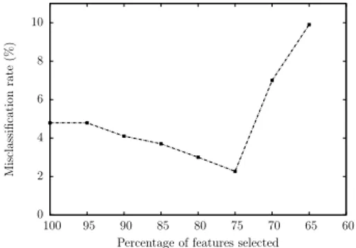
6.1. Motivations for the ensemble reduction
In Figure 6 we present a study on the effect of the dimension of the ranking
of local patterns Rkon the misclassification rate. As we explained, we ranked
the local patterns by the evaluation measure (normalized ∆). We reduced the dimension of the class models by elimination of the bottom part of the rankings. Figure 6 shows an initial gradual improvement of the classification accuracy which is due to a simplification of the models that leads to a better generalization capability and a reduction of over-fitting. After the optimum point, the model worsens because too many itemsets have been eliminated from the model and the error rate starts to increase.
0 2 4 6 8 10 60 65 70 75 80 85 90 95 100 M is cla ss ifi ca tio n ra te (% )
Percentage of features selected
Figure 6: Error rate on Wisconsin-Breast-cancer with class models built on different number of itemsets 0 2 4 6 8 10 12 14 16 0 0.05 0.1 0.15 0.2 M is cla ss ifi ca tio n ra te (% )
Minimum support threshold
Figure 7: Misclassification on
Wisconsin-Breast-cancer by class models on frequent itemsets at different minimum support
6.2. Effect of the minimum support threshold on classification
In Figure 7 we observe the relationship between the minimum support threshold that governs the algorithms of frequent itemsets mining and the misclassification rate of the ensemble of local patterns. We notice an im-provement in classification accuracy by decreasing the support threshold. This tells us that even itemsets with a not very high frequency could be useful for the classification since their normalized ∆ value could be high. 6.3. Determination of the value of minimum support threshold
How many itemsets do we have to collect? We believe that we could try to collect the highest possible number of itemsets that our computing system can allow: it will be responsibility of the normalized ∆ their final selection in the global model. Thus in Figure 8 we plot the total number of itemsets
0 500 1000 1500 2000 2500 N u mb er of i te ms ets Support values Real itemsets Estimated Itemsets
Figure 8: Histogram on the number of itemsets in class malignant of Breast.
having a frequency in the interval indicated at the x axis. Knowing this histogram we can decide a suitable value of the minsup parameter (i.e., the minimum itemsets frequency allowed) given the total amount of memory in our system: it is sufficient to sum up the total number of itemsets taken from the histogram starting from the highest support value and going towards the left until the maximum memory size is reached or the support reached is 0. (In other words we consider the histogram as a probability density function of the itemsets, and compute the area under it from the right).
The construction of the exact histogram is of high computational cost if it is constructed by running an algorithm of frequent itemset mining on a large data-set. Thus we suggest the following strategy.
1. We simply count the frequency of singletons (items) in the data. 2. We compute the frequency of other itemsets under the hypothesis of
statistical independence of items and generate the histogram of the number of itemsets with a frequency equal to a certain value determined by the interval indicated at x axis (see Figure 8). You can notice that the real and the estimated histograms differ only at low frequency thresholds.
3. We select the support threshold directly on the estimated histogram and this choice is conservative.
If we wished to establish instead the correct number of itemsets at lower support values, we could collect a sample of the data and test in the sample the total number of itemsets without the hypothesis of statistical independence. In Figure 9 we show that this approach is
practical since the total number of itemsets collected does not differ significantly with the dimension of the sample (the percentages of the sampled examples are indicated at the x axis). Thus this strategy is computationally feasible, since it requires to collect only a little portion of the data-set. In this initial sample we lower the minimum support threshold and observe the total number of itemsets extracted. The right threshold is the one that gives the maximum number of itemsets that the system memory allows.
0 500 1000 1500 2000 2500 10 20 30 40 50 60 70 80 90 100 N u m b er of it em se ts
Percentage of sampled dataset
Figure 9: Total number of itemsets from Breast data-set with progressive sampling
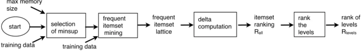
6.4. Initialisation of LODE
Figure 10 shows the diagram of the initialization ofLODE. After the first
step of determination of minimum support threshold (according to the algo-rithm described in Section 6.3) the algoalgo-rithm of frequent itemsets mining is launched on the training-set and produces a set of frequent itemsets that are
ranked according to their normalized ∆ value (ranking Rall). This initial,
unique ranking tells us some things regarding some unknown but charac-teristic parameters of the itemsets, as already explained in Subsection 3.2. First of all the most recurrent value of cardinality of the itemsets at the top portion of the ranking (top portion is set to 2/3). The most recurrent value of itemsets cardinality at the top of the ranking is the first value that will
be tested in the following tuning process ofLODEin order to select itemsets
for the class models (see Section 6.5). Then, the other cardinality levels are
start selection of minsup training data max memory size frequent itemset mining frequent itemset lattice delta computation training data itemset ranking Rall rank of levels Rlevels rank the levels
Figure 10: Initialisation of parameters and of tuning ofLODE
of the itemsets at the top portion of the ranking Rall. This is done because it
is necessary to determine a unique value of cardinality for the itemsets in the class models. Indeed, it makes no sense to include itemsets with a different cardinality value as components of the class vectors since some dependencies exist between itemsets and their subsets.
6.5. Tuning step of LODE
The pseudo-code of the algorithm that performs the tuning process of the class models is Algorithm 1. This tuning process has been performed in all the experiments that will be described in Section 7 within a 10-fold cross-validation (from line 6 to 37): we repeated this process 10 times on different training sets and with a different validation set and test set. For each training set there is a separate validation set. On each training set the learning algorithm produces a model (lines 14-19) with parameters which are optimised by the tuning algorithm on the validation set (lines 22-33). As can be observed from Algorithm 1, since the discretization performed by Fayyad and Irani’s method [36] is a supervised step, we have to guarantee that no information on the class outcomes towards the test sets in an hidden way through the information on the discretization. Thus, the discretization has been applied ten times as a pre-processing step to each different training-set (see lines 10-11) and re-applied ten times to the corresponding test set (line 34). Each test-set is then used to evaluate the classification accuracy of the generated models (lines 35-36) and gives in output the average of the values of misclassification for the ten test folds (line 38).
1. At lines 7-11 the cross-validation procedure is prepared; discretization is applied as a pre-processing step to each different training-set of the cross-validation loop.
Algorithm 1 Feature Reduction Tuning Process of LODE within Cross-Validation
1: Input: D data-set 2: Input: MaxMemorySize
3: Output: TotErr LODE classification error
4: set small and big perturbation (percentage reduction) in rankings -5: s = 0.0002, b = 0.05, TotErr = 0, Nfolds = 10
6: for testFolds = 1 to Nfolds 10folds crossvalidation
-7: divide D into disjoint portions: training-set Tr, validation-set V, test-set T
8: apply Fayyad Irani supervised discretization on trainingset and validationset
-9: set of attribute value intervals S = FindSupDiscr(Tr ∪ V)
10: discTr= applyDiscretization(Tr, S)
11: discV = applyDiscretization(V, S)
12: - - Initialisation of minsup and ranking of cardinality levels by Algo. in Fig. 9
13: initialise(discTr, MaxMemorySize, minsup, Rlevels)
14: - - extract itemsets from discretised training-set and rank them by Norm. Delta
15: Rall =generate-itemsets-and-rankings(discTr, minsup)
16: - - Rij is the portion of Rall with freq. itemsets at cardinality j for class i
17: iteration it = 1
18: l = first cardinality level from Rlevels
19: OptimalRi = Ril initialisation step
-20: BestErr = HIGHEST ERR VALUE - - initialise with worst possible error
21: stop = FALSE
22: repeat
23: Tune class models by Simulated Annealing on LODE classification error
-24: CurrentErr = SA (discV, Ril, s, b) - - call Algo. 2
25: ∆Err = BestError-CurrentErr
26: IF (∆Err < 0)
27: BestErr = CurrentErr
28: OptimalRi= Ril
29: END IF
30: IF (e(∆Err)/it ≤ rand(0, 1)) stop = TRUE
31: it++
32: l = next cardinality level in Rlevels
33: until stop
34: discT = applyDiscretization(T, S)
35: errorOnTestFold = LODE(discT,OptimalRi)
36: TotErr = TotErr + errorOnTestFold
37: end for
38: return TotErr/Nfolds
2. At line 13 the initialization phase determines the minimum support value (by algorithm described at Figure 10) and generates the rank of
itemsets cardinality levels (Rlevels).
3. At the lines 16-20, during the first iteration (it=1), the sets of frequent itemsets are extracted separately from the classes of the training set (with the same minimum support proposed by the initialisation step);
the itemsets for class i are ranked in ranking Ri. They are given in
input to the phase of itemset cardinality selection (lines 22-33) for the construction of the class vectors. The level is taken from the rank of levels (Rlevels) obtained at initialisation.
4. From the collections of itemsets at the selected level of cardinality l
separate rankings are obtained for the various classes (Ril). We denote
by Ril the different portions of the ranking Ri, where l represents the
cardinality level of the itemsets.
5. This is the phase of feature reduction on the rankings Ril (at line 24).
Since from Figure 6 we saw that the feature selection on the rankings (ranking reduction from the bottom) is beneficial for classification, but we do not know how many minima of the classification error are present, we adopt an algorithm of global optimization (Simulated Annealing, SA) in order to search for the optimum reduction. The pseudo-code of the algorithm of SA is shown in Algorithm 2. We note that SA is executed on the validation set on the rankings obtained on the training set.
6. After SA algorithm stops, a minimum of classification error is obtained in correspondence to the rankings of itemsets at the cardinality level l. Delta error (∆Err) is obtained w.r.t. the best error obtained at previous iterations (which worked on rankings of itemsets with a dif-ferent value of cardinality l). Stop condition (line 33) is probabilistic.
It is set to true when e(∆Err/it) <= rand(0, 1). It is similar to the
condition seen for entering into a big perturbation in SA: it depends on the reduction in error computed in the current iteration w.r.t. the best error obtained so far, the number of iterations already computed and by a random value. According to this exponential formula, stop is encouraged if the number of iterations is high and if the error is not improving (∆Err is negative).
The approach to feature selection operated by SA in Algorithm 2 is a wrapper approach. The rankings are progressively reduced and the decrease
in classification error on validation data by the classification algorithmLODE
local minimum (line 12 of Algorithm 2) small perturbations are sufficient (small ranking reduction). Otherwise, if we need to escape from a local minimum (line 17), in order to find a global minimum in the error, we have the chance to escape if we adopt a big perturbation (percent big reduction of the rankings). In the experiments we set the big reduction to 5% while the small reduction consists in 0.0002 (corresponding to a single itemset with a ranking of 5 thousands itemsets). Our implementation of SA has been adjusted by us to the particular contest: the direction of movement on the ranking is unique (bottom-up) when a small reduction is involved. Instead, when a big reduction takes place, it searches the closer minimum in both the directions (top-down and bottom-up).
The condition for the adoption of a big perturbation is again probabilis-tic: it is governed by a random function (rand), decreases with the number of iterations computed (parameter I) and increases with the obtained im-provement in the error (∆Err).
Algorithm 2 Itemsets Selection Algorithm by Simulated Annealing
1: Input: V validation-set
2: Input: Ri ranking of frequent itemsets.
3: Input: s small ranking reduction (perturbation) 4: Input: b big ranking reduction (perturbation)
5: Output: Optimal reduction of Ri based on classification error.
6: – Tune class models by calling LODE algorithm –
7: InitialError = LODE (V, Ri ) 8: CurrentError = InitialError 9: MinError = InitialError 10: I = 1 11: repeat 12: perturb (Ri, s) 13: CurrentError = LODE(V, Ri)
14: ∆Error = CurrentError - MinError
15: IF ( ∆Error < 0) 16: MinError = CurrentError 17: OptimalRi = Ri 18: ELSE IF ( ∆Error >= 0 ) 19: IF (e(∆Error)/I > rand(0, 1)) 20: perturb (Ri, b) 21: I++
22: until I > upper limit of I 23: return MinError
7. Experimental Results
We have implemented LODE in C++. ∆ computation and ranking
gen-eration is instead in java. We implemented some scripts in python and perl for the automatising of the whole procedure. In future work we are going to implement all the modules in a unique programming language and equip the system with a web-based graphical user interface. Current version of the software can be down-loaded from:
http : //www.di.unito.it/emeo/Algo/LODE.zip.
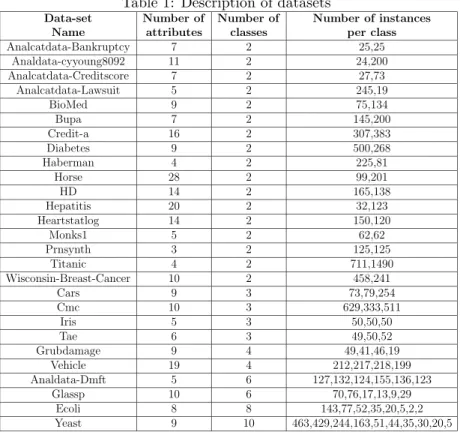
We have performed classification experiments withLODEon several datasets
from the Machine Learning Repository, maintained by UCI as a service to the machine learning community (http://archive.ics.uci.edu/ml/). Table 1 reports the various characteristics of the datasets, chosen for their wide vari-ability in terms of the type of data, number of classes, number of examples, number of attributes, total number of instances per class (indicated in table separated by commas), availability in competitive algorithms, etc. Experi-ments were run on a Pentium Intel core Duo processor (P9500), running at 2.53Ghz with a RAM of 1.95 GB.
We compared the classification performances of our classifier with many well known classification algorithms: Knn [10], J48 [30] (an implementa-tion of Decision Trees), Naive Bayes [42], Support Vector Machines [43] and decision table [44], CBA [1] and RIPPER [9] as representative learners for conjunctive rules-based classifiers. We included also L3 [27] as a representa-tive learner from the set of classifiers that learn by a multitude of rules. We used the implemented version of these classifiers that is available in Weka (http://www.cs.waikato.ac.nz/ml/weka/), a collection of machine learning algorithms for data mining tasks.
Notice that some datasets contain only categorical attributes, while others contain also continuous ones. Itemsets are usually extracted from categorical attributes: in fact, from continuous attributes itemsets would have hardly a
sufficient frequency. In order to be able to run experiments with LODE and
the associative classifiers, we performed a preprocessing step consisting in a supervised discretization of continuous attributes by means of a method based on entropy [36] that minimizes the entropy of the class given the inter-val of discretization. We used a unique data-set discretization method (by Fayyad and Irani) for all the classifiers that require a discretized data-set and that do not perform discretization by themselves. Instead, for those methods that have their own discretization embedded in the learning algorithm (like
Table 1: Description of datasets
Data-set Number of Number of Number of instances
Name attributes classes per class
Analcatdata-Bankruptcy 7 2 25,25 Analdata-cyyoung8092 11 2 24,200 Analcatdata-Creditscore 7 2 27,73 Analcatdata-Lawsuit 5 2 245,19 BioMed 9 2 75,134 Bupa 7 2 145,200 Credit-a 16 2 307,383 Diabetes 9 2 500,268 Haberman 4 2 225,81 Horse 28 2 99,201 HD 14 2 165,138 Hepatitis 20 2 32,123 Heartstatlog 14 2 150,120 Monks1 5 2 62,62 Prnsynth 3 2 125,125 Titanic 4 2 711,1490 Wisconsin-Breast-Cancer 10 2 458,241 Cars 9 3 73,79,254 Cmc 10 3 629,333,511 Iris 5 3 50,50,50 Tae 6 3 49,50,52 Grubdamage 9 4 49,41,46,19 Vehicle 19 4 212,217,218,199 Analdata-Dmft 5 6 127,132,124,155,136,123 Glassp 10 6 70,76,17,13,9,29 Ecoli 8 8 143,77,52,35,20,5,2,2 Yeast 9 10 463,429,244,163,51,44,35,30,20,5
decision trees) or that do not require a discretized data-set (like K-nn, SVM, etc) we let them the original data-set.
We did discretization and parameters tuning within a 10-fold cross-vali-dation. The division in folds is the same for all the learning algorithms. We performed cross-validation with (disjoint) training set, validation set and test set. Validation-set and test-set are folds from the 10-fold-cross-validation. Training set instead is made by the remaining part of the data-set. We never used the test folds for parameter tuning or discretization: we used test folds only for accuracy testing of the algorithms. For each training-set in the cross-validation, we performed learning of the model and used the validation set to estimate the suitability of the parameters values.
We carefully tuned the parameters values of the competitors as Figure 2 shows. We tested all the combinations of values of their parameters taken from a wide spectrum of possible values with the reported variation step.
Table 2: Parameters and their range of values used in the tuning process of learning competitors
learner parameter range of values step
J48 pruning confidence 0.05 – 0.5 0.05
J48 instances per leaf 2 – 10 1
DTABLE n. folds cross-valid. 1 – 10 1
DTABLE perf. eval. measure [acc,rmse,mae,auc] 1
NB no parameters needed – –
SVM (SMO) complexity C -3 – 3 0.25
SVM (SMO) polyKernel exp. 1 – 3 0.5
RIPPER n. folds for REP 1 – 10 1
(1-fold as pruning set)
RIPPER min inst. weight in split 0.5 – 5 0.5
RIPPER n. optimiz. runs 1 – 10 1
KNN k 1 – 10 1
CBA minsup 1% –
CBA minconf 50% –
of the optimal parameter values that we obtained by the parameter tuning
process of LODE. In particular, for LODE, we applied the tuning process
described by Algorithm 1.
The overall results of our experiments in comparison with other classifiers are presented in the series of tables Figure 11-Figure 5. Each Figure shows
the results obtained for the comparison of LODEwith the other competitors
on many viewpoints: classification accuracy, training time, test time. In order to compare the statistical significance of the observed difference we adopted the approach overviewed in [45]. It presents the statistical test proposed by Friedman on average rankings applied to classifiers performance results. We briefly summarize the test here.
1. The performance of each classifier on a certain issue (accuracy, training times, etc) is determined on each data-set.
2. The classifiers are ranked on each data-set according to the results. 3. For each classifier, its position in the various rankings is recorded and its
average position w.r.t. the data-sets is computed. This is the resulting value that we give in output in the tables. The advantage is that it allows to present a comparison of multiple classifiers on multiple data-sets.
4. The observed differences between the average rankings are compared with the critical difference CD which establishes whether the differences
are statistically significant: CD = qα
q k(k+1)
6N where N is the number of
datasets, k is the total number of classifiers, α is the significance level
and qα is the critical value for (k−1)α based on the Studentized range
Table 3: Optimal parameters values resulting from tuning process inLODE
Percentage of Standard
Data-set Cardinality Minimum features retained deviation of
name level support (mean of ten folds) retained features
threshold (ten folds)
Analcatdata-Bankruptcy 3 0.01 100 0 Analdata-cyyoung8092 3 0.05 89.36 1.7 Analcatdata-Creditscore 4 0.01 100 0 Analcatdata-Lawsuit 3 0.01 100 0 German 4 0.3 75.37 2.36 BioMed 5 0.01 76.89 3.7 Bupa 3 0.05 87.47 1.73 Australia 3 0.3 84.3 1.9 Labor 4 0.1 96.9 1.13 Sonar 4 0.3 73.23 6.7 Wave 4 0.2 70.39 2.33 Lymph 4 0.3 89.9 7.81 Diabetes 3 0.05 78.37 1.3 Haberman 2 0.01 93.13 2.37 Horse 2 0.15 90.71 1.29 HD 3 0.2 86.43 5.18 Hepatitis 4 0.2 89.5 1.3 Heartstatlog 3 0.1 81.13 3.39 Monks1 5 0.01 85.16 4.33 Prnsynth 2 0.01 87.31 1.36 Titanic 2 0.01 85.3 2.19 Wisconsin-Breast-Cancer 4 0.01 92.27 1.39 Cars 5 0.01 93.14 2.79 Cmc 4 0.05 90.12 1.36 Iris 4 0.05 97.1 1.7 Tae 2 0.05 94.13 3.69 Grubdamage 4 0.05 95.1 4.1 Vehicle 4 0.2 93.24 1.3 Analdata-Dmft 3 0.1 97.4 1.2 Glassp 3 0.01 91.39 2.1 Ecoli 5 0.05 96.27 1.7 Yeast 3 0.1 98.1 1.3
In our tests we used the value of α equal to 0.05 and the corresponding
value of qα equal to 2.394.
The first important observation that comes out from the Table in
Fig-ure 11 is that LODE outperforms the other learners as regards the
classi-fication accuracy (on test set, with 10-folds cross-validation). LODE mean
ranking is equal to 1.46875 and since the second ranked classifier is SMO with a mean rank of 4.15625 and the value of CD is equal to 1.864995 the observed differences are statistically significant. The graphical representation of the Friedman test on the differences in classification accuracy is presented in Figure 12.
Classifier Name Mean Rank
threshold (CD) 1.864995 LODE 1.46875 SMO 4.15625 CBA 4.203125 KNN 5.03125 NB 5.515625 J48 5.578125 L3 6.078125 RIPPER 6.171875 DTABLE 6.796875
Figure 11: Mean ranking on clas-sification accuracy of classifiers on original datasets (test set)
1 2 3 4 5 6 7 8 CD LODE SVM CBA KNN NB J48 L3 Ripper Dtable
Figure 12: Graphical representation of Friedman test on differences in classification accuracy
In Figure 13 we show the analogous statistical test on the difference be-tween the accuracy on training-set and the accuracy on test-set. This ex-periment aims at putting in evidence the capability of a classifier to escape
from over-fitting. We can see that NB is ranked first, CBA second and LODE
third but these differences are not statistically significant.
In Table 4 we report the details of the classification error (and of the
difference between the error on the training-set and on the test-set) of LODE
and of SMO, which is among the learners the one whose performance gets
closer to LODE. We reported also the details regarding the kind of datasets
(number of classes, balanced classes, number of features) in order to ascertain if the obtained good results could be also related to the typology of data or not. From the results it is clear that good results could be obtained both in binary and in multi-class data, balanced or unbalanced, high-dimensional or not.