Computer Science and Artificial Intelligence Laboratory
Technical Report
m a s s a c h u s e t t s i n s t i t u t e o f t e c h n o l o g y, c a m b r i d g e , m a 0 213 9 u s a — w w w. c s a i l . m i t . e d u
MIT-CSAIL-TR-2014-018
September 2, 2014
Alloy*: A Higher-Order Relational
Constraint Solver
Aleksandar Milicevic, Joseph P. Near, Eunsuk
Kang, and Daniel Jackson
Alloy*: A Higher-Order Relational Constraint Solver
Aleksandar Milicevic
Joseph P. Near
Eunsuk Kang
Daniel Jackson
Massachusetts Institute of Technology Cambridge, MA, USA
{aleks,jnear,eskang,dnj}@csail.mit.edu
Abstract
The last decade has seen a dramatic growth in the use of constraint solvers as a computational mechanism, not only for analysis and synthesis of software, but also at runtime. Solvers are available for a variety of logics but are generally restricted to first-order formulas. Some tasks, however, most notably those involving synthesis, are inherently higher or-der; these are typically handled by embedding a first-order solver (such as a SAT or SMT solver) in a domain-specific algorithm.
Using strategies similar to those used in such algorithms, we show how to extend a first-order solver (in this case Kod-kod, a model finder for relational logic used as the engine of the Alloy Analyzer) so that it can handle quantifications over higher-order structures. The resulting solver is sufficiently general that it can be applied to a range of problems; it is higher order, so that it can be applied directly, without em-bedding in another algorithm; and it performs well enough to be competitive with specialized tools on standard bench-marks. Although the approach is demonstrated for a partic-ular relational logic, the principles behind it could be ap-plied to other first-order solvers. Just as the identification of first-order solvers as reusable backends advanced the perfor-mance of specialized tools and simplified their architecture, factoring out higher-order solvers may bring similar benefits to a new class of tools.
Categories and Subject Descriptors I.2.2 [Program syn-thesis]; D.3.2 [Language Classifications]: Very high-level languages; D.3.2 [Language Classification]: Constraint and logic languages
General Terms Logic, Higher-Order, Alloy, Languages Keywords constraint solving; higher order logic; relational logic; program synthesis; Alloy
1. Introduction
As constraint solvers become more capable, they are in-creasingly being applied to problems previously regarded as intractable. Program synthesis, for example, requires the solver to find a single program that computes the correct out-put for all possible inout-puts. This “∃∀” quantifier pattern is a
particularly difficult instance of higher-order quantification, and no existing general-purpose constraint solver can reli-ably provide solutions for problems of this form.
Instead, tools that rely on higher-order quantification use ad hoc methods to adapt existing solvers to the problem. A popular technique for the program synthesis problem is called CEGIS (counterexample guided inductive synthe-sis) [36], and involves using a first-order solver in a loop: first, to find a candidate program, and second, to verify that it satisfies the specification for all inputs. If the verification step fails, the resulting counterexample is transformed into a constraint that is used in generating the next candidate.
In this paper, we present Alloy*, a general-purpose, higher-order, bounded constraint solver based on the Alloy Analyzer [15]. Alloy is a specification language combining first-order logic with relational algebra; the Alloy Analyzer performs bounded analysis of Alloy specifications. Alloy* admits higher-order quantifier patterns, and uses a general implementation of the CEGIS loop to perform bounded anal-ysis. It retains the syntax of Alloy, and changes the seman-tics only by expanding the set of specifications that can be analyzed, making it easy for existing Alloy users to adopt.
To solve “∃∀” constraints, Alloy* first finds a candidate solution by changing the universal quantifier into an exis-tential and solving the resulting first-order formula. Then, it verifies that candidate solution by attempting to falsify the original universal formula (again, a first-order problem); if verification fails, Alloy* adds the resulting counterexample as a constraint to guide the search for the next candidate, and begins again. When verification succeeds, the candidate rep-resents a solution to the higher-order quantification, and can be returned to the user.
To our knowledge, Alloy* is the first general-purpose constraint solver capable of solving formulas with higher-order quantification. Existing solvers either do not admit these quantifier patterns, or fail to produce a solution in most cases. Alloy*, by contrast, is both sound and complete for the given bounds. And while Alloy* is unlikely to scale as well as purpose-built solvers for particular higher-order applications, it uses a backend model finder that performs incremental solving, making it more efficient than naive approaches.
We have evaluated Alloy* on a variety of case studies taken from the work of other researchers. In the first, we used Alloy* to solve classical higher-order NP-complete
graph problems likemax-clique, and found it to scale well
enough for uses in teaching, fast prototyping, modeling, and bounded verification. In the second, we encoded a subset of the SyGuS [3] program synthesis benchmarks, and found that, while state-of-the-art synthesis engines are faster, Al-loy* at least beats all the reference synthesizers provided by the competition organizers.
The contributions of this paper include:
•The recognition of higher-order solving as the essence of
a range of computational tasks, including synthesis;
•A framework for extending a first-order solver to the
higher-order case, consisting of the design of datatypes and a general algorithm comprising syntactic transfor-mations (skolemization, conversion to negation normal form, etc.) and an incremental solving strategy;
•A collection of case study applications demonstrating the
feasibility of the approach in different domains (includ-ing synthesis of access control policies, synthesis of code, execution of NP-hard algorithms, and bounded verifica-tion of higher-order models), and showing encouraging performance on standard benchmarks;
•The release of a freely available implementation for
oth-ers to use, comprising an extension of Alloy [1].
2. Examples
2.1 Classical Graph Algorithms
Classical graph algorithms have become prototypical Alloy examples, showcasing both the expressiveness of the Alloy language and the power of the Alloy Analyzer. Many com-plex problems can be specified declaratively in only a few lines of Alloy, and then in a matter of seconds fully automat-ically animated (for graphs of small size) by the Alloy An-alyzer. This ability to succinctly specify and quickly solve problems like these—algorithms that would be difficult and time consuming to implement imperatively using traditional programming languages—has found its use in many applica-tions, including program verification [8, 12], software test-ing [24, 31], fast prototyptest-ing [25, 32], as well as teach-ing [10].
For a whole category of interesting problems, however, the current Alloy engine is not powerful enough. Those are the higher-order problems, for which the specification has to quantify over relations rather than scalars. Many well-known graph algorithms fall into this category, including finding maximum cliques, max cuts, minimum vertex covers, and various coloring problems. In this section, we show such graph algorithms can be specified and analyzed using the new engine implemented in Alloy*.
Suppose we want to check Turán’s theorem, one of the fundamental results in graph theory [2]. Turán’s theorem states that a (k + 1)-free graph with n nodes can maximally have(k−1)n2
2k edges. A graph is (k + 1)-free if it contains no
clique with k+1 nodes (a clique is a subset of nodes in which every two nodes are connected by an edge).
Figure 1 shows how Turán’s theorem might be formally specified in Alloy. First, a signature is defined to represent the nodes of the graph (line 1). Next, the clique property is
embodied in a predicate (lines 3–5): for a givenedge
rela-tion and a set of nodesclq, it asserts that every two different
nodes inclqare connected by an edge; themaxClique
pred-icate (lines 7–10) additionally asserts that no other clique contains more nodes.
Having defined maximum cliques in Alloy, we can
pro-ceed to formalize Turán’s theorem. The Turan command
(lines 16–23) asserts that for all possibleedgerelations that
are symmetric and irreflexive (line 17), if the max-clique in
that graph has k nodes (k=#mClq), the number of selected
edges (e=(#edges).div[2]) must be at most (k−1)n2
2k (the
number of tuples inedgesis divided by 2 because the graph
in setup of the theorem in undirected).
Running theTurancommand was previously not possible.
Although the specification, as given in Figure 1, is allowed by the Alloy language, trying to execute it causes the An-alyzer to immediately return an error: “Analysis cannot be performed since it requires higher-order quantification that could not be skolemized”. In Alloy*, in contrast, this check can be automatically performed to confirm that indeed no counterexample can be found within the specified scope. The scope we used (7 nodes, ints from 0 to 294) allows for all possible undirected graphs with up to 7 nodes. The upper bound for ints was chosen so that it ensures that the formula
for computing the maximal number of edges ((k−1)n2
2k ) never
overflows for n ≤ 7 (which implies k ≤ 7). The check com-pletes in about 100 seconds.
To explain the analysis problems that higher-order quan-tifiers pose to the standard Alloy Analyzer, and how those problems are tackled in Alloy*, we look at a simpler task: finding an instance of a graph with a subgraph satisfying the
maxCliquepredicate. The problematic quantifier in this case
is the inner “no clq2: set Node |. . .” constraint, which re-quires checking that for all possible subsets ofNode, not one
of them is a clique with more nodes than the given setclq.
A direct translation into propositional logic (and the current SAT-based backend) would require the Analyzer to
explic-itly, and upfront, enumerate all possible subsets ofNode—
which would be prohibitively expensive. Instead, Alloy*
implements the CEGIS approach. To satisfy themaxClique
predicate, Alloy* proceeds in the following steps:
1. First, it finds a candidate instance, by searching for a
cliqueclqand only one set of nodesclq2that is not a
clique larger thanclq. A possible first candidate is given
1 some sigNode {}
2 // between every two nodes there is an edge 3 predclique[edges: Node -> Node, clq:setNode] {
4 all disjn1, n2: clq | n1 -> n2in edges
5 }
6 // no other clique with more nodes
7 predmaxClique[edges: Node -> Node, clq:setNode] {
8 clique[edges, clq]
9 no clq2:setNode | clq2!=clq andclique[edges,clq2]and#clq2>#clq
10 }
11 // symmetric and irreflexive 12 prededgeProps[edges: Node -> Node] {
13 (~edgesin edges)and(no edges &iden)
14 }
15 // max number of edges in a (k + 1)-free graph withnnodes is (k−1)n22k 16 checkTuran {
17 alledges: Node -> Node | edgeProps[edges]implies
18 somemClq:setNode {
19 maxClique[edges, mClq]
20 letn = #Node, k = #mClq, e = (#edges).div[2] |
21 e <= k.minus[1].mul[n].mul[n].div[2].div[k]
22 }
23 }for7but0..294 Int
Figure 1. Specification of Turan’s theorem for automatic check-ing in Alloy*.
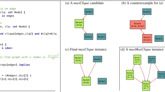
(a) A maxClique candidate (b) A counterexample for (a)
(c) Final maxClique instance (d) A maxMaxClique instance
Figure 2. Automatically generated sample instances satisfying
the maxClique and maxMaxClique predicates. At this pointclq2could have been anything that is either
not a clique or not larger thanclq.
2. Next, Alloy* attempts to falsify the previous candidate
by finding, again, only one set of nodes clq2, but this
time such thatclq2is a clique in larger thanclq, for the
exact (concrete) graph found in the previous step. In this case, it finds one such counterexample clique (red nodes in Figure 2(b)) refuting the proposition thatclqfrom the
first step is a maximum clique.
3. Alloy* continues by trying to find another candidate clique, encoding the knowledge gained from the previous counterexample (explained in more detail in Section 3 and 4) to prune the remainder of the search space. After a couple of iterations, it finds the candidate in Figure 2(c) which cannot be refuted, so it returns that candidate as a satisfying solution.
Alloy* handles higher-order quantifiers in a generic and model-agnostic way, meaning that it allows higher-order quantifiers to appear anywhere where allowed by the Al-loy syntax, and does not require any special idiom to be
fol-lowed. Once written, themaxCliquepredicate (despite
con-taining a higher-order quantification) can be used in other parts of the model, like any other predicate, just as we used it to formulate and check Turán’s theorem.
Using a order predicate inside another higher-order predicate is also possible. It might not be obvious that theTurancheck contains nested higher-order quantifiers, so
a simpler example would be finding a max clique with a maximum sum of node values:
sigNode { val:one Int}
// Auxiliary function: returns the sum of all node values
funvalsum[nodes:setNode]: Int{sumn: nodes | n.val } // ’clq’ is a max clique with maximum sum of node values
predmaxMaxClique[edges: Node -> Node, clq:setNode] {
maxClique[edges, clq]
no clq2:setNode |
clq2!=clqandmaxClique[edges,clq] andvalsum[clq2]>valsum[clq] }
runmaxMaxCliquefor5
Running themaxMaxCliquecommand spawns 2 nested CEGIS
loops; every candidate instance and counterexample gener-ated in the process can be opened and inspected in the stan-dard Alloy visualizer. A sample generated instance is shown in Figure 2(d).
2.2 Policy Synthesis
Policy design and analysis is an active area of research. A number of existing tools [11, 14, 27, 33] use a declarative language to specify policies, and a constraint-based analysis to verify them against a high-level property. In this section, we demonstrate how Alloy* can be used to automatically synthesize a policy that satisfies given properties.
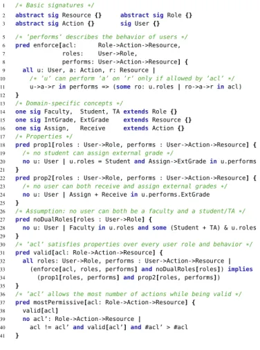
Figure 3 shows an Alloy model that describes the problem of grade assignment at a university, based on the running ex-ample from [11]. A policy specification contains three basic concepts: roles, actions, and resources. A system consists of a set of users, each having one or more roles and performing some actions on a set of resources. A policy (acl) is a set of
tuples fromRoletoActiontoResource, describing a set of
allowed actions. For example, a policy containing only a sin-gle tupleFaculty->Assign->ExtGrademeans that a user may
assign an external grade only if it has theFacultyrole.
There are two desirable properties over this system: (1) students should not be able to assign external grades, and (2) no user should be able to both assign and receive external grades. A policy is considered valid if and only if, when quantified over every possible combination of user roles and behaviors, it ensures that the properties hold. This higher-order property is encoded in thevalidpredicate.
Running Alloy* to search for an instance satisfying the
validpredicate completes in about 0.5 seconds, and retuns
an empty policy, which is technically valid but not very use-ful (since it allows no actions to be performed by anyone!). Fortunately, we can leverage the higher-order featur of Al-loy* to synthesize more interesting policies. For example, 3 additional lines of Alloy are enough to describe the most permissive policy as a policy that is valid such that no other valid policy has more tuples in it (lines 39–41). It takes about 3.5 seconds to generate one such policy:
{Faculty,Receive,ExtGrade}, {Faculty,Assign,Resource}, {Student,Receive,Resource}, {Student,Assign,IntGrade},
{TA,Receive,Resource}, {TA,Assign,IntGrade}
This policy provides a starting point for further exploration of the policy space. The designer may decide, for example,
that students should not be able to assign IntGrade, add
another property, and then repeat the synthesis process.
1 /* Basic signatures */ 2 abstract sigResource {}
3 abstract sigAction {}
abstract sigRole {}
sigUser {}
5 /* ’performs’ describes the behavior of users */ 6 predenforce[acl: Role->Action->Resource,
7 roles: User->Role,
8 performs: User->Action->Resource] {
9 allu: User, a: Action, r: Resource |
10 /* ’u’ can perform ’a’ on ’r’ only if allowed by ’acl’ */ 11 u->a->rin performs => (somero: u.roles | ro->a->rinacl)
12 }
13 /* Domain-specific concepts */
14 one sigFaculty, Student, TA extendsRole {}
15 one sigIntGrade, ExtGrade extendsResource {}
16 one sigAssign, Receive extendsAction {}
17 /* Properties */
18 predprop1[roles : User->Role, performs : User->Action->Resource] {
19 /* no student can assign external grade */
20 no u: User | u.roles = StudentandAssign->ExtGradein u.performs
21 }
22 predprop2[roles : User->Role, performs : User->Action->Resource] {
23 /* no user can both receive and assign external grades */ 24 no u: User | Assign + Receiveinu.performs.ExtGrade
25 }
26 /* Assumption: no user can both be a faculty and a student/TA */ 27 prednoDualRoles[roles : User->Role] {
28 no u: User | Facultyinu.rolesand some(Student + TA) & u.roles
29 }
30 /* ’acl’ satisfies properties over every user role and behavior */ 31 predvalid[acl: Role->Action->Resource] {
32 allroles: User->Role, performs : User->Action->Resource |
33 (enforce[acl, roles, performs]andnoDualRoles[roles])implies
34 (prop1[roles, performs]andprop2[roles, performs])
35 }
36 /* ’acl’ allows the most number of actions while being valid */ 37 predmostPermissive[acl: Role->Action->Resource] {
38 valid[acl]
39 no acl’: Role->Action->Resource |
40 acl != acl’andvalid[acl’] and#acl’ > #acl
41 }
Figure 3. Grade Assignment Policy in Alloy*
3. Background and Key Ideas
Skolemization Many first-order constraint solvers allow some form of higher-order quantifiers to appear at the lan-guage level. Part of the reason for this is that, in certain cases, quantifiers can be eliminated in a preprocessing step
called skolemization. In a model finding setting, every top-level existential quantifier is eliminated by (1) introducing a skolem constant for the quantification variable, and (2) replacing every occurrence of that variable with the newly created skolem constant. For example, solving the following higher-order formula
some s: set univ | #s > 2
means finding one setswith more than 2 elements, i.e., $s in univ && #$s > 2,
which is first-order and thus solvable by general purpose constraint solvers. (Throughout, following the convention of the Alloy Analyzer, skolem constants will be identified with a dollar sign as a prefix.)
CEGIS CounterExample-Guided Inductive Synthesis [36] is an approach for solving higher-order synthesis problems, which is extended in Alloy* to the general problem of solv-ing higher-order formulas. The goal of CEGIS is to find one instance (e.g., a program) that satisfies some property for all possible environments (e.g., input values):
some p: Program | all env: Var->Int | spec[p, env].
Step 1: Search. Since this formula is not immediately solvable by today’s state-of-the-art solvers, the CEGIS strat-egy is to first find a candidate program and one environment for which the property holds:
some p: Program | some env: Var->Int | spec[p, env].
This formula is amenable to automated first-order constraint solving, as both quantifiers can now be skolemized.
Step 2: Verification. If a candidate is found, the next step is to check whether that candidate might actually satisfy the specification for all possible environments. The verification condition, thus, becomes
all env: Var->Int | spec[$p, env].
The outer quantifier from the previous step (some p: Program)
is not present in this formulation, because the verification condition is to be checked for exactly the candidate program
generated in Step 1 (the concrete program$p). This check
is typically done by refutation, that is, by trying to find a counterexample for which the verification condition does not hold. Negating the verification condition and pushing the negation through to the leaf nodes changes the quantifier
fromalltosome, which becomes skolemizable, resulting in
a first order formula that is now easily solved:
some env: Var->Int | not spec[$p, env]
Step 3: Induction. The previous step either verifies the candidate or returns a counterexample—a concrete environ-ment for which the program does not satisfy the spec. In-stead of simply continuing the search for some other can-didate program and repeating the whole procedure, a key idea behind the CEGIS method is adding an encoding of the counterexample to the original candidate condition:
some p: Program | some env: Var->Int |
spec[p, env] && spec[p, $env_cex]
Consequently, all subsequent candidate programs will have
to satisfy the spec for the concrete environment$env_cex.
This strategy in particular tends to be very effective at reduc-ing the search space and improvreduc-ing the overall scalability. CEGIS for a general purpose solver. Existing CEGIS-based synthesis tools implement this strategy internally, op-timizing for the target domain of synthesis problems. A key insight of this paper is that the CEGIS strategy can be implemented, generically and efficiently, inside a general purpose constraint solver. For an efficient implementation, however, it is important that such a solver be optimized with the following features:
•Partial Instances. The verification step requires that the verification condition be solved against the previously discovered candidate; being able to explicitly set that can-didate as a part of the solution to the verification problem known upfront (i.e., as a “partial instance”) tends to be significantly more efficient than encoding the candidate with constraints [40].
•Incremental solving. Except for one additional constraint, the induction step solves exactly the same formula as the search step. Many modern SAT solvers already allow new constraints to be added to already solved propositional formulas, making subsequent runs more efficient (be-cause all previously learned clauses are readily reusable).
•Atoms as expressions. The induction step needs to be
able to convert a concrete counterexample (given in terms of concrete atoms, i.e., values for each variable) to a formula to be added to the candidate search condition. All atoms, therefore, must be convertible to expressions. This is trivial for SAT solvers, but requires extra functionality for solvers offering a richer input language.
•Skolemization. Skolemizing higher-order existential
quan-tifiers is necessary for all three CEGIS steps.
We formalize our approach in Section 4, assuming availabil-ity of a first-order constraint solver offering all the features above. In Section 5 we present our implementation as an extension to Kodkod [38] (a first-order relational constraint solver already equipped with most of the required features).
4. Semantics
We give the semantics of our decision procedure for bounded higher-order logic (as implemented in Alloy*) in two steps. First, we formalize the translation of a boolean (possibly
higher-order) formula into aProcdatatype instance
(corre-sponding to an appropriate solving strategy); next we for-malize the semantics ofProcsatisfiability solving.
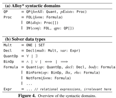
Figure 4 gives an overview of all syntactic domains used throughout this section. We assume the datatypes in
Fig-(a) Alloy* syntactic domains
QP = QP(forAll: Quant, pExists: Proc)
Proc = FOL(form: Formula)
| OR(disjs: Proc[])
| E A(conj: FOL, qps: QP[])
(b) Solver data types
Mult = ONE | SET
Decl = Decl(mult: Mult, var: Expr) QuantOp = ∀ | ∃
BinOp = ∧ | ∨ | ⇐⇒ | Ô⇒
Formula = Quant(op: QuantOp, decl: Decl, body: Formula)
| BinForm(op: BinOp, lhs, rhs: Formula)
| NotForm(form: Formula)
| ...
Expr = ... // relational expressions, irrelevant here
Figure 4. Overview of the syntactic domains. (a) Semantic functions
T : Formula→Proc top-level formula translation
S : Proc→Instance Procevaluation (solving)
τ : Formula→Proc intermediate formula translation
⋏ : Proc→Proc→Proc Proccomposition: conjunction
⋎ : Proc→Proc→Proc Proccomposition: disjunction
(b) Functions exported by first-order solver
solve : Formula→Instance option first-order solver
eval : Instance→Expr→Value evaluator
replace : Formula→Expr→Value→Formula
nnf : Formula→Formula NNF conversion
skolemize : Formula→Formula skolemization
∧ : Formula→Formula→Formula conjunction
∨ : Formula→Formula→Formula disjunction
TRUE : Formula true formula
FALSE : Formula false formula
(c) Built-in functions
fold : (A → E → A)→A→E[]→A functional fold
reduce : (A → E → A)→E[]→A fold w/o init value
map : (E → T)→E[]→T[] functional map
length : E[]→int list length
hd : E[]→E list head
tl : E[]→E[] list tail
+ : E[]→E[]→E[] list concatenation
× : E[]→E[]→E[] list cross product
fail : String→void runtime error
Figure 5. Overview of used functions: (a) semantic functions, (b) functions provided by the first-order solver, (c) built-in functions. ure 4(b) are provided by the solver; on top of these basic datatypes, Alloy* defines the following additional datatypes:
•FOL—a wrapper for a first-order formula that can be
solved in one step by the solver;
• E A—a composite type representing a conjunction of a first-order formula and a number of higher-order
univer-sal quantifiers (each enclosed in aQPdatatype). The
in-tention of theQPdatatype is to hold the original univer-sally quantified formula (the forAll field), and a transla-tion of the same formula but quantified existentially (the pExists field); the latter is later used to find candidate so-lutions (formalized in Section 4.2).
Figure 5(a) lists all the semantic functions defined in this paper. The main two are translation of formulas into Procs (T , defined in Figure 6) and satisfiability solving (S, defined in Figure 7). Relevant functions exported by the solver are given in Figure 5(b), while other functions, assumed to be provided by the host programming language, are summarized in Figures 5(c).
For simplicity of exposition, we decided to exclude the treatment of bounds from our formalization, as it tends to be mostly straightforward; we will, however, come back to this point and accurately describe how the bounds are constructed before a solver invocation.
Syntax note. Our notation is reminiscent of ML. We use the “.” syntax to refer to field values of datatype instances. If the left-hand side in such constructs resolves to a list, we assume the operation is mapped over the entire list (e.g., ea.qps.forAll, is equivalent to map λq⋅ q.forAll, ea.qps). 4.1 Translation of Formulas into Proc Objects
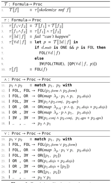
The top-level translation function (T , Figure 6, line 1) en-sures that the formula is converted to Negation Normal Form (NNF), and that all top-level existential quantifiers are sub-sequently skolemized away, before the formula is passed to the τ function. Conversion to NNF pushes the quantifiers towards the roots of the formula, while skolemization elim-inates top-level existential quantifiers (including the higher-order ones). Alloy* aggressively uses these techniques to achieve completeness in handling arbitrary formulas.
Translating a binary formula (which must be either a con-junction or discon-junction, since it is in NNF) involves translat-ing both left-hand and right-hand sides and compostranslat-ing the
resultingProcs using the corresponding composition
opera-tor (⋏ for conjunction, and ⋎ for disjunction, lines 2–3). An important difference between the two cases, however, is that a disjunction demands that both sides be skolemized again (thus the use of T instead of τ), since they were surely un-reachable by any previous skolemization attempts. This en-sures that any higher-order quantifiers found in a clause of a disjunction will eventually either be skolemized or converted to an E AProc.
A first-order universal quantifier (determined by d.mult
being equal toONE) whose body is also first-order (line 6)
is simply enclosed in a FOL Proc (line 7). Otherwise, an
E A
Proc is returned, wrapping both the original formula
(∀d ∣ f) and the translation of its existential counterpart (p = T J∃d ∣ fK). The existential version is later used to find
T : Formula→Proc
1. T JfK ≡ τJskolemize nnf fK
τ : Formula→Proc
2. τJf1∨f2K ≡ T Jf1K ⋎ T Jf2K 3. τJf1∧f2K ≡ τJf1K ⋏ τJf2K
4. τJ∃d ∣ fK ≡ fail “can’t happen”
5. τJ∀d ∣ fK ≡ let p = T J∃d ∣ fK in
6. if d.mult is ONE && p is FOL then
7. FOL(∀d ∣ f)
8. else
9. E A(FOL(TRUE), [QP(∀d ∣ f, p)])
10. τJfK ≡ FOL(f)
⋏ : Proc→Proc→Proc
11. p1⋏ p2 ≡ match p1, p2 with
12. | FOL, FOL→ FOL(p1.form∧ p2.form)
13. | FOL, OR → OR(map λp⋅ p1⋏ p, p2.disjs)
14. | FOL, E A → E A(p1⋏p2.conj, p2.qps)
15. | OR , OR → OR(map λp,q⋅ p ⋏ q, p1.disjs× p2.disjs)
16. | OR , E A → OR(map λp⋅ p ⋏ p1, p1.disjs)
17. | E A , E A → E A(p1.conj⋏ p2.conj, p1.qps+ p2.qps)
18. | _ , _ → p2⋏ p1
⋎ : Proc→Proc→Proc
19. p1⋎ p2 ≡ match p1, p2 with
20. | FOL, FOL→ FOL(p1.form∨ p2.form)
21. | FOL, OR → OR(map λp⋅ p1⋎ p, p2.disjs)
22. | FOL, E A → OR([p1, p2])
23. | OR , OR → OR(p1.disjs+ p2.disjs)
24. | OR , E A → OR(p1.disjs+ [p2])
25. | E A , E A → OR([p1, p2])
26. | _ , _ → p2⋎ p1
Figure 6. Translation of booleanFormulas toProcs. candidate solutions (which satisfy the body for some binding for d), whereas the original formula is needed when check-ing whether generated candidates also satisfy the property for all possible bindings (i.e., the verification condition).
In all other cases, the formula is wrapped inFOL(line 10).
4.1.1 Composition ofProcs
Composition ofProcs is straightforward for the most part,
directly following the distributivity laws of conjunction over disjunction and vice versa. The common goal in all the cases
in lines 11–26 is to reduce the number ofProcnodes. For
example, instead of creating anOR node for a disjunction
of two first-order formulas (line 20), aFOLnode is created
containing a disjunction of the two. Other interesting cases
involve the E AProc. A conjunction of two E Anodes can be
merged into a single E Anode (line 17), as can a conjunction
of aFOLand an E A node (line 14). A disjunction involving
S : Proc→Instance option
27. SJpK ≡ match p with
28. | FOL→ solve p.form
29. | OR → if length p.disjs = 0 then None else match SJhd p.disjsK with
30. | None → SJOR(tl p.disjs)K
31. | Some(inst) →Some(inst)
32. | E A → let pcand = fold ⋏, p.conj, p.qps.pExists in
33. match SJpcandK with
34. | None → None
35. | Some(cand)→ let fcheck = fold ∧, TRUE, p.qps.forAll in
36. match SJT J¬fcheckKK with
37. | None → Some(cand)
38. | Some(cex)→ fun repl(q) = replace(q.body, q.decl.var, eval(cex, q.decl.var))
39. let f∗
cex = map repl, p.qps.forAll in
40. let fcex = fold ∧, TRUE, fcex∗ in
41. SJpcand⋏ T JfcexKK
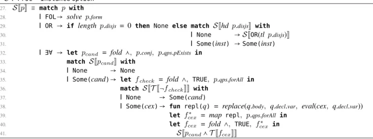
Figure 7. Satisfiability solving for differentProcs. The resultingInstanceobject encodes the solution, if one is found. 4.2 Satisfiability Solving
The procedure for satisfiability solving is given in Figure 7.
A first-order formula (enclosed in FOL) is given to the
solver to be solved directly, in one step (line 28).
AnOR Procis solved by iteratively solving its disjuncts
(lines 29–31). An instance is returned as soon as one is
found; otherwise,Noneis returned.
The procedure for the E A Procs implements the CEGIS
loop (lines 32–41). The candidate search condition is a con-junction of the first-order p.conjProcand all the existential
Procs from p.qps.pExists(line 32). If solving the candidate
condition returns no instance, the formula as a whole is un-satisfiable (line 34). If a candidate is found, the procedure checks whether that candidate actually satisfies all possible bindings for the involved quantifiers. The verification condi-tion (fcheck) becomes a conjunction of all original universal quantifiers within this E A(line 35). The procedure proceeds by trying to refute this proposition, that is, by attempting to satisfy the negation of the verification condition (line 36). If the refutation step is unsuccessful (line 37), the previously discovered candidate is returned as a satisfying instance for the formula as a whole; otherwise, the search continues by asking for another candidate which additionally satisfies the returned counterexample (line 41). Encoding the counterex-ample into a formula boils down to obtaining a concrete value that each quantification variable has in that counterex-ample (by means of calling the eval function exported by the solver) and embedding that value directly in the body of the corresponding quantifier (lines 38-40).
4.3 Treatment of Bounds
Bounds are a required input of any bounded analysis; for an analysis involving structures, the bounds may include not only the cardinality of the structures, but may also indicate that a structure includes or excludes particular tuples. Such
bounds serve not only to finitize the universe of discourse and the domain of each variable, but may also specify a partial instance that embodies information known upfront about the solution to the constraint. If supported by the solver, specifying the partial instance through bounds (as opposed to enforcing it with constraints) is an important mechanism that generally improves scalability significantly. Although essential, the treatment of bounds in Alloy* is mostly straightforward—including it in the above formaliza-tion (Figures 6 and 7) would only clutter the presentaformaliza-tion and obscure the semantics of our approach. Instead, we in-formally (but precisely) provide the relevant details in the rest of this section.
Bounds may change during the translation phase by means of skolemization: every time an existential quantifier is skolemized, a fresh variable is introduced for the quantifi-cation variable and a bound for it is added. Therefore, we
associate bounds withProcs, as differentProcs may have
different bounds. Whenever a composition of twoProcs is
performed, the resultingProcgets the union of the two
cor-responding bounds.
During the solving phase, whenever the solve function is applied (line 28), bounds must be provided as an argument—
we simply use the bounds associated with the inputProc
in-stance (p). When supplying bounds for the translation of the verification condition (T J¬fcheckK, line 36), it is essential to encode the candidate solution (cand) as a partial instance, to ensure that the check is performed against that particular candidate, and not some other arbitrary one. That is done by
bounding every variable from p.boundsto the exact value it
was given in cand:
fun add_bound(b, var) = b + r ↦ eval(cand, var)
bcheck= foldadd_bound, p.bounds, p.bounds.variables Finally, when translating the formula obtained from the
candidate (line 41), the same bounds are used as for the current candidate (pcand.bounds).
5. Implementation
We implemented our decision procedure for higher-order constraint solving as an extension to Kodkod [38]. Kodkod, the backend engine used by the Alloy Analyzer, is a bounded constraint solver for relational first-order logic (thus, ‘vari-able’, as used previously, translates to ‘relation’ in Kodkod, and ‘value’ translates to ‘tuple set’). It works by translating a given relational formula (together with bounds finitizing relation domains) into an equisatisfiable propositional for-mula and using an of-the-shelf SAT solver to check its satis-fiability. The Alloy Analyzer delegates all its model finding (constraint solving) tasks to Kodkod. No change was needed to the Alloy Analyzer’s existing translation from the Al-loy modeling language to the intermediate logic of Kodkod; loosening Kodkod’s restrictions on higher-order quantifica-tion exposes the new funcquantifica-tionality immediately at the level of Alloy models.
The official Kodkod distribution already offers most of the required features identified in Section 3. While effi-cient support for partial instances has always been an in-tegral part of Kodkod, only the latest version (2.0) comes with incremental SAT solvers and allows new relational con-straints, as well as new relations, to be added incrementally to previously solved problems. By default, Kodkod performs skolemization of top-level existential quantifiers (including higher-order ones); the semantics of our translation from
boolean formulas to Procs ensures that all quantifiers,
re-gardless of their position in the formula, eventually get pro-moted to the top level, where they will be subject to skolem-ization.
Conversion from atoms to expressions, however, was not available in Kodkod prior to this work. Kodkod imposes a strict separation between the two abstractions; doing so allows it to treat all atoms from a single relation domain as indistinguishable from each other, which helps generate a stronger symmetry-breaking predicate. Since encoding each counterexample back to the candidate condition is absolutely crucial for CEGIS to scale, we extended Kodkod with the ability to create a singleton relation for each declared atom, after which converting atoms back to expressions (relations) becomes trivial. We also updated the symmetry-breaking predicate generator to ignore all such singleton relations that are not used in the formula being solved. As a result, this modification does not seem to incur any performance overhead; we ran the existing Kodkod test suite with and without the modification and observed no time difference (in both cases the total time it took to run 249 tests was around 230s).
Aside from the fact that it is written in Java, our imple-mentation directly follows the semantics defined in Figures 6 and 7. Additionally, it performs the following important
op-timizations: (1) the constructor forORdata type finds allFOL Procs in the list of received disjuncts and merges them into one, and (2) it uses incremental solving to implement line 41 from Figure 7 whenever possible.
6. Case Study: Program Synthesis
Program synthesis is one of the most popular applications of higher-order constraint solving. The goal of program synthe-sis is to produce a program that satisfies a given (high-level) specification. Synthesizers typically also require a loose def-inition of the target program’s structure, and most use an ad hoc CEGIS loop relying on an off-the-shelf first-order con-straint solver to generate and verify candidate programs.
The SyGuS [3] (syntax-guided synthesis) project has pro-posed an extension to SMTLIB for encoding program syn-thesis problems. The project has also organized a competi-tion between solvers for the format, and provides three ref-erence solvers for testing purposes.
We encoded a subset of the SyGuS benchmarks in Al-loy* to test its scalability. These benchmarks have a standard format, are well tested, and allow comparison to the perfor-mance of the reference solvers, making them a good target for evaluating Alloy*. We found that Alloy* scales better than all three of the reference solvers.
6.1 Example Encoding
To demonstrate our strategy for encoding program synthesis problems in Alloy*, we present the Alloy* specification for the problem of finding a program to compute the maximum
of two numbers (themax-2benchmark). The original SyGuS
encoding of the benchmark is reproduced in Figure 8. (synth-fun max2 ((x Int) (y Int)) Int
((Start Int (x y 0 1 (+ Start Start) (- Start Start) (ite StartBool Start Start)))
(StartBool Bool ((and StartBool StartBool)(or StartBool StartBool) (not StartBool)
(<= Start Start)(= Start Start)(>= Start Start))))) (declare-var x Int)
(declare-var y Int)
(constraint (>= (max2 x y) x)) (constraint (>= (max2 x y) y))
(constraint (or (= x (max2 x y)) (= y (max2 x y))))
Figure 8. max-2benchmark from the SyGuS project.
We encode themax-2benchmark in Alloy* using
signa-tures to represent the production rules of the program gram-mar, and predicates to represent both the semantics of pro-grams and the constraints restricting the target program’s se-mantics. Programs are composed of abstract syntax nodes, which can be integer- or boolean-typed.
abstract sigNode {}
abstract sigIntNode, BoolNodeextendsNode {}
abstract sigVar extendsIntNode {}
one sigX, YextendsVar {}
sigITEextendsIntNode { condition: BoolNode, then, elsen: IntNode, }
sigGTEextendsBoolNode { left, right: IntNode }
Integer-typed nodes include variables and if-then-else ex-pressions, while boolean-typed nodes include greater-than-or-equal expressions. Programs in this space evaluate to in-tegers or booleans; inin-tegers are built into Alloy, but we must model boolean values ourselves.
abstract sigBool {}
one sigBoolTrue, BoolFalse extendsBool {}
The standard evaluation semantics of these programs can be encoded in a predicate that constrains the evaluation re-lation. It works by constraining all compound syntax tree nodes based on the results of evaluating their children, but does not constrain the values of variables, allowing them to range over all values.
predsemantics[eval: Node -> (Int+ Bool)] {
alln: ITE | eval[n]in Int and
eval[n.condition] = BoolTrueimplies
eval[n.then] = eval[n]elseeval[n.elsen] = eval[n]
alln: GTE | eval[n]in Booland
eval[n.left] >= eval[n.right]implies
eval[n] = BoolTrueelseeval[n] = BoolFalse
allv: Var |oneeval[v]andeval[v]in Int
}
The program specification says that the maximum of two numbers is greater than or equal to both numbers, and that the result is one of the two.
predspec[root: Node, eval: Node -> (Int+ Bool)] { (eval[root] >= eval[X]andeval[root] >= eval[Y])and
(eval[root] = eval[X] oreval[root] = eval[Y]) }
Finally, the problem itself requires solving for some ab-stract syntax tree such that for all valid evaluation relations (i.e. all possible valuations for the variables), the specifica-tion holds.
predsynth[root: IntNode] {
alleval: Node -> (Int+ Bool) |
semantics[eval]impliesspec[root, eval] }
(A.1) runsynthfor4but2Int
We present the results of our evaluation, including a per-formance comparison between Alloy* and existing program synthesizers, in Section 8.2.
7. Optimizations
Originally motivated by the formalization of the synthesis problem (as presented in Section 6), we designed and imple-mented two general purpose optimization for Alloy*. 7.1 Quantifier Domain Constraints
As defined in Listing A.1, thesynthpredicate, although
log-ically sound, suffers from serious performance issues. The most obvious reason is how the implication inside the univer-sal higher-order quantifier (“the semantics implies the spec”) affects the CEGIS loop. To trivially satisfy the implication, the candidate search step can simply return and instance for which the semantics does not hold. Furthermore, adding the
encoding of the counterexample refuting the previous in-stance is not going to constrain the next search step to find a program and a valuation for which the spec holds. This cycle can go on for unacceptably many iterations.
This reflects an old philosophical problem in first-order logic: “all men are mortal" is only equivalent to “for all x, if x is a man, then x is mortal” in a rather narrow, model-theoretic sense. The case of a non-man being non-mortal is a witness to the second but not to the first.
To overcome this problem, we can add syntax to identify the constraints that should be treated as part of the bounds of
a quantification. Thesynthpredicate now becomes
pred synth[root: IntNode] {
alleval: Node -> (Int+ Bool)whensemantics[eval] | spec[root, eval]
}
The existing first-order semantics of Alloy is unaffected, i.e., all xwhenD[x] | P[x] ⇐⇒ all x | D[x]impliesP[x]
some xwhenD[x] | P[x] ⇐⇒ somex | D[x]andP[x] (A.2) The rule for pushing negation through quantifiers (used by the converter to NNF) becomes:
not(all xwhenD[x] | P[x]) ⇐⇒ somex whenD[x] |notP[x]
not(somexwhenD[x] | P[x]) ⇐⇒ all x whenD[x] |notP[x] (which is consistent with classical logic).
The formalization of the Alloy* semantics needs only a minimal change. The change in semantics is caused by es-sentially not changing how the existential counterpart of a universal quantifier is obtained— only by flipping the quan-tifier, and keeping the domain and the body the same (line 5, Figure 6). Consequently, the candidate condition always searches for an instance satisfying both the domain and the body constraint (or in terms of the synthesis example, both the semantics and the spec). The same is automatically true for counterexamples obtained in the verification step. The only actual change to be made to the formalization is
ex-panding q.body in line 38 according to the rules in
List-ing A.2.
Going back to the synthesis example, even after rewriting thesynthpredicate, unnecessary overhead is still incurred
by quantifying over valuations for all the nodes, instead of valuations for just the input variables. Another consequence is that the counterexamples produced in the CEGIS loop do not guide the search as effectively. This observation leads
us to our final formulation of thesynthpredicate, which we
used in all benchmarks presented in Section 8.2: pred synth[root: IntNode] {
allenv: Var ->Int|
someeval: Node -> (Int+ Bool)when
envineval && semantics[eval] | spec[root, eval]
}
(A.3) Even though it uses nested higher-order quantifiers, it turns out to be the most efficient. The reason is that the in-nermost quantifier (overeval) always takes exactly one
iter-ation (to either prove or disprove the currentenv), because
7.2 Strictly First-Order Increments
We already pointed out the importance of implementing the induction step (line 41, Figure 7) using incremental SAT solving. A problem, however, arises when the encoding of the counterexample (as defined in lines 38-40) is not a first-order formula—since not directly translatable to SAT, it can-not be incrementally added to the existing SAT translation of the candidate search condition (pcand). In such cases, the
se-mantics in Figure 7 demands that the conjunction of pcand
and T JfcexK be solved from scratch, loosing any benefits
from previously learned SAT clauses.
This problem occurs in our final formulation of thesynth
predicate (Listing A.3), due to the nested higher-order quan-tifiers. To address this issue, we relax the semantics of the in-duction step by replacing SJpcand⋏T JfcexKK (line 41) with
fun Tfo(f) = match p = T JfK with
| FOL → p
| OR → reduce ⋎, map(Tfo, p.disjs)
| EA → fold ⋏, p.conj, map(Tfo, p.qps.pExists)
SJpcand⋏ Tfo(fcex)K
The Tfofunction ensures that fcexis translated to a
first-orderProc, which can always be added as an increment to
the current SAT translation of the candidate condition. The trade-off involved here is that this new encoding of the coun-terexample is potentially not as strong, and therefore may lead to more CEGIS iterations before a resolution is reached. For that reason, Alloy* accepts a configuration parameter (accessible via the “Options” menu), offering both seman-tics. In Section 8 we provide experimental data showing that for all of our synthesis examples, the strictly first-order in-crements yielded better performance.
8. Evaluation
8.1 Micro Benchmarks
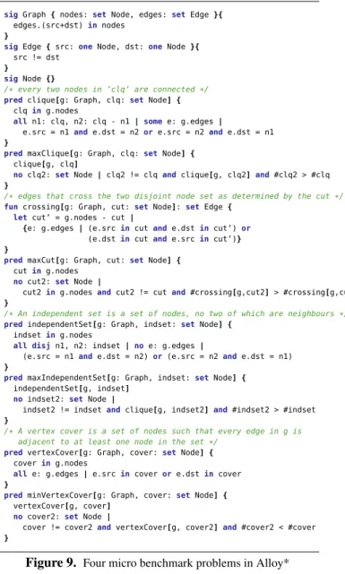
To assess how well Alloy* scales on higher-order graph problems, we selected the following 4 classical problems:
max clique, max cut, max independent set, and min vertex cover. We specified each of the four problems in Alloy*
(see Figure 9 for the full Alloy specification), and executed them on a set of pre-generated graphs, measuring the perfor-mance of the tool in successfully producing a correct output. It can be expected that verification problems requiring the discovery of a graph with such properties would require comparable computational resources.
Experiment Setup We used the Erd˝os-Rényi model [9] to randomly generate graphs to serve as inputs to the bench-mark problems. To cover graphs with a wide range of den-sities, we used 5 probabilities (0.1, 0.3, 0.5, 0.7, 0.9) for in-serting an edge between a pair of nodes in a graph. In total, we generated 210 different graphs, with sizes ranging from 2 to 50 nodes.
To additionally test the correctness of our implementa-tion, we compared the results return by Alloy* to those of
sigGraph { nodes: setNode, edges:setEdge }{ edges.(src+dst)in nodes
}
sigEdge { src: oneNode, dst:oneNode }{ src != dst
}
sigNode {}
/* every two nodes in ’clq’ are connected */
pred clique[g: Graph, clq:setNode] { clqing.nodes
alln1: clq, n2: clq - n1 |somee: g.edges |
e.src = n1 ande.dst = n2ore.src = n2 ande.dst = n1 }
pred maxClique[g: Graph, clq:setNode] { clique[g, clq]
no clq2:setNode | clq2 != clqandclique[g, clq2]and#clq2 > #clq }
/* edges that cross the two disjoint node set as determined by the cut */
funcrossing[g: Graph, cut:setNode]: setEdge {
letcut’ = g.nodes - cut |
{e: g.edges | (e.src incutande.dstin cut’)or
(e.dst incutande.srcin cut’)} }
pred maxCut[g: Graph, cut:setNode] { cuting.nodes
no cut2:setNode |
cut2in g.nodesandcut2 != cutand#crossing[g,cut2] > #crossing[g,cut] }
/* An independent set is a set of nodes, no two of which are neighbours */
pred independentSet[g: Graph, indset:setNode] { indsetin g.nodes
all disjn1, n2: indset |no e: g.edges |
(e.src = n1 ande.dst = n2)or (e.src = n2ande.dst = n1) }
pred maxIndependentSet[g: Graph, indset:setNode] { independentSet[g, indset]
no indset2:setNode |
indset2 != indsetandclique[g, indset2]and#indset2 > #indset }
/* A vertex cover is a set of nodes such that every edge in g is adjacent to at least one node in the set */
pred vertexCover[g: Graph, cover:setNode] { coverin g.nodes
alle: g.edges | e.srcincover ore.dst incover }
pred minVertexCover[g: Graph, cover:setNode] { vertexCover[g, cover]
no cover2:setNode |
cover != cover2 andvertexCover[g, cover2]and#cover2 < #cover }
Figure 9. Four micro benchmark problems in Alloy*
known imperative algorithms for the above problems1 and
made sure they matched. The timeout for each run (solving a single problem for a given graph) was set to 100 seconds. Results Figure 10 plots the average solving time across graphs size. The results show that for all problems but
max cut, Alloy* was able to handle graphs of sizes up to
50 nodes in less than a minute (max cutstarted to time out at
around 25 nodes). Our original goal for this benchmarks was to be able to solve graphs with 10-15 nodes, and claim that Alloy* can be effectively used for teaching, specification animation, and small scope checking, all within the Alloy Analyzer GUI (which is one of the most common uses of the Alloy technology). These results, however, indicate that executing higher-order specifications can be feasible even
1Formax cliqueandmax independent set, we used the Bron-Kerbosch
heuristic algorithm; for the other two, no good heuristic algorithm is known, and so we implemented enumerative search. In both cases, we used Java.
0 10 20 30 40 50 60 70 80 2 3 5 7 9 13 15 20 25 30 35 40 45 50 So lv in g T im e (s ) # Nodes max clique max cut max indep. set min vertex cover
Figure 10. Average solving times for benchmark algorithms
0 2 4 6 8 10 12 14 2 3 5 7 9 13 15 20 25 30 35 40 45 50 # C an d id ate s # Nodes max clique max cut max indep. set min vertex cover
Figure 11. Average number of candidates considered for bench-mark algorithms
for declarative programming (where a constraint solver is integrated with a programming language, e.g., [25, 26]), which is very encouraging.
Figure 11 shows the average number of candidate solu-tions Alloy* explored before producing a final output. As the graph size became larger, the number of candidates also increased, but in most cases, Alloy* was able to find a cor-rect solution under 6 candidates. One exception was the max cut problem: For graphs of size 25, Alloy* considered up to 13 candidates, after which the resulting constraints became too hard for the SAT solver, leading to a timeout.
Figure 12 show average solving times for individual prob-ability thresholds used to generate graphs for the micro benchmark experiments. Lower the threshold (T), denser the graph is (similarly, higher T values lead to sparser graphs). In general, the solving time tends to be greater for denser graphs, as the search space is bigger. This trend is espe-cially evident in the max cut problem (Figure 12(b)), where the solving time increases drastically for T=0.1 until Alloy* times out at graphs of size 20.
On the other hand, sparsity does not necessarily lead to faster performance. For example, in the max clique and max independent set, note how Alloy* takes longer on graphs with T=0.9 (Figures 12(a) and (c)) than on those with lower threshold as the graph size increases. We believe that this
0 10 20 30 40 50 60 70 80 2 3 5 7 9 13 15 20 25 30 35 40 45 50 So lv in g T im e (s ) # Nodes T=0.1 T=0.3 T=0.5 T=0.7 T=0.9
(a)max clique
0 20 40 60 80 100 120 140 2 3 5 7 9 13 15 20 25 So lv in g Ti me ( s) # Nodes T=0.1 T=0.3 T=0.5 T=0.7 T=0.9 (b)max cut 0 10 20 30 40 50 60 2 3 5 7 9 13 15 20 25 30 35 40 45 50 So lv in g T im e (s ) # Nodes T=0.1 T=0.3 T=0.5 T=0.7 T=0.9
(c)max independent set
0 0.2 0.4 0.6 0.8 1 1.2 1.4 1.6 1.8 2 3 5 7 9 13 15 20 25 30 35 40 45 50 So lv in g T im e (s ) # Nodes T=0.1 T=0.3 T=0.5 T=0.7 T=0.9
(d)min vertex cover
Figure 12. Avg. times per each threshold for graph benchmarks is because sparser graphs tend to permit fewer cliques (and independent sets) than more densely connected graphs. 8.2 Program Synthesis
Out of 124 total benchmarks in the SyGuS project, we en-coded the 10 that do not involve bit vectors and compared the performance of Alloy* in finding correct programs to that
of the provided reference solvers. While it is possible to en-code bit vectors in Alloy, the language does not support them natively, and a relational encoding would almost certainly incur performance penalties. We ran the same benchmarks on the same computer using the three reference solvers. Our test machine had an Intel dual-core CPU, 4GB of RAM, and ran Ubuntu GNU/Linux and Sun Java 1.6. We set Alloy*’s solver to be MiniSAT.
Figure 13 compares the performance of Alloy* against the three SyGuS reference solvers and Sketch [36], a highly-optimized, state-of-the-art program synthesizer. According to these results, Alloy* scales better than the three refer-ence solvers, and is even competitive with Sketch. On the
array-searchbenchmarks, Sketch outperforms Alloy* for
larger problem sizes, but on themaxbenchmarks, the
oppo-site is true. Both solvers scale far more predictably than the reference solvers, but Alloy* has the additional advantage, due to its generality, of a flexible encoding of the target lan-guage’s semantics, while Sketch relies on the semantics of the benchmark problems being the same as its own.
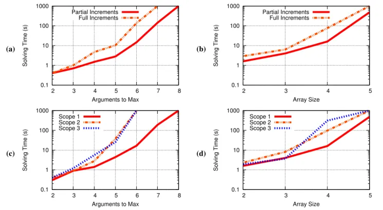
We also used the program synthesis benchmarks to an-swer two questions unique to Alloy*. First, we evaluated the optimization discussed in Section 7.2 by running the bench-marks with and without it. Figures 14(a) and (b) show that
for themaxandarraybenchmarks, respectively, using
first-order increments decreases solving time significantly, and often causes the solver to scale to slightly larger sizes.
Second, we evaluated the benefits to be gained by specify-ing tighter bounds on the problem domain by placspecify-ing tighter limits on the abstract syntax tree nodes considered by the
solver. Figures 14(c) and (d) show that formax andarray
respectively, significant gains can be realized by tightening
the bounds—in the case of max, tighter bounds allow
Al-loy* to improve from solving the 6-argument version of the problem to solving the 8-argument version. For these ex-periments, Scope 1 specifies the exact number of each AST node required; Scope 2 specifies exactly which types of AST nodes are necessary; and Scope 3 specifies only how many total nodes are needed. Other solvers also ask the user to bound the analysis—Sketch, for example, requires both an integer and recursion depth bound—but do not provide the same fine-grained control over the bounds as Alloy*.
Table 1 contains both the running time and the number of candidates considered in solving each benchmark under each of the three scopes discussed above. Because they involve
so few nodes, the bounds for the polybenchmarks could
not be tightened beyond the most general scope. The results for the other benchmarks indicate that carefully considered scopes can result in significantly better solving times (other researchers have also reported similar findings [16]).
These results show that Alloy* not only scales better than naive approaches to program synthesis, but can also, in cer-tain cases, be competitive with state-of-the-art solvers based on years of optimization. Moreover, Alloy* requires only
0.01 0.1 1 10 100 1000
max-2 max-3 max-4 max-5 array-search-2 array-search-3 array-search-4 array-search-5
Solving Time (s) Benchmark Alloy* Enumerative Stochastic Symbolic Sketch
Figure 13. Performance Comparison between Alloy* and
Refer-ence Solvers.
the simple model presented here—which is easier to pro-duce than even the most naive purpose-built solver. Due to its generality, Alloy* is also, in some respects, a more flexi-ble program synthesis tool—it makes it easy, for example, to experiment with the semantics of the target language, while solvers like Sketch have their semantics hard-coded.
Problem Scope 1 Scope 2 Scope 3
Steps Time(ms) Steps Time Steps Time
poly – – – – 2 37 poly-1 – – – – 2 36 poly-2 – – – – 4 281 poly-3 – – – – 3 121 poly-4 – – – – 3 891 max-2 3 311 3 432 3 416 max-3 6 923 7 901 8 1,236 max-4 8 1,536 8 2,983 15 5,928 max-5 25 4,152 23 36,344 19 28,580
max-6 29 16,349 n/a t/o n/a t/o
max-7 44 163,643 n/a t/o n/a t/o
max-8 32 987,345 n/a t/o n/a t/o
array-2 8 1,638 8 2,352 8 1,923
array-3 13 4,023 9 8,129 7 3,581
array-4 15 16,102 11 97,983 15 310,492
array-5 18 485,698 n/a t/o n/a t/o
Table 1. Performance on Synthesis Benchmarks
9. Related Work
The ideas and techniques used in this paper span a number of different areas of research including (1) constraint solvers, (2) synthesizers, (3) program verifiers, and (4) executable specification tools. A brief discussion of how a more pow-erful analysis engine for Alloy (as offered by Alloy*) may affect the plethora of existing tools built on top of Alloy is also in order.
Constraint solvers SMT solvers, by definition, find satis-fying interpretations of first-order formulas over unbounded domains. In that context, only quantifier-free fragments are decidable. Despite that, many solvers (e.g., Z3 [7]) sup-port certain forms of quantification by implementing an
effi-(a) 0.1 1 10 100 1000 2 3 4 5 6 7 8 Solving Time (s) Arguments to Max Partial Increments Full Increments (b) 0.1 1 10 100 1000 2 3 4 5 Solving Time (s) Array Size Partial Increments Full Increments (c) 0.1 1 10 100 1000 2 3 4 5 6 7 8 Solving Time (s) Arguments to Max Scope 1 Scope 2 Scope 3 (d) 0.1 1 10 100 1000 2 3 4 5 Solving Time (s) Array Size Scope 1 Scope 2 Scope 3
Figure 14. Effects of Increment Type and Scope on Solving Time cient matching heuristic based on patterns provided by the
user [6]. Certain non-standard extension allow quantifica-tion over funcquantifica-tions and relaquantifica-tions for the purpose of checking properties over recursive predicates [5]. In the general case, however, this approach often leads to “unknown” being re-turn as the result. Many tools that build on top of an SMT solver raise the level of abstraction of the input language, so that they can provide quantification patterns that work more reliably in practice. For instance, Boogie [4] is an intermedi-ate verification language that effectively uses quantifiers for the task of program verification, but does not allow asser-tions to be higher-order.
SAT solvers, on the other hand, are design to work with bounded domains. Even though they accept only proposi-tional formulas, tools built on top may support richer log-ics, including higher-order quantifiers. One such tool is Kod-kod [38], which, at the language level, allows quantifica-tion over arbitrary relaquantifica-tions. The Kodkod analysis engine, however, is not capable of handling any higher-order formu-las. Rosette [39] builds on top of Kodkod a whole suite of tools for embedding automated constraint solvers into pro-grams for a variety of purposes, including program synthe-sis. Rosette, like many other synthesizers, implements a syn-thesis algorithm internally. In contrast to Alloy*, at the user level, this approach enables only one predetermined form of synthesis (namely, the user specifies a grammar and a prop-erty, and Rosette then finds an instantiation of that grammar satisfying the property).
Synthesizers State-of-the-art synthesizers today are mainly purpose-built. Domains of application include program syn-thesis (e.g., Sketch [36], Storyboard [34], Jennisys [22], Comfusy [19], PINS [37]), automatic grading of program-ming assignments [35], synthesis of data manipulation reg-ular expressions [13], and so on, all using different ways for the user to specify the property to be satisfied. A recent effort has been made to establish a standardized format for pro-gram synthesis problems [3]; this format is syntax-guided, similar to that of Rosette, and thus less general than the for-mat offered by Alloy*. In other words, while each such tool is likely to beat Alloy* in its own concrete domain, it would be hard to apply the tool at all in a different domain. Program Verifiers Program verifiers benefit directly from more expressive specification languages equipped with more powerful analysis tools. In recent years, many efforts have been made towards automatically verifying programs in higher-order languages. Liquid types [30] and HMC [17] respectively adapt known techniques for type inference and abstract interpretation for this task. Bjørner et al. examine direct encodings into Horn clauses, concluding that cur-rent SMT solvers are effective at solving clauses over in-tegers, reals, and arrays, but not necessarily over algebraic datatypes. Dafny [21] is the first SMT-based verifier to pro-vide language-level mechanisms specifically for automating proofs by co-induction [23].
Executable Specifications Many research projects explore the idea of extending a programming language with
sym-bolic constraint-solving features (e.g., [18, 25, 32, 39, 41]). Limited by the underlying constraint solvers, none of these tools can execute a higher-order constraint. In contrast, we used αRby [26] (our most recent take on this idea where we embed the entire Alloy language directly into Ruby), equipped with Alloy* as its engine, to run all our graph ex-periments (where αRby automatically translated input par-tial instances from concrete graphs, as well as solutions re-turned from Alloy back to Ruby objects), demonstrating how a higher-order constraint solver can be practical in this area. Existing Alloy Tools Certain tools built using Alloy al-ready provide means for achieving tasks similar to those we used as Alloy* examples. Aluminum [28], for instance, ex-tends the Alloy Analyzer with a facility for minimizing solu-tions. It does so by using the low-level Kodkod API to selec-tively remove tuples from the resulting tuple set. In our graph examples, we were faced with similar tasks (e.g., minimiz-ing vertex covers), but, in contrast, we used a purely declara-tive constraint to assert that there is no other satisfying solu-tion with fewer tuples. While Aluminum is likely to perform better on this particular task, we showed in this paper (Sec-tion 8.1) that even the most abstract form of specifying such minimization/maximization tasks scales reasonably well.
Rayside et al. used the Alloy Analyzer to synthesize it-erators from abstraction functions [29], as well as com-plex (non-pure) AVL tree operations from abstract specifi-cations [20]. In both cases, they target a very specific cate-gories of programs, and their approach is based on insights that hold only for those particular categories.
10. Conclusion
Software analysis and synthesis tools have typically pro-gressed by the discovery of new algorithmic methods in spe-cialized contexts, and then their subsequent generalization as solutions to more abstract mathematical problems. This trend—evident in the history of dataflow analysis, symbolic evaluation, abstract interpretation, model checking, and con-straint solving—brings many benefits. First, the translation of a class of problems into a single, abstract and general formulation allows researchers to focus more sharply, result-ing in deeper understandresult-ing, cleaner APIs and more efficient algorithms. Second, generalization across multiple domains allows insights to be exploited more widely, and reduces the cost of tool infrastructure through sharing of complex an-alytic components. And third, the identification of a new, reusable tool encourages discovery of new applications.
In this paper, we have argued that the time is ripe to view higher-order constraint solving in this context, and we have proposed a generalization of a variety of algorithms that we believe suggests that the productive path taken by first-order solving might be taken by higher-order solving too. The value of our generalization does not, in our view, rest on its performance in comparison to today’s specialized tools
(although we think it is quite respectable), but instead on the potential for future development of tools that exploit it.
Acknowledgments
This material is based upon work partially supported by the National Science Foundation under Grant No. CCF-1138967.
References
[1] Alloy* Home Page.http://alloy.mit.edu/alloy/hola.
[2] M. Aigner and G. M. Ziegler. Turán’s graph theorem. In Proofs from THE BOOK, pages 183–187. Springer, 2001. [3] R. Alur, R. Bodík, G. Juniwal, M. M. K. Martin,
M. Raghothaman, S. A. Seshia, R. Singh, A. Solar-Lezama, E. Torlak, and A. Udupa. Syntax-guided synthesis. In FM-CAD, pages 1–17. IEEE, 2013.
[4] M. Barnett, B.-Y. E. Chang, R. DeLine, B. Jacobs, and K. R. M. Leino. Boogie: A modular reusable verifier for object-oriented programs. In FMCO 2005, volume 4111 of lncs, pages 364–387. Springer, 2006.
[5] N. Bjørner, K. McMillan, and A. Rybalchenko. Program veri-fication as satisfiability modulo theories. In SMT Workshop at IJCAR, volume 20, 2012.
[6] L. De Moura and N. Bjørner. Efficient e-matching for smt solvers. In Automated Deduction–CADE-21, pages 183–198. Springer, 2007.
[7] L. de Moura and N. Bjørner. Z3: An efficient SMT solver. In TACAS 2008, volume 4963 of lncs, pages 337–340. Springer, 2008.
[8] G. Dennis. A Relational Framework for Bounded Program Verification. PhD thesis, MIT, 2009.
[9] P. Erdos and A. Renyi. On the evolution of random graphs. Mathematical Institute of the Hungarian Academy of Sci-ences, 5: 17-61, 1960.
[10] J. F. Ferreira, A. Mendes, A. Cunha, C. Baquero, P. Silva, L. S. Barbosa, and J. N. Oliveira. Logic training through algorithmic problem solving. In Tools for Teaching Logic, pages 62–69. Springer, 2011.
[11] K. Fisler, S. Krishnamurthi, L. A. Meyerovich, and M. C. Tschantz. Verification and change-impact analysis of access-control policies. In Proceedings of the 27th ICSE, pages 196– 205. ACM, 2005.
[12] J. P. Galeotti, N. Rosner, C. G. López Pombo, and M. F. Frias. Analysis of invariants for efficient bounded verification. In ISSTA, pages 25–36. ACM, 2010.
[13] S. Gulwani, W. R. Harris, and R. Singh. Spreadsheet data manipulation using examples. Commun. ACM, 55(8):97–105, 2012.
[14] G. Hughes and T. Bultan. Automated verification of access control policies using a sat solver. STTT, 10(6):503–520, 2008.
[15] D. Jackson. Software Abstractions: Logic, language, and analysis. MIT Press, 2006.