Decay of correlations and inference in graphical models

Decay of Correlations and Inference in Graphical

Models

by

Sidhant Misra

B.Tech., Electrical Engineering,

Indian Institute of Technology, Kanpur (2008),

SM., Electrical Engineering and Computer Science,

MIT (2011)

Submitted to the Department of Electrical Engineering and

Computer Science

in partial fulfillment of the requirements for the degree of

Doctor of Philosophy

at the

MASSACHUSETTS INSTITUTE OF TECHNOLOGY

September 2014

@

Massachusetts Institute of Technology 2014. All rights reserved.

Author...

Signature redacted

Department of Electrical Engineering and Computer Science

Signature

redacted

Certified by ....

Signature redacted

Accepted by...

I

'6

C)

August 28, 2014

David Gamarnik

Professor

Thesis Supervisor

Leslie A. Kolodziejski

OF TECHNOLOGY

SEP

2

5

201

LIBRARIES

Decay of Correlations and Inference in Graphical Models

by

Sidhant Misra

Submitted to the Department of Electrical Engineering and Computer Science on August 28, 2014, in partial fulfillment of the

requirements for the degree of Doctor of Philosophy

Abstract

We study the decay of correlations property in graphical models and its implications on efficient algorithms for inference in these models. We consider three specific problems: 1) The List Coloring problem on graphs, 2) The MAX-CUT problem on graphs with random edge deletions, and 3) Low Rank Matrix Completion from an incomplete subset of its entries. For each problem, we analyze the conditions under which either spatial or temporal decay of correlations exists and provide approximate inference algorithms in the presence of these conditions. In the course of our study of 2), we also investigate the problem of existence of a giant component in random multipartite graphs with a given degree sequence.

The list coloring problem on a graph

g

is a generalization of the classical graph coloring problem where each vertex is provided with a list of colors. We prove the Strong Spatial Mixing (SSM) property for this model, for arbitrary bounded degree triangle-free graphs. Our results hold for any a > a* whenever the size of the list of each vertex v is at least aA(v)

+

P where A(v) is the degree of vertex v and

#

is a constant that only depends on a. The result is obtained by proving the decay of correlations of marginal probabilities associated with the vertices of the graph measured using a suitably chosen error function. The SSM property allows us to efficiently compute approximate marginal probabilities and approximate log partition function in this model.

Finding a cut of maximum size in a graph is a well-known canonical NP-hard problem in algorithmic complexity theory. We consider a version of random weighted MAX-CUT on graphs with bounded degree d, which we refer to as the thinned MAX-CUT problem, where the weights assigned to the edges are i.i.d. Bernoulli random variables with mean p. We show that thinned MAX-CUT undergoes a

computational hardness phase transition at p = pc = d 11: the thinned MAX-CUT

problem is efficiently solvable when p < pc and is NP-hard when p > pc. We show

that the computational hardness is closely related to the presence of large connected components in the underlying graph.

We consider the problem of reconstructing a low rank matrix M from a subset of its entries Mo. We describe three algorithms, Information Propagation (IP), a sequential decoding algorithm, and two iterative decentralized algorithms named the Vertex Least Squares (VLS), which is same as Alternating Minimization and Edge Least Squares (ELS), which is a message-passing variation of VLS. We provide sufficient conditions on the structure of the revelation graph for IP to succeed and show that when M has rank r = 0(1), this property is satisfied by Erdos-Renyi graphs with edge probability Q ((,g-) 'r). For VLS, we provide sufficient conditions in the special case of positive rank one matrices. For ELS, we provide simulation results which shows that it performs better than VLS both in terms of convergence

speed and sample complexity. Thesis Supervisor: David Gamarnik Title: Professor

Acknowledgments

First and foremost, I am extremely grateful to my advisor, Professor David Gamarnik, for his guidance and support. His patient and systematic approach were critical in helping me navigate my way through the early stages of research. He was very gen-erous with his time; our discussions often lasted more than two hours, where we delved into the finer technical details. I learnt tremendously from our meetings and they left me with renewed enthusiasm. David has also been an extremely supportive mentor, and has offered a lot of encouragement and guidance in my career decisions. I would like to thank my committee members Professor Patrick Jaillet and Pro-fessor Devavrat Shah for offering their time and support. Patrick brought fruitful research opportunities my way, and also gave me the wonderful opportunity to be a part of the Network Science course as a TA with him. Devavrat was kind enough to mentor me in my early days at MIT and introduced me to David. His continued encouragement and his valuable research insights have been incredibly helpful.

My time at MIT would not have been as enjoyable without the many friends and colleagues I met at LIDS. I would like to thank Ying Liu for all his help, the fun chats over lunch, and the topology and algebra study sessions. I would also like to thank my officemates James Saunderson and Matt Johnson for their enjoyable company and many stimulating white board discussions.

This thesis would not have been possible without the support of my parents. Their unconditional love and encouragement has helped me overcome the many challenges I have encountered throughout the course of my PhD, and for that I am eternally grateful. Finally, I am very grateful to Aliaa for being my comfort and home, and for making my journey at MIT a wonderful experience.

Contents

1

Introduction 11

1.1 Graphical Models and Inference ... 11

1.2 Decay of Correlations . . . . 13

1.3 Organization of the thesis and contributions . . . . 15

2 Strong Spatial Mixing for List Coloring of Graphs 27 2.1 Introduction . . . . 27

2.2 Definitions and Main Result ... 30

2.3 Preliminary technical results ... . ... 32

2.4 Proof of Theorem 2.3 ... 38

2.5 Conclusion ... . 49

3 Giant Component in Random Multipartite Graphs with Given De-gree Sequences 51 3.1 Introduction ... 51

3.2 Definitions and preliminary concepts ... ... 55

3.3 Statements of the main results ... 59

3.4 Configuration Model ... 63

Supercritical Case . . . . Size of the Giant Component . . . . ... Subcritical Case . . . . Future Work . . . .. 4 MAX-CUT on Bounded Degree Graphs

tions wi 4.1 Introduction ... 4.2 Main Results ... 4.3 Proof of Theorem 4.1 ... 4.4 Proof of Theorem 4.2 ...

4.4.1 Construction of gadget for reduction 4.4.2 Properties of 7, . . . . 4.4.3 Properties of MAX-CUT on

7 4,

. 4.5 Conclusion . . . .

th Random Edge Dele-99 . . . . 99 ... 102 ... 103 S. . . ... 105 . . . .. . 105 ... 107 . . . 113 . . . 126

5 Algorithms for Low Rank Matrix Completion 5.1 Introduction ...

5.1.1 Formulation . . . ... 5.1.2 Algorithms . . . . 5.2 Information Propagation Algorithm . . . . 5.3 Vertex Least Squares and Edge Least Squares Algorithms . 5.4 Experiments . . . . 5.5 Discussion and Future Directions . . . . 3.6 3.7 3.8 3.9 70 87 94 97 127 127 127 129 130 135 142 144

List of Figures

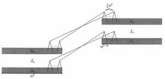
4-1 Illustration of the bipartite graphs J, and J,, in W associated with an

edge (u, v) E C . . . ... . . . 107

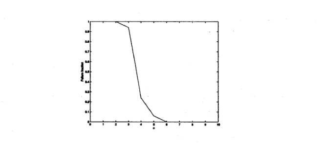
5-1 RMS vs number of iteration (normalized) for VLS and ELS . . . 143 5-2 ELS: Failure fraction vs c for r = 2 with planted 3-regular graph

(n = 100) . . . 145 5-3 ELS: Failure fraction vs c for r = 3 with planted 4-regular graph

(n = 100) . . . 146 5-4 VLS: Failure fraction vs c for r = 2 with planted 3-regular graph

Chapter 1

Introduction

1.1

Graphical Models and Inference

Graphical models represent joint probability distributions with the help of directed or undirected graphs. These models aim at capturing the structure present in the joint distribution, such as conditional independencies, via the structure of the representing graph. By exploiting the structure it is often possible to produce efficient algorithms for performing inference tasks on these models. This has led to graphical models being useful in several applications, e.g., image processing, speech and language processing, error correcting codes, etc.

In this thesis we will be primarily concerned with undirected graphical models, where the joint probability distribution of a set of random variables X1, ... , X, is

represented on an undirected graph

g

= (V, E). The random variables X are asso-ciated with the vertices in V. Undirected graphical models represent independencies via the so-called graph separation property. In particular, let A, B, C C [n] be dis-joint vertices in V. Let XA, XB and Xc denote sub-vectors of X corresponding to

indices in A, B and C respectively. Then XA and XB are independent conditioned on XC whenever there is no path from A to B that does not pass through C, i.e., C separates A and B.

The Hammersely-Clifford theorem [24] says that the joint distribution on g sat-isfies P(x) > 0, then it can be factorized as

P(x) = fl0k(xc), _(1.1)

cEC

where C is the set of all maximal cliques of

g

and Z = E, Ec 0,5(xe) is the normalizing constant, known as the partition function of the distribution.

Broadly speaking, inference in graphical models refers to the following two prob-lems: a) Computation of marginal or conditional marginal probabilities and b)

Com-putation of the Maximum Aposteriori Probability (MAP) assignment. The first

prob-lem involves an integration or counting operation of the form

P(x2) =c(xc). (1.2)

j:Ai eEC

The second problem of computing the MAP assignment is an optimization problem of the form

XMAP = arg max flOc(x). (1.3)

cEC

Both of these problems are typically computationally difficult. In fact, in the general setting, computing MAP assignments is known to be an NP-complete problem and computing marginals is known to be a #P-complete problem. In such cases, it is often desirable to produce approximate solutions in polynomial time by constructing

Polynomial Time Approximation Schemes (PTAS). More precisely, if we denote the quantity of interest, i.e., marginal probabilities or MAP assighments associated with each vertex of a graph on n vertices to be (v), then for a fixed e > 0, a PTAS computes an approximate solution O(v) which is at most a multiplicative factor of (1 E) _{away from 4(v) in time polynomial in n. If the algorithm also takes} time polynomial in 1/c, then it is called a Fully Polynomial Time Approximation Scheme (FPTAS). Approximation algorithms can be either randomized (in which case abbreviations PRAS and FPRAS are commonly used) or deterministic in nature. For some graphical models, it may not be possible to find a PTAS, unless P = NP. There is a substantial body of literature [30], [15], [1]. exploring the existence of PTAS for NP-hard problems.

1.2

Decay of Correlations

The decay of correlations property is a property associated with either the graphical model itself (spatial correlation decay) or an iterative algorithm A that computes the quantity of interest q(v) (temporal or computation tree correlation decay). It describes a long range independence phenomenon, where the dependence on bound-ary/initial conditions fades as one moves away from the boundbound-ary/initial time.

(a) Spatial correlation decay: The impact on 4(v) resulting from conditioning on values of vertices that are at a distance greater than d from v decays as d increases. More precisely, for any vertex v let B(v, d) denote the set of all vertices of G at distance at most d from v. Let x,, and X,2 be two assignments

on X(v,r) . Then

S- c(d) <) < 1 + E(d) (1.4)

-t(V; Xa,₂

)-where E(d) is some decaying function of d that dictates the rate of correlation decay.

(b) Temporal correlation decay: The impact of initial conditions on the quantity

$(v) computed by d iterations of the algorithm A decays as d increases. Similar

to spatial correlation decay, if we denote by xz and

4)

two initial conditions provided to the algorithm A, then temporal decay of correlations refers to the statement for 0(v) analogous to (1.4), i.e.,

o(v; (0))

1-E(d) V < 1+ e(d). (1.5)

The decay of correlations property has its origins in statistical physics, specifi-cally in the study of interacting spin systems. In this context, the spatial decay of correlations property is referred to as spatial mixing where it is used to describe the long range decay of correlations between spins with respect to the Gibbs measure associated with the system. Spatial mixing has its implications on the uniqueness of the so called infinite volume Gibbs measure [13], [21], [49]. The onset of spatial mix-ing is associated with a phase transition from multiple Gibbs measures to a unique Gibbs measure.

On the other hand, temporal decay of correlations is referred to as temporal

mix-ing in statistical physics, where it is most often used to describe the mixmix-ing time

chain on the state space of the spin system whose steady state distribution is the Gibbs measure. Temporal mixing attracted a lot of attention in theoretical computer science, because it can be used to produce approximation schemes based on Markov Chain Monte Carlo (MCMC) methods. Spatial mixing as well has been used to produce approximation schemes which are deterministic in nature and are based on directly exploiting the spatial long range independence. In the context of theoretical computer science, this provides insight into the hardness of algorithmic approxima, tions in several problems. There is a general conjecture that the onset of spatial mixing (phase transition to the unique Gibbs measure regime) coincides with the phase transition in the hardness of approximation. Specifically, the approximation problem is tractable (solvable in polynomial time) if and only if the corresponding Gibbs measure exhibits the decay of correlations property.

1.3

Organization of the thesis and contributions

In this section, we describe the problems we investigate in the thesis, along with a brief survey of the related literature. We state our main results and describe briefly the technical tools we used to establish them. We also state a few relevant open problems.

STRONG SPATIAL MIXING FOR THE LIST COLORING PROBLEM, CHAPTER 2

Formulation

The list coloring problem is a generalization of the classical graph coloring problem. In the list coloring problem on a graph g = (V, C), with maximum degree A, each

{1, 2, ... q}, where {1, 2,.. , q} is the superset of all colors. In a valid coloring, each vertex is assigned a color from its own list such that no two neighbors in g are assigned the same color. It is well known that in this general setting, deciding whether a valid coloring exists is NP-hard and counting the number of proper colorings is #P-hard.

One can associate a natural graphical model with the list coloring problem which represent the uniform distribution on the space of all valid colorings. The partition function of this graphical model is the total number of valid colorings. As mentioned earlier, computing the partition function, and hence performing the inference task of computing the marginal probabilities exactly is computationally intractable. There is a large body of literature describing randomized approximation schemes to com-pute marginal probabilities and the number of valid colorings based on a Markov Chain Monte Carlo (MCMC) method. Most results are based on establishing fast mixing of the underlying Markov chain known as the Glauber Dynamics [31], [261, [51], [42]. Deterministic approximation schemes based on decay of correlations in the computation tree have also been studied in the literature [18]. These results are es-tablished with an assumption on the relation between the number of colors available and the degree, i.e.,

ILI

> aA + #. Over time, considerable research effort has been directed towards relaxing the assumption by decreasing the value of a required in the aforementioned condition. In fact, it is known for the special case of A-regular trees that spatial decay of correlations exists as early as a = 1 and 8 = 2, which also marks the boundary of phase transition into the unique Gibbs measure regime. It is conjectured that a = 1 and 6 = 2 is sufficient for existence of spatial decay of correlations and existence of approximation algorithms in the list coloring problem.

Contributions

cor-relations called Strong Spatial Mixing (SSM) for the list coloring problem whenever a > a* ; 1.76. Ours is the most general conditions under which strong spatial mix-ing has been shown to exist in the literature, and is a step towards establishmix-ing SSM for a = 1 as conjectured. As a corolary of our result, we also establish the uniqueness of Gibbs measure for the list coloring problem and the existence of approximation schemes for computing marginal probabilities in this regime.

Our proof technique has two main components. The first component is a recur-sion we derive that relates the marginal probabilities at a vertex to the marginal probabilities of its neighbors. This recursion is a variation of the one derived in [18] where our recursion deals with the ratio of marginals rather than directly with the marginals themselves. The second component is the construction of an error func-tion which is chosen suitably such that it interacts well with our recursion. To prove our result, we then show that the distance between two marginals induced by two different boundary conditions satisfies a certain contraction property with respect to the error function.

Open Problems

There are several problems still to be addressed. One is to tighten our result and establish SSM for a = 1 and 6 = 2 as conjectured. Second, the SSM result we es-tablish, allows the construction of a PTAS for computing marginal probabilities, and computing the exponent of the partition function up to a constant factor. However, it does not directly lead to an FTPAS for the partition function. It is still unresolved whether SSM by itself is sufficient for constructing FPTAS.

GIANT COMPONENT IN RANDOM MULTIPARTITE GRAPHS, CHAP-TER 3

Formulation

The problem of the existence of a giant component in random graphs was first stud-ied by Erdos and R6nyi. In their classical paper [16], they considered a random graph model on n and m edges where each such possible graph is equally likely. They showed that if m/n > 1 + c, then with high probability as n -+ oo, there exists a component of size linear in n in the random graph and that the size of this component as a fraction of n converges to a fixed constant. The degree distribution of the classical Erd6s-R6nyi random graph has asymptotically Poisson degree dis-tribution. However in many applications the degree distribution associated with an underlying graph does not satisfy this property. For example, many so-called "scale-free" networks exhibit power law distribution of degrees. This motivated the study of random graphs generated according to a given degree sequence. The giant com-ponent problem on a random graph generated according to a given degree sequence was considered by Molloy and Reed [43]. They showed that if a random graph has asymptotic degree sequence given by {pj}L1, then with high probability it has a

giant component whenever the degree sequence satisfies 'jj(j - 2)p > 0, along with some additional regularity conditions including the bounded second moment condition. A key concept in their proof was the construction of the so called

explo-ration process which reveals the random component of a vertex sequentially. They

showed that whenever the degree sequence satisfies the aforementioned condition, the exploration process has a strictly positive initial drift, which when combined with the regularity conditions is sufficient to prove that at least one of the components must be of linear size. They also show that there is no giant component whenever

{IM!, < 0 and in [44] also characterize the size of the giant component. Since

then, there has been several papers strengthening the results of Molloy and Reed and several beautiful analysis tools have been invented along the way. We defer a more detailed literature review to Chapter 3. We mention here a relatively recent paper by Bollobas and Riordan [81, where they use a branching process based analy-sis that offers several advantages, including tighter probability bounds and relaxing the finite second moment assumption.

In this thesis, we study random multipartite graphs with p parts with given de-gree distributions. Here p is a fixed positive integer. Each vertex is associated with a degree vector d, where each of its component di, i E [p] dictates the number of neighbors of the vertex in the corresponding part i of the graph. Several real world networks naturally demonstrate a multipartite nature. The author-paper network, actor-movie network, the network of company ownership, the financial contagion model, heterogenous social networks, etc. are all multipartite

[46],

[9], [27 in na-ture. Examples of biological networks which exhibit multipartite structure include drug target networks, protein-protein interaction networks and human disease net-works [22], [56], [45. In many cases evidence suggests that explicitly modeling the multipartite structure results in more accurate models and predictions.

We initiated our study of the giant component problem in multipartite graphs because it was needed as a part of the proof of our hardness result in Chapter 4 for the MAX-CUT with edge deletions problem. However, the problem of giant compo-nent is also of independent interest and we devote a whole chapter to it.

Contributions

We provide exact conditions on the degree distribution for the existence of a giant component in random multipartite graphs with high probability. In the case where

a giant component exists, we also provide a characterization of its size in terms of parameters of the degree distribution.

Our proofs involve a blend of techniques from Molloy and Reed [43] and Bollobas and Riordan [8] along with results from the theory of multidimensional branching processes. We show that whenever the matrix of means M of the so called edge-biased degree distribution satisfies the strong connectivity property, then the existence of a giant component is governed by the Perron-Frobenius eigenvalue Am of M. Whenever

AM > 1, we show that a certain Lyapunov function associated with the exploration process of Molloy and Reed has a strictly positive drift. The Lyapunov function

we use is one often used in the analysis of multi type branching processes, which is a weighted f, norm Lyapunov function constructed by using the Perron-Frobenius eigenvector of M. To establish results regarding the size of the giant component, we use a coupling argument relating from Bollobas and Riordan [8], relating the explo-ration process to the multi type branching process associated with the edge-biased degree distribution.

Open Problems

Our result only addresses the super-critical and sub-critical case, but leaves the critical case unresolved. This has been studied in detail for random graphs with degree distributions for the uni-partite case [34]. It may be possible to extend these results to the multipartite case as well.

MAX-CUT ON GRAPHS WITH RANDOM EDGE DELETIONS, CHAP-TER 4

Formulation

The problem of finding a cut of maximum size in an arbitrary graph g = (V, C) is a

well known NP-hard problem in algorithmic complexity theory. In fact, even when restricted to the set of 3-regular graphs, MAX-CUT is NP-hard with a constant factor approximability gap [5], i.e., it is NP-hard to find a cut whose size is at least (1- Ec,.itia) times the size of the maximum cut, where c ,.mg = 0.997. The weighted MAX-CUT is a generalization of the MAX-CUT problem, where each edge e E E is associated with a weight we, and one is required to find a cut such that the sum of the weights of the edges in the cut is maximum.

We study a randomized version of the weighted MAX-CUT problem, where each weight W is a Ber(p) random variable, for some 0 5 p < 1, and the weights asso-ciated with distinct edges are independent. Since the weights are binary, weighted MAX-CUT on the randomly weighted graph is equivalent to MAX-CUT on a thinned random graph where the edges associated with zero weights have been deleted. We call this problem the thinned MAX-CUT. The variable p controls the amount of thinning. It is particularly simple to analyze thinned MAX-CUT, when p takes one of the extreme values, i.e., p = 1 and p = 0. When p = 1, all edges are retained and the thinned graph is same as the original graph and finding the maximum cut remains computationally hard. On the other hand, when p = 0, the thinned graph has no edges, and the MAX-CUT problem is trivial. This leads to a natural question of whether there is a hardness phase transition at some value of 0 < p = pc < 1.

Our study of the thinned MAX-CUT problem is motivated from the point of view of establishing a correspondence between phase transition in hardness of computation

and decay of correlations. Our formulation of the thinned MAX-CUT problem was inspired by a similar random weighted maximum independent set problem studied by Gamarnik et. al in [19].

Contributions

We identify a threshold for hardness phase transition in the thinned MAX-CUT problem. We show that on the set of all graphs with degree at most d, the phase transition occurs at p, = d_1. We show that this phase transition coincides with a phase transition in decay in correlations resulting from the connectivity properties of the random thinned graph. This result is a step towards showing the equivalence of spatial mixing and hardness of computation.

For p < pc we show that the random graph resulting from edge deletions un-dergoes percolation, i.e., it disintegrates into disjoint connected components of size

O(log n). The existence of a polynomial time algorithm to compute MAX-CUT then

follows easily. For p > pc, we show NP-hardness by constructing a reduction from

approximate MAX-CUT on 3-regular graphs. Our reduction proof uses the

ran-dom bipartite graph based gadget W similar to [501, where it was used to establish hardness of computation of the partition function of the hardcore model. Given a 3-regular graph

g,

the gadget W is d-regular and is constructed by first replacing each vertex v of

g

by a random bipartite graph J, of size 2n' consisting of two parts

R, and S, and then adding connector edges between each pair of these bipartite

graphs whenever there is an edge between the corresponding vertices in

g.

The key result in our reduction argument is that the gadget W satisfies a certain polarization

property which carries information about the MAX-CUT on the 3-regular graph

g

used to construct it. Namely, we show that any maximal cut of the thinned graph

-,

obtained from W must fully polarize each bipartite graph and include all its edges

in the cut, i.e., either assign the value 1 to almost all vertices in R, and 0 to almost all vertices in S, or vice versa. Then, we show that the cut Cg of g obtained by assigned binary values to its vertices v based on the polarity of J, must be at least (1 - ec,.tes)-optimal. To establish this polarization property we draw heavily on the results and proof techniques from Chapter 3 about the giant component on random multipartite graphs.

Open Problems

While our result finds the exact hardness phase transition threshold for the thinned MAX-CUT problem, the same remains unresolved for the thinned maximum indepen-dent set problem in [19] from which our problem was originally inspired. There, only half of the result has been established, as in the region where decay of correlations and an approximate algorithm exists has been identified. It remains open whether in the absence of decay of correlations, computing the maximum independent set is computationally hard.

ALGORITHMS FOR LOW RANK MATRIX COMPLETION, CHAP-TER 5

Formulation

Matrix completion refers to the problem of recovering a low rank matrix from a sub-set of its entries. This problem arises in a vast number of applications that involve

collaborative filtering, where one attempts to predict the unknown preferences of a

certain user based on collective known preferences or a large number of users. It attracted a lot of attention due to the famous Netfliz prize, which involved recon-structing the unknown movie preferences of Netflix users.

In matrix completion, there is an underlying low rank matrix M E R" of rank

r < n , i.e., M = a)' where a, P

E

Rn"x. The value of the entires of M on a subset a indices S C [n] x [n] is revealed. Denoting by Mg the subset of revealed entries of

M, the two major questions of matrix completion are:

(a) Given Mo, is it possible to reconstruct M? (b) Can the reconstruction in (a) be done efficiently?

Without any further assumptions, matrix completion is an ill posed problem with multiple solutions and is in general NP-hard [41]. However under certain additional conditions, the problem has been shown to be tractable. The most common assump-tion adopted in the literature is that the matrix M is "incoherent" and the subset

E is chosen uniformly at random. The incoherence condition was introduced in [10],

[11}, ivhere it was shown that convex relaxation resulting in nuclear norm minimiza-tion succeeds with further assumpminimiza-tions on the size of E. In [35] and [361, the authors use an algorithm consisting of a truncated singular value projection followed by a local minimization subroutine on the Grassmann manifold and show that it succeeds when JE == (nr log n). In [28], it was shown that the local minimization in [35] can

be successfully replaced by Alternating Minimization. The use of Belief Propagation (BP) for matrix factorization has also been studied by physicists in [33] heuristically, where they perform a mean field analysis on the performance of BP.

Matrix completion can be recast as a bi-convex least squares optimization prob-lem over a graph

g

= (V, 6) whose edges represent the revealed entries of M. On

this graph, Alternating Minimization can be interpreted as a local algorithm, where the optimization variables are associated with the vertices V. In each iteration, the variable on a vertex is updates using the value of its neighbors. Since in [28], Al-ternating Minimization is preceded by a Singular Value Projection (SVP), we call it

a warm-start Alternating Minimization. In this thesis, we investigate, Alternating Minimization, which we call Vertex Least Squares (VLS), when it is used with a cold start. We also propose two new matrix completion algorithms.

Contributions

We analyze VLS with a cold start and prove that in the special case of positive rank one matrices, it can successfully reconstruct M from Mg. More specifically, we show that if M = af' with a,# > 0 and the graph G is connected, has bounded degree and diameter of size O(log n), then VLS reconstructs M up to a Root Mean Square (RMS) error of e in time polynomial in n.

We propose a new matrix completion algorithm called Edge Least Squares (ELS), which is a message passing variation of VLS. We show through simulations that ELS performs significantly better than VLS, both in terms of sample complexity and time till convergence. The superior cold start performance of ELS suggests that ELS with warm start can be perhaps very successful, and would be better than VLS with warm start.

We also provide a simple direct decoding algorithm, which we call Information Propagation (IP). We prove that under certain strong connectivity properties of g,

Information Propagation can recover M in linear time. We show that when r = 0(1),

the required strong connectivity property satisfied by a bipartite Erdos-Renyi graph g(n,p) with p = Q ((In)1/r)

Open Problems

It remains an open problem to provide a theoretical analysis to prove the convergence of ELS. The full power of cold start VLS is also unresolved and it may be possible to extend our proof for the rank one case to the higher rank case. Additionally, it may

be possible to provide theoretical analysis to demonstrate the superior performance of ELS over VLS.

Chapter 2

Strong Spatial Mixing for List

Coloring of Graphs

2.1

Introduction

In this chapter we study the problem of list colorings of a graph. We explore the strong spatial mixing property of list colorings on triangle-free graphs which per-tains to exponential decay of boundary effects when the list coloring is generated uniformly at random from the space of valid list-colorings. This means fixing the color of vertices far away from a vertex v has negligible impact (exponentially decay-ing correlations) on the probability of v bedecay-ing colored with a certain color in its list. Strong spatial mixing is an instance of the spatial decay of correlations property. A related but weaker notion is weak spatial mixing. Strong spatial mixing is stronger than weak spatial mixing because it requires exponential decay of boundary effects even when some of the vertices near v are conditioned to have fixed colors. Because of this added condition, strong spatial mixing is particularly useful in computing

conditional marginal probabilities.

Jonasson in [32] established weak spatial mixing on Kelly (regular) trees of any degree A whenever the number of colors q is greater than or equal to A +1. How-ever the weakest conditions for which strong spatial mixing on Kelly trees has been established thus far is by Ge and Stefankovic [20] who proved strong spatial mixing when q

>

a*A + 1, where a* = 1.763.. is the unique solution to xe 1 1 = 1. For lat-tice graphs (or more generally triangle-free amenable graphs) strong spatial mixing for coloring was established by Goldberg, Martin and Paterson in [23] for the case

q > a*A - 3 for a fixed constant P. In fact their approach can be extended to the case of list coloring problem, but the graph amenability restriction still applies.

In this chapter we generalize these results under only mildly stronger condition. We establish the strong spatial mixing of list colorings on arbitrary bounded degree triangle free graphs whenever the size of the list of each vertex v is at least aA(v) +#,

where A(v) is the degree of v, a satisfies a > a* and

/

is a constant that only depends on a.

The spatial mixing property is closely related to uniqueness of the infinite volume Gibbs measure on the spin system defined by the list coloring problem. In fact weak spatial mixing is a sufficient condition for the Gibbs measure to be unique. In its turn, strong spatial mixing is closely related to the problem of approximately counting the number of valid colorings of a graph, namely the partition function of the Gibbs measure. In particular, for amenable graphs strong spatial mixing implies rapid mixing of Glauber dynamics which leads to efficient randomized approximation algorithms for computing the partition functions, e.g. in [31}, [26], [51], [42] etc. The decay of correlations property similar to strong spatial mixing has also been shown to lead to deterministic approximation algorithms for computing the partition functions. This technique was introduced by Bandyopadhyay and Gamarnik [3]

and Weitz [53] and has been subsequently employed by Gamarnik and Katz [18} for the list coloring problem. Since decay of correlations implies the uniqueness of Gibbs measure on regular trees and regular trees represent maximal growth of the size of the neighborhood for a given degree, it is a general conjecture that efficient approximability of the counting problem coincides with the uniqueness of Gibbs measure on regular trees. More precisely the conjecture states that there exists a polynomial time approximation algorithm for counting colorings of any arbitrary graph, whenever q > A + 2. We are still very far from proving this conjecture or even establishing strong spatial mixing under this condition.

The formulation in this chapter is similar to [18] . It was shown there that the logarithm of the ratio of the marginal probabilities at a given node induced by the two different boundary conditions contract in fe, norm as distance between the node and the boundary becomes large, whenever IL(v)I > aA(v)+#8, and a > a** ; 2.78..

and 8 is a constant that only depends on a. In this chapter we measure the distance with respect to a conveniently chosen error function which allows us to tighten the contraction argument-and relax the required condition to a > a* ; 1.76... This also means that the Gibbs measure on such graphs is unique. Unlike [181 the result presented in this chapter unfortunately does not immediately lead to an algorithm for computing the partition function. It does however allow us to compute the marginal probabilities approximately in polynomial time. It also allows us to estimate the exponent of the number of valid colorings, namely apprximate the log-partition function in polynomial time.

The rest of the chapter is organized as follows. In Section 3.2 we introduce the notation, basic definitions and preliminary concepts. Also in this section we provide the statement of our main result and discuss in detail its implications and connections to previous results. In Section 2.3 we establish some preliminary technical results.

In Section 2.4 we prove our main result of this chapter. We conclude in Section 2.5 with some final remarks.

2.2

Definitions and Main Result

We denote by

g

= (V, E) an infinite graph with the set of vertices and edges given

by V and E. For a fixed vertex v E V we denote by A(v) the degree of v and by A the maximum degree of the graph, i.e. A = maxEv A(v) < oo. The distance between two vertices v, and v2 in V is denoted by d(vi, v2) which might be infinite if

v, and v2 belong to two different connected components of g. For two finite subsets

of vertices 1_{I c V and '2 C V, the distance between them is defined as d(T1, 2) =}

min{d(vi, v2) : 1 E I1, v2 E F2}. We assume {1, 2, ... , q} to be the set of all colors. Each vertex v E V is associated with a finite list of colors L(v)

c

{1, 2,..., q} and

C = (L(v) : v E V) is the sequence of lists. The total variational distance between

two discrete measures p, and L2 on a finite or countable sample space Q is given by || - A2II and is defined as |tiJ - 121 =ZWEn 'I,.pi(W) - p2(U)|.

A valid list coloring C of g is an assignment to each vertex v E V, a color

c(v) E L(v) such that no two adjacent vertices have the same color. A measure y

on the set of all valid colorings of an infinite graph g is called an infinite volume Gibbs measure with the uniform specification if, for any finite region IF ;

g,

the distribution induced on T by p conditioned on any coloring C of the vertices V\T is the uniform conditional distribution on the set of all valid colorings of T. We denote this distribution by M4. For any finite subset T C g, let

aT

denote the boundary of T, i.e. the set of vertices which are adjacent to some vertex in IF but are not a part of T.

Definition 2.1. The infinite volume Gibbs measure 1A on ! is said to have strong spatial mixing (with exponentially decaying correlations) if there exists positive con-stants A and 0 such that for any finite region T C 9, any two partial colorings C1, C2 (i.e. vertices to which no color has been assigned are also allowed) of V\* which differ only on a subset W C 8, and any subset A C 417

I - A2I < AAje~ (2.1)

Here |yIli - pIC2A denotes the total variational distance between the two distribu-tions y and pf2 restricted to the set A.

We have used the definition of strong spatial mixing from Weitz's PhD thesis [52]. As mentioned in [521, this definition of strong spatial mixing is appropriate for general graphs. A similar definition is used in [23], where the set W of disagreement was restricted to be a single vertex. This definition is more relevant in the context of lattice graphs (or more generally amenable graphs), where the neighborhood of a vertex grows slowly with distance from the vertex. In that context, the definition involving one vertex disagreement and the one we have adopted are essentially the same.

Let a* = 1.76.. be the unique root of the equation

1

e- =

1.

For our purposes we will assume that the graph list pair (9, C) satisfies the following.

satisfies

IL(v)I

> aA(v) + 0. (2.2)

for some constant a > a* and 6 = /8(a) ;

4

is such that

(1 - 1//3)ae-(1+1/)>1

Using the above assumption we now state our main result.

Theorem 2.1. Suppose Assumption 3.1 holds for the graph list pair (G, ). Then the Gibbs measure with the uniform specification on (G, ) satisfies strong spatial mixing with exponentially decaying correlations.

We establish some useful technical results in the next section before presenting the details of the proof in Section (2.4).

2.3

Preliminary technical results

The following theorem establishes strong spatial mixing for the special case when A consists of a single vertex.

Theorem 2.2. Let q, A, a and

3

be given. There exists positive constants B and y depending only on the preceding parameters such that the following holds for any graph list pair (G, ) satisfying Assumption 3.1. Given any finite region T C g, any two colorings C1, C2 of V\T which differ only on a subset W C OT, and any vertex

v E T and color j E L(v), we have

(1-) <P(c(v) _P(c(V) = jCi)_-

_I

_{< < (1 + E) (2.3)} ~P(C(V) = jIC2)

where e = Be-d(W)

We will now show that Theorem 2.1 follows from Theorem 2.2.

Proof of Theorem 2.1. To prove this, we use induction on the size of the subset A.

The base case with JAI = 1 is equivalent to the statement of Theorem 2.2. Assume that the statement of Theorem 2.1 is true whenever JAI t for some integer t

>

1. We will use this to prove that the statement holds when JAI = t + 1. Let the

vertices in A be v,v2,..., vt+1. Let vk = (v1,. .. ,vk) and Jk = (ji,..., jk) where

j E L(vi), 1 < i < k. Also let c(vk) = (c(vi), c(v2),..., c(vk)) denote the coloring of

the vertices v1,V2,... Vk.

P(c(vt+₁) = Jt+1 C1) =P(c(vt) = JtlC)P(c(vt+i = it+i)Ic(vt) = Jt, C1)

<(1 + E)P(C(Vt) = JtIC1)P(c(Vt+ = jt+l)fc(vt) = Jt, C2).

The inequality in the last statement follows from Theorem 2.2. This gives P(c(vt+i) = Jt+|C1) - P(c(vt+i) = 4 C+1C2)

(1

+

E)P(c(vt) = JtIC)P(c(vt+1 = jt+1)IC(vt) = Jt, C2) -P(c(vt) = JtIC2)P(C(Vt+l = jt+l)fc(vt) = Jt, C2)

=EP(c(vt) = JtIC)P(c(Vt+l = jt+l)c(vt) = Jt, C2)

)}-Similarly,

P(c(vt+i) = Jt+I jC1) - P(c(vt+i) = Jt+1 jC2)

>- EP(c(vt) = JtIC1)P(c(Vt+1 = jt+I)Ic(vt) = Jt, C2)

+P(c(Vt+1 = it+I)Ic(vt) = Jt, C2){P(c(vt) = JtIC1) - P(C(vt) = JtIC2

)}-Combining the above, we get

IP(c(vt+I) = Jt+1 C1) - P(c(vt+i) = Jt+11C2)l

eP(C(V) = JttC1)P(c(vt+i = jt+1)jc(vt) = Jt, C2)

+P(c(vt+i = jt+1) c(v) = Jt, C2) I{P(c(vt) = JtICI) - P(c(vt) = JtIC2

)}I-We can now bound the total variational distance lIpIl - p211A as follows.

P(c(vt+i) = Jt+1IC) - P(c(vt+i) = Jt+1IC2)1

jiEL(vi), 1 itt+1

EP(c(vt) = JtIC1)P(c(Vt+l = jit+) Ic(vt) J, C2)

jiEL(v,), 1 i:t+1

+ P(c(t+ =jt+1)Ic(vt) = J, C2) jiEL(vj), 1<iit+1

x

I{P(c(vt)

= JtICi) - P(c(vt) = JtIC₂)}|

whret e

+ n f f|m t i o hs (t +cp)e

where the last statement follows from the induction hypothesis. This completes the

induction argument. 0

true. We claim that Theorem 2.2 follows from the theorem below which establishes weak spatial mixing whenever Assumption 3.1 holds. In other words under Assump-tion 3.1, strong spatial mixing of list colorings for marginals of a single vertex holds whenever weak spatial mixing holds. In fact g need not be triangle-free for this implication to be true as will be clear from the proof below.

Theorem 2.3. Let q, A, a and P be given. There exists positive constants B and

-y depending only on the preceding parameters such that the following holds for any graph list pair (9, L) satisfying Assumption 3.1. Given any finite region T C g, any

two colorings C1, C2 of V\'I, we have

P(c(v) =jjCi)

(1 P(c(v) =

jC)

< (1+ e) (2.4)

P(C(V) = jjC2)

where c = Be - ,aO)

We first show how Theorem 2.2 follows from Theorem 2.3.

Proof of Theorem 2.2. Consider two colorings C1, C2 of the boundary c9i of I which

differ only on a subset W C ft as in the statement of Theorem 2.2. Let d = d(v, W).

We first construct a new graph list pair (a', C') from (g, L). Here g' is obtained from

G by deleting all vertices in OT which are at a distance less than d from v. Notice

that for all such vertices C1 and C2 agree. Whenever a vertex u is deleted from g,

remove from the lists of the neighbors of u the color c(u) which is the color of u under both C1 and C2. This defines the new list L'. In this process, whenever a vertex u loses a color in its list it also loses one of its edges. Also for a > a* > 1, we have

IL(v)| -1 > a(A(v) - 1)+,8 whenever IL(v)| > aA(v)

+fl.

_{Therefore, the new graph}

of radius (d -1) centered at v. Let Di and D2 be two colorings of (V)c which agree with C1 and C2 respectively. From the way in which g', ' is constructed we have

Pg,4C(c(v) = jjCj) = Pg,,,C(c(v) = j|D), for i = 1, 2. (2.5)

where Pg, (E) denotes the probability of the event E in the graph list pair (G).

If V' is the set of all vertices of

g',

then D, and D2 assign colors only to vertices in V'\v. So we can apply Theorem 2.3 for the region V' and the proof is complete. L

So it is sufficient to prove Theorem 2.3 which we defer till section (2.4). We use the rest of this section to discuss some implications of our result and connections between our result and previous established results for strong spatial mixing for coloring of graphs.

The statement in Theorem 2.3 is what is referred to as weak spatial mixing [521. In general weak spatial mixing is a weaker condition and does not imply strong spatial mixing. This is indeed the case when we consider the coloring problem of a graph

g

by q colors, i.e. the case when the lists L(v) are the same for all v E V. However, interestingly, as the above argument shows, for the case of list coloring strong spatial mixing follows from weak spatial mixing when the graph list pair satisfies Assumption 3.1.

We observed that the strong spatial mixing result for amenable graphs in [23] also extends to the case of list colorings. Indeed the proof technique only requires a local condition similar to that in Assumption 3.1 that we have adopted as opposed to a global condition like q ;> aA + P. Also in [23], the factor JAI in the definition (2.1) was shown to be not necessary which makes their statement stronger. We show that this stronger statement is also implied by our result. In particular, assuming Theorem 2.2 is true, we prove the following corollary.

Corollary 2.1. Let q, A, a and ft be given. There exists positive constants B and -y depending only on the preceding parameters such that the following holds for any graph list pair (9,,C) satisfying Assumption 3.1. Given any finite region T C !, any two colorings C1, C2 of the boundary ni of T which differ at only one point f E ft,

and any subset A C xF,

| JAI- pIC211A ; Be --d(Af), _(2.6)

Proof. Let the color of

f

be ji in C1 and j2 in C2. Let C(A) be the set of all possible colorings of the set A.

- p421A = ~

IP(u(f) = ji)

- P(alc(f) =

j2)1

oEC(A)

P(c(f)= _{jila) P(c(f)}

= j210) j

EC(h P2 ji) P(C(f) = 2

For any j E _{L(f), using Theorem 2.2 we have for E = Be-"Yd(Af),}

P(c(f)

=

ijo-)

P(c(f)

=

jla)

P(c(f) = j) E,'EC(A) P(c(f) =

ijl')P(')

ZO!'EC(A) P(c(f) = jjAO)P(u')

YX'Ec(A) P(c(f) =

jlo')P(c')

< EOEC(A) P(c(f) =

il')(1

+ e)P(o') EEC(A) P(Cf) = jj)P()

Similarly we can also prove for any j E L(f) P(c(f) =lo 1-) P(c(f) =

j)

Therefore, pJC - p 21A < (+

f)

- 1 )[P(u-) = 2f. orEC(A)

The notion of strong spatial mixing we have adopted also implies the uniqueness of Gibbs measure on the spin system described by the list coloring problem. In fact

Weak Spatial Miung described in Theorem 2.3 is sufficient for the uniqueness of

Gibbs measure (see Theorem 2.2 and the discussion following Definition 2.3 in [52]). We summarize this in the corollary that follows.

Corollary 2.2. Suppose the graph list pair g, L satisfy Assumption 3. 1. Then the infinite volume Gibbs measure on the list colorings of G is unique.

2.4

Proof of Theorem 2.3

Let v E V be a fixed vertex of

g.

Let m = A(v) denote the degree of v and let

Vi , v2, ... , m be the neighbors of v. The statement of the theorem is trivial if m = 0

(v is an isolated vertex). Let q, =

IL(v)I

and q,,,= L(vi)1. Also let

g,

be the graph obtained from

g

by deleting the vertex v. We begin by proving two useful recursions on the marginal probabilities in the following lemmas.

Lemma 2.1. Let j1, j2

E L(v). Let

4

j,3j denote the list associated with graph ~g

which is obtained from C by removing the color j, from the lists L(vk) for k < i and removing the color j2 from the lists L(vk) for k > i (if any of these lists do not contain the respective color then no change is made to them). Then we have

Pgc(c(v) = ji) m 1 - Pg.,L,, 2 (c(vi) = ji)

PgX-(c(v) =

j

2) j= - P9.,L,,j, (c(vi) = 32)'

Proof Let Zge(M) denote the number of colorings of a finite graph g with the

condition M satisfied. For example, Zgc(c(v) = j) denotes the number of valid

colorings of g when the color of v is fixed to be j E L(v). We use a telescoping product argument to prove the lemma:

Pg C(c(v) = ji) Zg"c(c(v) = ji) PgC(c(v) = j2) ZgX(c(v) = 32)

Zg~,c(c(vi) # ji, 1 <i < M)

Zg,,(C(Vi) 9k j2, 1 <- < M m) Pgg(c(vi)

#

ji

1 K i < m) Pg4X(c(vi) #?2, 1< i <iM) M Pg,,g(c(vk)

0

j1, 1 < k < i, c(vk) 34 j2, i +l 5k 5m) Pg,(c(vk) = ji, 1 k < i - 1, c(v) j2, i<k<m) Pg, L,,(C() 0 2i c(v)

Oi,

k <

1,

C(vk) j2,

i+

<k<m)

P9,,(c(0 )A j 2 jC(vk) 54j,17 < k < 1, c(vk) =A j2, i+ < k< m) M1 -Pg,,-14 (c(vi) = ji) 1 -Pg,,(C(Vi) = j2) 01

The following lemma was proved in [181. We provide the proof here for complete-ness.

Lemma 2.2. Let j E L(v). Let Ci denote the list associated with the graph G,

which is obtained from C by removing the color j (if it exists) from the list L(Vk) for k < i. Then we have ]., (1 - Pg,,r (c(vi) =

j)

Pg C(c(v) = () EkEL(v) M, ~g.,c, (c0e = k)) Proof. Pg C(c(v) =

j)

ZgC(c(v) = j) ZkEL(v) ZgC(c(v) = k) Zg,,t(c(V ) /- j, 1 < i < M)

XIEL(.) Zg.,e(c(vi)

A

k, 1 <i m) Pg,,i(c( ) = A

, 1

< i < m)

kEv)Pgi,,tc(c(vi) =, k, 1 < i < m) Now for any k E L(v),

Pg,c(c(v) 4 k, 1 < i < m) Pg,,,c(c(vi)

$

k) fPg,,c(c(vi) = kjc(vj k, 1 < 1 < k - 1) i=2

Pg,,,4 , (c(v ) k).

Substituting this into (2.7) completes the proof of the lemma. 0

Before proceeding to the proof of Theorem 2.3, we first establish upper and lower bounds on the marginal probabilities associated with vertex v.

Lemma 2.3. Let v

E

T be such that d(v, &F) > 2. For every j

E

L(v) and for

1 = 1, 2 the following bounds hold.

P(c(v) = jIC) < 1/a. (2.8)

P(c(v) = jc) (mae (2.9)

P(c(v) = jC) > q~1_{(1 -}

₁₎

_(2.10)

Here q is the total number of possible colors.

Proof. These bounds were proved in [18] with a different constant, i.e. a > a** :::

2.84. Here we prove the bound when Assumption 3.1 holds. In this proof we assume I = 1. The case 1 = 2 follows by an identical argument. Let C denote the set of all possible colorings of the children v,... ,Vm _{of v. Note that for any c E C,}

P(c(v) = jic) I5 1/1. and (2.8) follows.

To prove (2.9) we will show that for every coloring of the neighbors of the neigh-bors of v, the bound is satisfied. So, first fix a coloring c of the vertices at distance two from v. Conditioned on this coloring, define for j E L(v) the marginal

tij = Pg.,, (c(vi) =

ic).

Note that by (2.8) we have t,, 1/8. Because. is triangle-free, there are no edges between the neighbors of v and once we condition on c, we have

So we obtain

zt

=

jEL(v)

z

Pg,,(c(vi)

=

jic)

<

1. jEL(v)(lL(vj)

From Lemma 2.2 we have

=k]Lv

n(1

- tik)

EkEL(v) M (1- ik)

Using Taylor expansion for log(1 - x), we obtain

(1

- tik) =

I

eIog(1-'-k) e ~2(e i=1 i=1 where 0 ik < tik. So 9 ik satisfies (1 - 0, )2 > (1 1/p)2 > 1/2 by Assumption 3.1. Thus, we obtain

1(1

- t ) e-(1+1/.)tk - / E i1 i=1.

Using the fact that arithmetic mean is greater than geometric mean and using (2.11), we get

[J(1 - tik)

kEL(v) i=1

> qv (1 - tik)

(kEL(v) i=1

> qexp -q,~1(l

_{+ 1/0)E}

_ti,k

i=1 kEL(v) >M > (am+ #)e-(1+1/h6)Q.-> ame-(1+1/,6)Q. P(c(v) = j|C1) (2.11) 1 kLV) i=1 (2.12)

Combining with (2.12) the proof of (2.9) is now complete.

From (2.8) we have m 1(1-tij) > (1-1/l)'" > (1-1/#). Also (1 - k) )

q, 5 q. So we have P(c(v) = jIC1) = Z (1 - ti) 0 For j E L(v), define Xj = PgX(c(v) =

jIC

1

),

= Pg,.:(c(V) = jjC2),

and the vector of marginals

x = (xj :j E L(v)),

y = (y, j E L(v)).

We define a suitably chosen error function which we will use to establish decay of correlations and prove Theorem 2.3. This error function E(x, y) is defined as

E(x, y) = max log - min log

jEL(v) _{yj j EL(v) yy}

By (2.10) of Lemma 2.3 we have xj, y, > 0 for j E L(v). So the above expression is well-defined. Let jj E L(v) (j2 E L(v)) achieve the maximum (minimum) in the

above expression. Recall that for given ji, j2, we denote by 4 j

,

1 j the list associated

for k < i and removing the color 32 from the lists L(vk) for k > i. Define for each

< <i < m and j E Ljj~ (vi) the marginals

= Pg1,,4 , 12(c(vi) =

ilCI),

Yij = Pg.V,,4J 12 (C(Vi) = jIC2).

and the corresponding vector of marginals

x = (xij : j E Lij,, (vi)), y = (yi₃ : j E LjjjJ2(V)) .

First we prove the following useful fact regarding the terms appearing in the definition of the error function.

Lemma 2.4. With xj and y defined as before, we have

max log

(

0 jEL(v)

min log

( )

0.

Proof. We have L(v)(Xi - y) = jEL(v) X - EjEL(v) y = 0. Since the quantities xj and y, are non-negative for all

j

E L(v), there exists indices j, E L(v) and

j2 E L(v) such that xjl yjl and xj, < y32. The lemma follows by taking the

logarithm of both sides of the preceding inequalities. E

We are now ready to prove the following key result which shows that the distance between the marginals induced by the two different boundary conditions measured with respect to the metric defined by the error function E(x, y) contracts. Let