DEMAND MODELS FOR U.S.
DOMESTIC AIR PASSENGER MARKETS
-, EA
%ven E. Eriksen
Massachusetts Institute of Technology Flight Transportation Laboratory
Report FTL-R78-2 June 1978 t
A
AI
II
4' 413 iM:7'I
Massachusetts Institute of Technology Flight Transportation Laboratory
Report FTL-R78-2
DEMAND MODELS FOR U.S. DOMESTIC AIR PASSENGER MARKETS
Steven E. Eriksen June 1978
ABSTRACT
The airline industry in recent years has suffered from the adverse effects of top level planning decisions based upon inaccurate demand forecasts. The air carriers have recognized the immediate need to develop their forecasting abilities and have applied considerable talent-to this area. However, their forecasting methodologies still are far below the level of sophistication of their other planning tools. The purpose of this thesis is to develop a set of demand models which are sufficiently sensitive to measure the effects upon demand of policy decisions with respect to such variables as fare and technological and quality of service factors.
A brief overview of transportation demand theory and a survey of
recently published research in air passenger demand modeling are presented. Following these is a discussion of the economic nature of domestic air transportation passenger service indicating the demand and service attributes and how they interact in equilibrium. Based upon this background information a multi-equation econometric model is developed. The model is calibrated over subsets of a base of historical data from 180 markets over a six year time frame. The subsets are cross
classifications of markets with respect to length of haul and market size. Recently developed techniques in model sensitivity analysis are applied
to ensure statistical robustness, and principal components regression is employed to combat the problem of multicollinearity. Numerical examples of applications of the model are provided.
3
analysis of long and medium haul markets. It is particularly effective in the higher density markets. The model is not equipped to account for the impacts upon air transportation passenger demand of competing modes, and therefore does not perform well in the analysis of short haul
(less than 400 miles) markets.
Thesis Supervisor: Nawal K. Taneja
ACKNOWLEDGMENTS
My sincere appreciation is extended to Mr. Louis Williams and Mr. Mark Waters, both of the NASA Ames Research Center, who continuously have shown enthusiasm for this research since its inception three years ago. This study has been sponsored under NASA Grant No. NSG-2129.
I am very grateful for the technical support provided by my committee, whose diverse professional backgrounds and interests reflect the
interdisciplinary nature of this thesis. Professor Simpson's profound knowledge of operations research techniques as applied to airline problems coupled with his common sense approach to teaching originally attracted me to the study of this fascinating industry. Professor Welsch's influence upon my work has convinced me that data analysis is the least understood, most often neglected, and most interesting aspect of
statistical/economic modeling. Professor Pindyck's expertise in economic model building has had a very positive impact upon the theoretical
foundation of my work. Special thanks go to Dr. James Kneafsey for his many comments and suggestions and, most importantly, for his
encouragement.
The greatest motivating force behind the technical aspects of this thesis has been provided by Professor Taneja, who first introduced me to the problem of modeling the demand side of the airline industry. He has continually been quick to compliment and quick to criticize my work, and has been a great friend throughout the course of this research.
5
Many typists have had a hand in preparing the drafts of the various sections of this thesis. My gratitude is extended to all of them. I wish to particularly praise the work of Abby McLaughlin, whose editorial assistance with the final draft was at least as valuable as her
outstanding typing skills, and Martha Nikas and Michelle Lang, who manage the front office of the Flight Transportation Laboratory and are major contributors to making this lab such a pleasant place to work.
The people most deserving of my appreciation are my parents and my wife, Peggy, and son, Kris. I hope their sacrifices will be rewarded.
List of Figures
Figure Number Page
2.1 Gronau's Model Choice Representation for a Given
City Pair 34
2.2 Representation of Development of Models Surveyed in
Chapter II 56
3.1 The New York-Miami Market 61
3.2 Typical Itinerary of a Transcontinental Flight 62 3.3 Conceivable Shape of Typical Demand Vs. Fare Curve 89 3.4 Typical Demand Vs. Frequency Curve 91 3.5 ISOMRKT Supply INLP Algorithm 101
3.6 Output of ISOMRKT Program 102
4.1 Flow Diagram of Interaction of the Variables 123 4.2 Empirical Time of Day Demand Distribution for
Eastern Airlines' Boston/New York Air Shuttle 136 4.3 Theoretical Time of Day Demand Distribution for
Chicago to Los Angeles 141
4.4 Theoretical Time of Day Demand Distribution for
Los Angeles to Chicago 142
4.5 Theoretical Time of Day Demand Distribution for
Boston to San Francisco 143
4.6 Theoretical Time of Day Demand Distribution for
San Francisco to Boston 144
4.7a Flight Schedule for Boston to Washington 146 4.7b Level of Service Computations for Boston to Washington 148 4.8a Flight Schedule for Chicago to Philadelphia 151 4.8b Level of Service Computations for Chicago to
List of Figures (continued)
Figure Number Page
4.9a Flight Schedule for San Francisco to Omaha 155 4.9b Level of Service Computations for San Francisco to
Omaha 156
4.10a Flight Schedule for San Antonio to Tucson 158 4.10b Level of Service Computations for San Antonio
to Texas 160
4.11 Estimates of Market Shares for Boston to Washington 167 4.12 Estimates of Market Shares for Chicago to
Philadelphia 167
4.13 Estimates of Market Share for San Francisco
to Omaha 169
4.14 Estimates of Market Shares for San Antonio to
Tucson 169
4.15 List of Regions 175
5.1 Estimates of Demand Equation Parameters for All,
Long Haul, Medium Haul, and Short Haul Markets 192
5.2 Chow Test for Pooling Markets by Length of Haul 194
5.3 Estimates of Demand Equation Parameters for Long,
Long/Large, Long/Medium, and Long/Small Markets 197 5.4 Chow Test for Pooling Long Haul Markets by Level
of Socio-Economic Activity 199
5.5 Preliminary Estimates of Service and Demand Equation Parameters for Large Long Haul Markets Before
Principal Component Deletions 201
5.6 Plot of Residuals of Preliminary Estimation
of the Demand Equation for Large Long Haul Markets 203 5.7 Preliminary Estimates of the Demand Equation
Parameters for Large Long Haul Markets After
List of Figures (continued)
Figure Number Page
5.8 Phase I Estimates of the Parameters of the Service and Demand Equations for Large Long Markets before
Principal Component Deletions 214 5.9 Plot of Residuals of Phase I Estimation of the Demand
Equation for Large Long Markets 216 5.10 Phase I Estimates of the Demand Equation Parameters
for Large Long Haul Markets After Principal
Component Deletions 217
5.11 Phase II Estimates of Service and Demand Equation
Parameters for Large Long Haul Markets 221 5.12 Plot of Residuals of Phase II Estimation of the
Demand Equation for Large Long Haul Markets 223 5.13 Phase II Estimates of the Demand Equation Parameters
for Large Long Haul Markets After Principal
Component Deletions 224
5.14 Chow Test for Pooling Medium Haul Markets by Level
of Socio-Economic Activity 231
5.15 Chow Test for Pooling Short Haul Markets by Level
of Socio-Economic Activity 237
5.16 Estimated Demand Equations for Short Haul Markets 239 6.1 Demand Vs. Frequency Curves, Boston-San Francisco
and Chicago-New York 248
B.1 Scatter Plot of Hypothetical Data 275 B.2 Regression Function for Hypothetical Data 276
List of Tables
Table Number Page
3.1 Characteristics of Fleet 99
3.2 Eight Best Schedule Options 108
4.1 Four Levels of Equivalent Air Service 128 4.2 Empirical Time of Day Demand Distribution for
Eastern Airlines Boston/New York Air Shuttle 137 5.1 Principal Component Analysis, Long Large Markets 206 5.2 Diagonal Elements of the Hat Matrix, Demand Equation
for Large Long Markets, Phase I of Sensitivity
Analysis 210
5.3 Studentized Residuals, Demand Equation for Large
Long Markets, Phase II of Sensitivity Analysis 211 5.4 Diagonal Elements of the Hat Matrix, Demand
Equation for Large Long Haul Markets, Phase II
of Sensitivity Analysis 218
5.5 Studentized Residuals, Demand Equation for Large
Long Haul Markets, Phase II of Sensitivity Analysis 219 6.1 Demand vs. Frequency Relationship for Boston to San
Francisco 245
6.2 Demand vs. Frequency Relationship for Chicago to
New York 246
6.3 Effect upon Demand in Chicago-New York Market of Fuel Efficient Aircraft, Assuming a Resulting
5%-30% Decrease in Fare (Constant Dollars) 252
B.1 Hypothetical Data 273
B.2 Diagnostic Statistics for Hypothetical Data 274
C.1 Perfectly Collinear Data 282
C.2 Singular Values and Condition Indices for the
Table of Contents Page Abstract 2 Acknowledgments 4 List of Figures 6 List of Tables 9 I. Introduction 15
1.1 The Role of Demand Forecasting in the Air
Transportation Industry 16
1.1.1 Demand Forecasting and the Airlines 17
1.1.2 Demand Forecasting and the Airport
Authorities 18
1.1.3 Demand Forecasting and the Airport
Manufacturers 19
1.2 The Need for Policy Sensitive Models 20 1.3 Purpose and Outline of This Thesis 22
II. Overview of Transportation Demand Theory and Domestic
Air Transportation Economic Models 25
2.1 Total Disaggregation 26
2.2 Aggregation by Destinations 31
2.3 Aggregation by Incomes 38
2.4 Aggregation by Modes and Destinations 43
2.5 Aggregation by Incomes, Destinations, and Modes 46
2.6 Total Systemwide Aggregation 49
Table of Contents (continued)
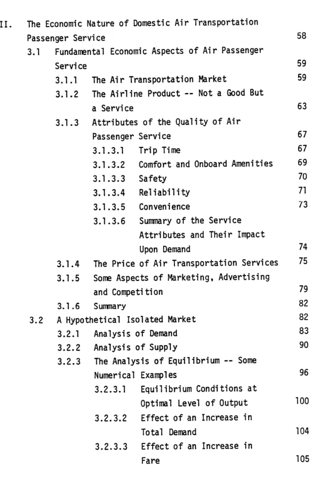
III. The Economic Nature of Domestic Air Transportation Passenger Service
3.1 Fundamental Economic Aspects of Air Passenger Service
Page
58
3.1.1 The Air Transportation Market
3.1.2 The Airline Product -- Not a Good But a Service
3.1.3 Attributes of the Quality of Air Passenger Service
3.1.3.1 Trip Time
3.1.3.2 Comfort and Onboard Amenities 3.1.3.3 Safety
3.1.3.4 Reliability 3.1.3.5 Convenience
3.1.3.6 Summary of the Service Attributes and Their Impact Upon Demand
3.1.4 The Price of Air Transportation Services 3.1.5 Some Aspects of Marketing, Advertising
and Competition 3.1.6 Summary
A Hypothetical Isolated Market 3.2.1 Analysis of Demand 3.2.2 Analysis of Supply
3.2.3 The Analysis of Equilibrium -- Some Numerical Examples
3.2.3.1 Equilibrium Conditions at Optimal Level of Output 3.2.3.2 Effect of an Increase in Total Demand 3.2.3.3 Effect of an Increase in Fare 3.2 59 59 63 67 67 69 70 71 73 74 75 79 82 82 83 90 96 100 104 105
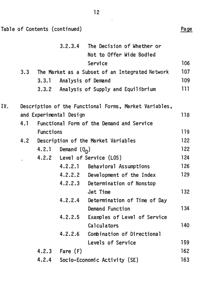
Table of Contents (continued) Page
3.2.3.4 The Decision of Whether or Not to Offer Wide Bodied
Service 106
3.3 The Market as a Subset of an Integrated Network 107
3.3.1 Analysis of Demand 109
3.3.2 Analysis of Supply and Equilibrium 111
IV. Description of the Functional Forms, Market Variables,
and Experimental Design 118
4.1 Functional Form of the Demand and Service
Functions 119
4.2 Description of the Market Variables 122
4.2.1 Demand (QD) 122
4.2.2 Level of Service (LOS) 124 4.2.2.1 Behavioral Assumptions 126 4.2.2.2 Development of the Index 129 4.2.2.3 Determination of Nonstop
Jet Time 132
4.2.2.4 Determination of Time of Day
Demand Function 134 4.2.2.5 Examples of Level of Service
Calculators 140
4.2.2.6 Combination of Directional
Levels of Service 159
4.2.3 Fare (F) 162
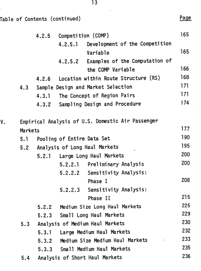
Table of Contents (continued)
4.2.5 Competition (COMP)
4.2.5.1 Development of the Competition Variable
4.2.5.2 Examples of the Computation of the COMP Variable
4.2.6 Location within Route Structure (RS) 4.3 Sample Design and Market Selection
4.3.1 The Concept of Region Pairs 4.3.2 Sampling Design and Procedure
V. Empirical Analysis of U.S. Domestic Air Passenger Markets
5.1 Pooling of Entire Data Set 5.2 Analysis of Long Haul Markets
5.2.1 Large Long Haul Markets
5.2.2.1 Preliminary Analysis 5.2.2.2 Sensitivity Analysis:
Phase I
5.2.2.3 Sensitivity Analysis: Phase II
5.2.2 Medium Size Long Haul Markets 5.2.3 Small Long Haul Markets
5.3 Analysis of Medium Haul Markets 5.3.1 Large Medium Haul Markets
5.3.2 Medium Size Medium Haul Markets 5.3.3 Small Medium Haul Markets
5.4 Analysis of Short Haul Markets
Page 165 165 166 168 171 171 174 177 190 195 200 200 208 215 225 229 230 232 233 235 236
Table of Contents (continued)
VI. Applications of the Models
6.1 Derivation of Demand Vs. Frequency Relationships 6.2 The Impact Upon Demand of New Technologically
Advanced Aircraft
6.2.1 The Introduction of a Supersonic Transport on Long Haul Domestic Routes
6.2.2 The Introduction of a Fuel Efficient Subsonic Aircraft on Medium Haul Routes
6.3 Aggregate Forecasting
VII. Conclusions and Recommendations for Future Research
Appendix A.
Appendix B. Appendix C.
List of Region Pairs by Demographic Stratifications
The Hat Matrix in Linear Models
Multicollinearity and Related Topics C.1 Singular Value Decomposition C.2 Principal Components Bibliography Biographical Sketch Page 240 241 247 249 250 253 255 260 268 278 281 285 291 296
15
I. Introduction
The process of forecasting the demand for air transportation services has in recent years become an extremely complex operation. Since the late sixties, when the United States domestic air carriers suffered through a grave financial crisis, industry analysts have recognized the sensitivity of the fiscal strength of the airlines and aircraft manufacturers to their planning process, which is based upon travel demand forecasts. Furthermore, the analysts have realized that traditional forecasting methods such as trend extrapolation are inadequate due to the impact upon travel demand of recent changes within the economic and operating environment such as high
inflation rates, escalating fuel and labor costs, and uncertainties with regard to future technology and regulatory conditions.
The past performance record of air traffic demand forecasters has been unimpressive. Forecasting models based upon methodologies with a low level
of sophistication have not, as mentioned above, captured the impacts of important demand and/or supply determinants. Models based upon more
sophisticated methodologies, such as advanced econometric techniques, have generally been limited by either insufficient understanding of the total air transportation system or by lack of relevant data.
In his introductory remarks in a talk entitled, "Air Transportation --Directions for Future Research" presented at a workshop on air
transportation demand and systems analysis in June 1975, George Avram of Pratt and Whitney Aircraft cited the findings of a survey recently conducted by Brushkin Associates. The findings indicated that people gave a very
favorable rating to the forecasting accuracy of sportswriters, sports announcers, and weathermen. At the opposite end of the spectrum, those forecasters who received the least favorable ratings included stock brokers, astrologers, and economists. Mr. Avram's reaction to this was that "since economics is the cornerstone of our understanding of the present and the future...we (sic) got a lot of work to do!"'
Although this dubious honor was directed at economists in general, Mr. Avram was singling out forecasters of the levels of future activity in the air transportation industry. His remarks are indicative of a general dissatisfaction of airline companies, aircraft manufacturers, airport authorities, and regulatory agencies with the accuracy of the forecasters' predictions.
1.1 The Role of Demand Forecasting in the Air Transportation Industry Two fundamental questions arise when considering the role of demand forecasting in the air transportation industry:
(1) Is it necessary to forecast air traffic demand, and
(2) What is the importance and role of the forecasting process? This section will address these questions from the perspective of three different components of the commercial aviation system: the airlines, the airport authorities, and the equipment manufacturers.
1 "Proceedings of the Workshop: Air Transportation Demand and Systems Analysis" (Cambridge: M.I.T. Flight Transportation Laboratory Report R75-8, August, 1975), pp. 452-456.
1.1.1 Demand Forecasting and the Airlines
The basic function of demand forecasts to the management of the airline companies is to provide input to the planning processes. The adverse effects of planning decisions made by airline companies based on
inaccurate forecasts can be clearly illustrated by examining the plight of the industry during the late 1960's and the early part of the 1970's.
Throughout the early and middle sixties, aggregate domestic traffic had been growing exponentially, at a fairly constant rate of between ten and fifteen percent per year. As the sixties progressed, it became necessary for the airlines to continually increase frequency of service to satisfy the growing demand and to maintain reasonable load factors. This expansion of service began to cause serious delays at major airports, resulting in considerable inconvenience to the passengers and expense to the carriers.
Assuming that the levels of passenger demand would continue to grow at the 1960's rate, the airlines decided to introduce wide-body aircraft with two to three times the seating capacity of the narrow-body aircraft in use at that time. The carriers could then greatly reduce frequency while maintaining reasonable load factors, thereby satisfying consumer demand, relieving congestion, and reducing per-passenger cost.2
These planning decisions would have provided fruitful results, had the demand forecasts been accurate. What in fact did occur was a sharp
decline in passenger growth in the late sixties and beyond, and the airlines were producing a lower level of service (to be formally defined
in Chapter IV), load factors declined, and costs soared. This alarming situation caused the carriers to recognize the importance of accurate forecasting and the need for improved forecasting methodologies. This condition is aptly characterized by Harry G. Lehr, Director of Regulatory Affairs of United Airlines:
"We know from hard experience the difficulty airlines- have had with [forecasting] and considerable talent has been applied to this problem. Yet, I would characterize the development of our forecasting ability as having reached a level that can only be referred to as Organized Soothsaying. The current economic conditions of the industry and the perishability of our product.. .dictate a need for a forecasting methodology that is substantially closer to the level of development of our other planning tools." 3
1.1.2 Demand Forecasting and the Airport Authorities
The need for improved forecasting of air transportation is equally as great for airport authorities as for the carriers. In recent years
sophisticated models, based upon operations research and simulation techniques, have been developed to measure airport runway capacity and hence the airport's ability to control delays and delay costs4 and to measure passenger flow'through terminals.5 However, the ability of
"Proceedings of the Workshop", p. 160.
For example, see Gerd Hengsbach and Amedeo R. Odoni, "Time Dependent Estimates of Delays and Delay Costs at Major Airports (Cambridge:M.I.T. Flight Transportation Laboratory Report R75-4, January, 1975).
For example, see Terry P. Blumer, Robert W. Simpson, and John Wiley, "A Computer Simulation of Tampa International Airport's Landside Terminal Shuttles" (Cambridge:M.I.T. FTL Report R-76-5, April, 1976).
these models to evaluate future airport design is only as good as the input data, such as expected number of aircraft movements and passenger
enplanements, provided by forecasting models.
George P. Howard, Chief of Aviation Economics of the Port Authority of New York and New Jersey, emphasizes this need for good input data:
"If one considers that Port Authority investment in the three metropolitan airports to date is some one billion dollars and that airlinesand other tenants have invested very significant amounts of their own money in these facilities, there is no need to question the desirability, indeed the necessity, of market forecasts which project, as accurately as possible, future trends in the air transportation market in the New York/ New Jersey area." 6
1.1.3 Demand Forecasting and the Equipment Manufacturers
Forecasts of future air traffic is also essential to the manufacturers of aircraft and aircraft engines. The need is particular great in this case not only for forecasts of aggregate traffic (in system revenue
passenger miles, for instance), but for forecasts by density and length of haul of the various markets, since design parameters of an individual
aircraft type (and its engines) are based upon its desired range and seating capacity. John D. Karraker of General Electric elaborates: 6 George P. Howard and Johannes G. Augustinus, "Market Research and Forecasting for the Airport Market", in Airport Economic Planning, ed, George P. Howard(Cambridge:M.I.T. Press, 1974), p. 109.
"The nature of our product, the jet engine, demands long range planning. It costs in the neighborhood of half a billion dollars and takes from 5 to 10 years to develop a new jet engine from the concept stage to commercial service. As you can well appreciate, an error in determining the potential market for a given engine can have very grave consequences in our business. Obviously, the minimizing or avoidance of such costly errors is a necessity. For this reason, forecasting is recognized in General Electric as one of the major elements of.our business." 7
1.2 The Need for Policy Sensitive Forecasting Models
The above arguments all indicate a strong need for models that
forecast levels of traffic, whether it be over the entire system or subsets of the system, as in the case of the airlines; or into, out of, and through, particular cities, as in the case of the airport authorities; or over sets of market types, as in the case of the manufacturers. Some of the more recently developed models are quite capable of predicting reasonable
estimates of traffic.8 However, as will be argued in Chapter II, none of the current models is sufficiently policy-sensitive to determine within a given market the impact of such economic alterations as route awards, fare changes, modifications in quality of service, and acquisition of new
equipment. So, while traffic can be forecasted based upon exogenous factors assuming that the variables under the control of the carriers and regulators remain basically stable, no conditions have been introduced into existing models to demonstrate how the carriers and regulators can them-selves influence traffic levels within the individual markets.
"Proceedings of the Workshop", p. 445.
8 For example, see "Aviation Forecasts, Fiscal Years 1976-1987" by the Federal Aviation Administration, summarized in Chapter II.
An example of where a policy-sensitive market demand model would be useful is in conjunction with fleet assignment optimization models.
Several such models have been developed by equipment manufacturers and by academic institutions. One example is FA-4, a model developed in the Flight Transportation Laboratory at M.I.T.9 FA-4 is a very sophisticated linear programming model which allocates a mixed fleet of aircraft over a route network so as to maximize the difference between total revenue and the sum of direct and indirect operating costs. The optimization is constrained by a number of economic factors including, among others, prescribed load factor conditions, fleet availability, minimum number of departures in the various markets, and maximum number of departures from
the various stations.
While FA-4 is very realistic in its modeling of the attributes of an airline's fleet allocation problem, it is limited by the fact that it requires a set of rather ad hoc piecewise linear demand vs. frequency
curves as input. If a demand model existed which adequately estimated the response in passenger traffic as a function of level of service ( as well as other factors such as fare and regional demographics), more confidence could be placed in the output of this otherwise-acceptable fleet
assignment model.
9 Swan, William, "The Complete FA-4 Memo" (Cambridge: M.I.T. FTL Technical Memorandum 72-10, August, 1972).
1.3 Purpose and Outline of This Thesis
The purpose of this thesis is to develop a set of demand models whose parameters are a function of length of haul and demographic size of the markets. These models will be sufficiently policy sensitive so as to
forecast the impacts upon market demand of changes in such factors as quality of service, competition, fares, equipment, and regional demography.
There are basically four reasons why these models will constitute an improvement over existing models. They are as follows:
(1) The models will be multi-equation in structure. This advanced specification was chosen to eliminate the coefficient bias present in single-equation models, caused by simultaneity between supply and demand variables.
(2) The variables will be more complete by definition. Many of the proxies used to calibrate existing models have been too simplistic in definition and do not fully measure the levels of important demand and
service-related attributes.
(3) The experimental design will be more complete. This will assure not only a larger sample size, but also a more representative subset of U.S. domestic markets with respect to length of haul and to socio-economic factors.
(4) Advanced techniques will be employed to assure statistical robustness and high precision of coefficient estimates.
introductory chapter will be elaborated upon in Chapter II, which reviews some published studies in air transportation demand analysis. Preceding this review will be an overview of general transportation demand theory. The discussion in Chapter II will focus on how the air transportation models have been developed as various aggregations of the general theory and how the models which will be developed later in this thesis fit into the aggregation process.
Based upon the general economic theory of transportation demand, and upon the issues raised in the development of the models surveyed in Chapter II, an economic theory of domestic air transportation service will be presented in Chapter III. This discussion is essential for providing a detailed explanation of errors of omission, for the models surveyed in Chapter II, of important supply and demand related attributes. Further-more, the contents of Chapter III provide the necessary coverage of issues that will, and will not, be important in the development of the resulting models in this research. The end product of Chapter III is a general specification of the models to be calibrated.
Chapter IV takes the general model developed in Chapter III and more precisely identifies the specification. The complete definitions of the variables are presented in Chapter IV, and numerical examples of the computation of the more complex proxies are provided. The sampling
procedure is also detailed in Chapter IV.
Chapter V contains the results of the empirical calibration of the models specified in Chapter IV. Special attention is given to the
24
product of Chapter V is a structural demand analysis equation for each stratification of markets, separate demand equations are produced for forecasting and analytical (policy sensitivity) purposes.
Chapter VI applies the models calibrated in Chapter V to measure the impact upon demand within given markets due to changes in future
technologies and fare structures. Chapter VI also outlines how the models may be applied for aqcregate demand forecastin. Chapter VII contains the
II. Overview of Transportation Demand Theory and Domestic Air Transportation Economic Models
The introductory chapter described the motivation for economic models that forecast the imDact upon air passenger demand within domestic markets of policy changes within the industry. Furthermore, it was mentioned
therein that the performance of existing models, particularly in the sense of policy analysis, has generally been quite disappointing. In this chapter, an overview of the economic theory of travel demand, particularly with respect to the air mode, will be presented. The development of five existing models based upon this theory will be studied, and their strengths and weaknesses with respect to their reliability for forecasting and
analysis will be identified.
The main variant in the structure of transportation demand models is their level of aggregation. A totally disaggregate model would specify
the consumption optimization problem for each consumer (or group of equivalent consumers) in the population. The decision of how many air trips from each consumer's origin to a specific destination in a given time period would be a function of not only the characteristics and prices of these trips, but also of the characteristics and prices of all other transportation services available to this consumer. These other services
include trips to all other destinations and to the same destination by alternative modes. Summing over all consumers would yield estimates of total demand in all markets and by all modes,
total disaggregation intractable, researchers are forced to combine some or all factors. Some models of air transportation demand do not consider the effect of competing modes and/or destinations. Other models do not recognize distinct groups of consumers, such as by income levels, and instead focus on aggregate regional or national economic variables. Another level of aggregation is by markets whereby a model would not measure demand from point to point, but over a large mass of origin-destination pairs such as the Northeast Corridor. Total aqgregation combines all of these factors and qenerally forecasts a sinqle variable such as revenue passenger miles for the entire domestic system.
2.1 Total Disaggregation
Lancaster, in his recent theory of consumer demand,1 asserts that individual consumers select goods and services based upon the
"characteristics" of these products, where the characteristics are "those objective properties of things that are relevant to choice by people."2 For example, the scheduled flight time of an aircraft departure is certainly a characteristic of this product, whereas the color of the aircraft is a property that is not likely to be a characteristic.
The primary difference between Lancaster's demand theory and
traditional consumer demand theory is that Lancaster's theory states that
1 Kelvin Lancaster, Consumer Demand: A New Approach (New York: Columbia University Press, 1971).
a consumer will maximize a utility function which is dependent upon characteristics, rather than upon the goods themselves. Assuming that the characteristics of various products are indeed objective and
quantifiable and that their levels are linearly related to the levels of the product, the following relationship holds:
z = Bx (2.1)
where
z = an m by 1 vector of characteristics x = an n by 1 vector of products
and B = an m by n matrix of coefficients relating the products to the characteristics called the "consumption technology matrix". An important point is that the consumption technology matrix, B, is invariant among consumers. A given product is viewed by each consumer as bearing the same levels of characteristics; however, consumers will react differently to these characteristics. Two reasonable people would
assumedly not argue over size, ride quality, handling, performance, etc., of different types of automobiles. However, they may purchase different autos because of their relative desires and preferences for these various
characteristics.
Given that each consumer is constrained in consumption by his budget, the following mathematical program is formulated:
Max U = U(z)
Tx >k
where
p = an n by 1 vector of prices of products and k = the consumer's income.
Since the consumption technology matrix, B, and the price vector, p, are assumed identical for all consumers, and the utility function, U(z), and the budget, k, will vary among consumers, levels of demand for various products can change due to two distinct classes of effects. The
"efficiency effect" is the result of a change in product technology, b (the column of B referring to project
j),
or price, pj, and is perceived by all consumers. The "demand effect" is the result of changes in an individual's needs and preferences for various characteristics, manifested in U(z), or changes in an individual's income, k. The demand effect is obviously an individual consumer phenomenon.Quandt points out that "...travel is viewed as the result of individuals' rational decision making in an economic context."3 Since this point is very difficult to argue, it appears as though the analysis of travel demand by the consideration of the maximization of individuals' utility functions is a sensible approach. However, if one were to exploit the full power of the above theory, the researcher is forced to develop a set of demand models that are stratified by many factors. The parameters of the model would vary by income group, as it has been shown that the
3
Richard E. Quandt, The Demand for Travel: Theory and Measurement (Lexington, Mass.: Heath Lexington Books, 1970), p. 1.
amount of travel and the modal split are related to personal income.4 Furthermore, the utility functions will vary by demographic groups. For example, an individual's occupation may affect his utility for travel related characteristics, distinct from the income effect.5
Lancaster develops the notion of "natural" or "intrinsic" groups of products, based upon the structure of the consumption technology matrix.6
An intrinsic group is a subset of the available products that relate to a subset of characteristics, such that no products outside of this subset possess positive levels of any of the related characteristics.
Further-more, no product in the subset possesses positive levels of any
characteristics not in the related characteristic subset. If indeed an intrinsic group does exist, the consumption technology matrix can be written as follows:
B
= [(2.3)
where B1 is the subtechnology of the intrinsic group and B2 is the subtechnology of the remainder of the products in the market.
All of the transportation demand models that were surveyed prior to this research assume that transportation services comprise an intrinsic
4 Philip K. Verleger, Jr., "A Point-to-Point Model of the Demand for Air Transportation" (Ph.D. dissertation, M.IT., 1971), p. 79.
Quandt, op. cit., p. 12.
group. Since efficienty substitution effects are the attainment of a new characteristics vector due to a change in the mix of products purchased caused by a shift in the consumption technology matrix or price vector, this assumption implies that efficiency substitutions cannot occur between transportation services and other products. Consequently, prices and characteristics of non-transportation products are generally not included
in transportation demand models.
The individual's optimization problem for transportation services can now be formulated as a subprogram of (2.2) as follows:
Max Ut = Ut(zt subject to zt = Bt xt (2.4) T <~ p tx t- kt xt 0 where
Ut= the utility function of characteristics related to
transportation service characteristics
z = the set of transportation service characteristics Bt = the transportation technology matrix
xt the set of available transportation services Pt= the price vector of transportation services
kt = the amount of the individual's income that can be afforded for transportation services
A totally disaggregated demand model must then consider the following elements:
(1) sensitivity to different consumer groups, particularly with respect to income levels;
(2) sensitivity to price and characteristics of competing modes; (3) sensitivity to price and characteristics of competing
destinations.
Since the inclusion of all of the above elements is obviously intractable, researchers are forced to aggregate some or all of them. The remainder of this chapter will provide a survey of models indicating how these aggregations have been performed.
2.2 Aggregation by Destinations
Reuben Gronau, in his Ph.D. dissertation at Columbia University which was later published as a book, developed a model sensitive to income groups and modal split, but did not explicitly account for consumer choice of alternate destinations. Because of data restrictions, this model was calibrated for trips in and out of New York City over the 38 most heavily traveled New York markets. Since this is a cluster sample, there would
likely be considerable bias if one were to attempt to apply these results to the entire U.S. domestic system.
Reuben Gronau, The Value of Time in Passenger Transportation: The Demand for Air Travel, National Bureau of Economic Research Occasional Paper 109 (New York: Columbia University Press, 19701.
Gronau altered Lancaster's theoretical 'model (2.4) by defininq the utility function over an "activity" space, rather than over characteristic space. The activities, z., are packaged combinations of market products, xi, and time, T.1.
z = fi(xi, Ti) (2.5)
One type of activity, he states as an example, is a "visit" which is a combi-nation of transportation, hotel and restaurant services, travel time, and time at the destination.8
A second modification to Lancaster's theory is that Gronau considers time as a constraint analogous to the income constraint in (2.4). One of the objectives of this research was to evaluate a monetary value of time for various income groups, and, as will be shown, the inclusion of the set of time constraints facilitates this in theory.
The consumer's optimization problem for travel activities is then as
follows: Max U = U(z., zn2 ... , zn) n subject to E P. x. = Y (2.6) i=l1 n Z T. = T0 i=1
where pi = price of market product x i
Y = the consumer's monetary travel budget
T, = time investment for product x.
T 0 the consumer's travel time limit9
The Lagrangian of (2.6) can be written as follows:
L = U(z1, Z2, ... , Zn) + X(Y - EP x ) + i(T0 - ET ) (2.7)
The first order conditions for optimization of (2.7) are:
3x. 3T.
a - XP 31y - (2.8)
1
3z zi 1 a 1
Gronau then defines K = y/X as the shadow price of time.
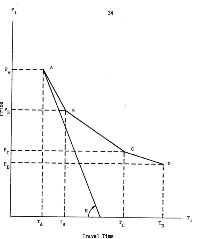
Assuming that there are four modes of travel, A, B, C, and D, between two cities, that the only two attributes of modal choice for a consumer deciding to travel between the cities are price and travel time, and that none of these modes is dominated by another in terms of these attributes, the consumer will choose the appropriate mode based upon his value of K. This is depicted in Figure 2.1, where points A, B, C, and D are the location of the modal attributes in price/travel time space. The line ABCD is the convex envelope of these four points. A generic consumer will select that mode represented by the extreme point of the convex envelope
9 Since, as previously noted, transportation services are generally considered as constituting an "intrinsic group", all products,
characteristics, and activities will hereafter be assumed as being related only to transportation services. For simplicity the "t" subscripts
34 pA _- A I B p C C P D D A T. TA TB T C T D Travel Time
Figure 2.1 Gronau's Moda Choice Representation for a Given City Pair
35
which is tangential to a line with- slope -K. In the example shown in
Figure 2.1, this would be mode A.
More formally, if one assumes that the traveling process has no utility in itself, and hence the various modes may be considered as
different combinations of the price and time attributes, then the "marginal rate of substitution", K* ., between modes i and j can be defined as the absolute value of the slope of the line segment between i and j.
P. - P.
K*.. = T (2.9)
13T - T.
Mode i will be preferred to mode j if K* > K.
Since prices and travel times between cities for any given mode are generally linear functions of intercity distance, Gronau concludes that
the general modal choice decision is a function of K and of distance. For example, based upon numerical estimates of trip times and fares, he concludes that for a 150 mile trip, "a passenger prefers to use air rather than rail transportation....only if his price of time exceeds $11.80 per hour, he prefers air to bus if his price of time exceeds $7.10 per hour, and he prefers rail to bus if his price of time exceeds $5.30 per hour. Bus transportation is, therefore, used for 150 mile trips only for individuals whose price of time is less than $5.30 per hour."1
The specifications of Gronau's demand model are as follows:
x = r 1jU Y 2j eu (.2.10)
where
x = number of trips to destination
j
per family of income group i Tr.. = generalized trip cost = P. + K.T.Y = average income for income group i ui = disturbance term
Bj2 ,lj, and a2j are regression coefficients.
Assuming that the price of time is proportional to hourly wages, K = kW., and taking logs (2.10) becomes:
log x = log B. + 81. log (P. + kW1Tj) + a23 log i + u.
(2.11) -Finally, the assumption is made that alj and a2j are independent of
the destinations and adding an "attractiveness" factor for each destination
j,
G., the model (2.11) becomeslog xg = ao + Ig log(Pg + kW) T + S2log Yi + elog G
+ uij (2.12)
The income and traffic data used to calibrate equation (2.12) was extracted from onboard passenger surveys conducted by the New York Port Authority. These surveys provide demographic and travel frequency data on a sample of local New York passengers (connecting passengers were excluded) conducted from April 1963 through May 1964. Travel time was taken to be the fastest scheduled flight on each route plus average
was standard coach fare plus limousine fare from downtown to the airport. The level of attractiveness variable, G, is a function of the
population of the destination city's SMSA and the number of phone calls made between the two cities. The latter factor presumably was selected as
a result of previous research by Brown and Watkins.12 While the number of phone calls may be an adequate attractiveness variable for the purpose of Gronau's research, to measure monetary value of time, it is doubtful that
this variable would be useful in a forecasting model. The number of phone calls are probably no easier to forecast than the response variable, air passenger trips.
The estimation procedure that Gronau used was a nonlinear search technique in which the variable k was varied from zero to two -- by increments of 0.25. While the coefficients of all the variables had the correct sign and were highly significant, and the R2 values were
reasonable (all generally between 0.8 and 0.9), the effect upon the fit of varying k was nearly negligible, usually only changing the third decimal place of R2.
A major flaw in Gronau's specification is the definition of travel time (fastest scheduled flight plus driving time from center city to airport). One limiting assumption is that a person desiring to fly will be able to board the "fastest" flight at his convenience; this completely
12 Samuel L. Brown and Wayne S. Watkins, "The Demand for Air Travel: A Regression Study of Time Series and Cross Sectional Data in the US. Domestic Market, " in Airport Economic Planning, ed. George P. Howard (Cambridge: M.I.T. Press, 1974), p. 99.
ignores the existence of schedule delays. Secondly, the inclusion of driving time from the center city to the airport is appropriate only if all travelers originate in the center city. Finally, the travel time is likely to be a function of route density. This creates a simultaneity problem which requires a multiple equation system to assure unbiasedness in the estimates.
2.3 Aggregation by Incomes
Terry Blumer created a city pair air transportation demand model for short haul (less than 400 miles) markets in his master's thesis from
13
M.I.T. His "base model", a common gravity model which aggregates by income groups and does not consider the effect of competing modes and/or destinations, is shown below:
M.M. bI b2
T.. j J I.. (2.13)
b0 Dii ija where
T.. = air traffic between cities i and j 13
Mi = effective buying income of city i
Iija = disutility of air travel, "air impedance", between i and j D.. = distance from city i to city
j
The term "gravity model" stems from the comparability between quantity of travel between two cities and gravitational attraction between two
13
1 Terry P. Blumer, "A Short Haul Passenger Demand Model for Air Transportation" (S.M. Thesis, M.I.T., 1976).
physical bodies. Both are positively related to the mass of units and negatively related to the distance between them.
A major improvement of this model over conventional gravity models is the explicit inclusion of a level of service variable, Iija. This variable is a prototype of LOS, the level of service variable developed
by Eriksen for the research of this dissertation, and explained in detail in Section 4.2. The impedance variable is a generalized trip time which considers not only the number of daily available flights, but also time of day of departure, number of intermediate stops and/or connections, and speed of aircraft.
Blumer then expanded his base model by developing a "mode sensitive" model consistent with the concept developed in Section 2.1 that air travel will be sensitive to the characteristics of competing modes. He defines
Ti,
the "total transportation impedance", in a given city pair, as follows:-2 2 + 2 j + 21 (2.14)
2
i j 1 i j a ij u ij r
where I and I.. are impedances for auto and rail, respectively, The mode sensitive model is then defined as:
T.. = b i ) . . f . (2,15)
13 0 D ) 13 fij
The f variable was described several different ways each of which was some function of the relative impedances of air and surface modes.
The next step was the development of a "destination sensitive" model based upon the assertion that "...[the presence of alternate destinations in close proximity to market i to
j]
has the effect of decreasing the number of trips made to j and may possibly increase the total number of trips generated by city i due to (the alternate destination's] own unique attractions."14 This again is consistent with the theory developed in Section 2.1, which implies that air travel will be sensitive tocharacteristics of trips to competing destinations.
The destination sensitive model is defined as follows:
T. = b0H (M, M , S , S ) bI b 2 F 3 (2.16)
where
H. = air travelers generated by the cities i and j (to all destinations)
S = total attraction of alternate destinations for travelers from city i
and F = fraction of total travelers generated by regions i and j that move from i to j or from j to i.
Finally, Blumer combined the models shown in (2.13), (2.15), and (2.16) to obtain a set of six "mode and destination sensitive" models, 14 Ibid., P. 47.
After calibrating these using various data sets he concluded, on the basis of highest R2, that the best model was as follows:
61 62 b1 b2 b3 b4
T. = b (M. i + M. 2) I D. 0. F.. (2.17)
13 0i 1 j1a 13 13
where 61 and 62 are constants determined by nonlinear search.
The data used in the calibration of the "best" model, (2.17), was a pooling of two years of cross sectional data. All coefficients were highly significant and had correct signs. The R2 value was 0.90, and an extensive set of statistical tests indicated no violation of the normal least squares regression assumptions (consistent pooling, homoscedasticity, normality of residuals, etc.).
Blumer addresses the fact that aggregating over income distribution may be a somewhat limiting assumption.
"It might be said that neither population nor income truly measures the ability of a city to generate travelers. Population is poor because a large city would still not produce many travelers if all residents were poor. Income also has shortcomings in that, if used alone, it assumes every dollar has the same propensity to generate a trip
--a [person] who is twice as rich will take twice as many flights. Surveys taken indicate the flight generation
is not linear with income, but increases at an increasing rate (for the income levels sampled). 15
He suggests, as a future research topic, the development of a more general
mass variable which assumes that the function relating household income levels to number of trips varies by mode:
R K
M. = Z N. (r) Z H. (r) (2.18)
r=1 m=l where
r = index of income levels
R - number of predefined income levels
N (r) number of households in city i in income level r m = index of modes
K number of modes
H. (r) average number of trips by mode m per household of income level r
An obvious shortcoming in what otherwise is an exceptionally good model is the simultaneity of the response variable, T , and the impedance term, Iija' Blumer realizes and addresses this weakness again within the rubric of future research.
"Another area to explore is a second [equation in the ] model representing service. Obviously the number of flights depends upon the demand and the demand depends upon the number of flights. This two way causality suggests building a second [equation] representing air service to be solved simultaneously with the first [equation]. This would also eliminate the requirement to forecast air service, since it would become an endogenous variable." 16
2.4 Aggregation by Modes and Destinations
in his doctoral dissertation at M.I.T., Philip Verleger constructed a "point-to-point" model of air transportation demand.17 The purpose of this research was not to construct a forecasting model, but rather a model to test if demand relations vary across markets. This, in turn, would thereby test the validity of cross-sectional and aggregate models. The models proposed and tested by Verleger were similar in the respect that, while they were city pair oriented, they did not consider the effects upon air traffic demand due to the existence of competing modes and destinations,
The structure of the model that was calibrated over all routes in his sample follows:
T = P.. X(M.M.)y (SEA 1)"' (SEA 2)a2 (SEA 3)t E (2,19)
ij1 1 j
where
T.. = air travel between cities i and j P.. air fare between cities i and
j
13
Mi = mass of city i
and SEA 1, SEA 2, SEA 3 = seasonal dummy variables.
The price variable? Pi, is an index formed by weighting the major airline fares; first class, coach, family, And discounts, For routes in which the fare usage data were not available, they were estimated by
taking those values for "similar" routes. "Thus the weights for Cleveland
17 Philip K, Verleger, "A Point-to-Point Model of the Demand for Air
to New York were used for Cincinnati to New York."18
A major contribution of this research was Verleger's handling of the income distribution effects. He argues that population alone as a mass variable (a common occurrence in gravity models) assumes that either
income distributions are constant among cities or that the proclivity of people to travel is independent of their income. Since the former point
is known to be false and the latter has been refuted by many surveys, Verleger chose to disaggregate the traveling populations by income.
The definition of his mass variable is as follows:
N Z
YX
M = Z xA e (2.20)
where
2. e index of income groups in city i N = number of predetermined income groups x~ weighting of group
S = regression coefficient
Y X average income of group
The estimation of the parameters of the model (2.19) required a nonlinear regression technique, and a special algorithm was written. An iterative procedure was devised by searching for the value of a (a. and a, were assumed equal in a given city pair ij) that minimized the variance.
In nearly all markets (108 of 115) a positive estimate for resulted, and in most of these markets it was statistically significant (79 of the 18 Ibid., p. 112.
108 were significant at the 95% level), In addition to this, the overall income coefficient y was positive in all but one market (Boston-New York) and significant in 105 markets,
The general conclusion atrived at by the author is that air travel
is
"very income elastic"19 and only weakly responsive to price changes, as the price elasticity showed no regular pattern and was negative andsignificant in only 20% of the markets. The mean price elasticity was -0.12 with a variance of 0.45. The author concluded that it is inadvisable to interpret aggregate measures of price elasticity with any confidence.20
The author proceeds to analyze the fare effect by density. The results show that in the more heavily travelled markets, the fare
elasticities have a tendency to be more uniformly significant, While in the low density markets few are significant. The author suggests that the variance of the price coefficient decreases as traffic increases, and that in aggregate analyses a weighted least squares estimation procedure should be used to eliminate this bias. However, it is possible that the implied weak impact of fares is due to the omission of a level of service variable. In dense markets the service will be greater than in the sparse markets, and inclusion of a level of service variable may therefore strengthen the significance of the price variable by reducing the variance of its
coefficient. In other words, the level of service variable would provide
19 Ibid., p, 186,
an economically justifiable set of weights and then ordinary or preferably two-stage least squares could be used to estimate the coefficients.
2.5 Aggregation by Incomes, Destinations, and Modes
A two-equation city pair economic model of air transportation service was developed by Pat Marfisi in his Ph.D. dissertation at Brown
Univer-sity.21 The purpose of this research was to model the capacity decision process of an airline firm within a given market when faced with
uncertainty of future demand. This study was an innovative contribution to the research in air transportation economics, in that an attempt was made to build a comprehensive model of the supply side that would be
compatible with the demand so that both could be solved simultaneously. Aside from the statistical problems inherent with the simultaneity situation with single equation models, Marfisi states the following:
"Economists argue on the basis of theory that an increase in fare levels will increase market equilibrium capacity. It is argued here that this is not an unambiguous
implication of economic theory but rather an empirical question regarding the relative magnitude of certain demand elasticities; a judgement which has never been tested by a statistically consistent procedure. Concurrent with the discussion suggesting a theoretical link between fare levels and capacity, other economists are estimating demand functions for scheduled air transportation based on econometric models that implicity assume the absence of any linkage between the demand and supply side of the
21 E, Pat Marfisi, "Theory and Evidence on the Behavior of Airline Firms Facing Uncertain Demand" (Ph.D. dissertation, Brown University, 1976).
market (i.e., demand does not constrain or alter supply behavior and vice versa." 22
Marfisi's discussion is segmented into two somewhat disjoint sections. The first section is a quite comprehensive economic theory of the supply
side of the industry. The- second half is an empirical study of his two-equation model. The major conclusion of the theory is that the use of a
single-equation model to estimate price elasticity implicitly assumes that dP= 3P , where
Q is demand and P is price.
Marfisi's theory arrives at the relationship where, if demand is differentiated with respect to price, the result is ;= + . d, where C is capacity. Since it is unclear as to what is the sign of the derivative of capacity with respect to price, then r may well be positive. The result is that positive price coefficients in reduced form equations are indeed consistent with economic theory and explain the somewhat embarrassing results of some economists(e.g., Verleger 23), who misspecify
a
reduced form as a structural form system and obtain positive price elasticity estimates.The structural form of the model used for Marfisi's empirical study is as follows: B1 y'l Y2 3h
Q
=C P Y'I p C2,20) B2 4 5 6 7 C =Q P W E N 22 Ibid., p, 2-17. 23 Verleger, op cit., p, 188,where
Q = origin to destination passenger demand C = flight frequency
P fare
Y per capita income p population
W a average cost per flight N number of competing firms
= measure of demand dispersion
The capacity variable is more formally defined as the number of nonstop and one-stop scheduled flights. While the inclusion of a level of
service variable is praiseworthy, this definition is restricting. Such important aspects as the relative number of nonstops to one-stops, whether the one-stops are direct or connecting, the speed of the aircraft, and the time of day scheduling, are not reflected in this measure.
The competition variable, number of competing firms (airlines), is also a very important addition in this model, but its definition is also somewhat crude. The variable was assumed to be the number of airlines in a market that provide at least five percent of the capacity. By this specification, a highly competitive market such as Chicago/Los Angeles, which is served by four strong carriers, would be considered the equivalent
in competitive structure of a market in which one major carrier provides eighty percent of the capacity while three other minor competitors evenly provide the remainder.
from this study. Marfisi stratified the markets by purpose of trip and length of haul and conducted a series of Chow tests to investigate the appropriateness of aggregating markets across these strata. The
conclusions indicate that the underlying structural relationships between market variables are substantially different. This is to be expected, as it is generally believed that business travel is considerably less price elastic than non-business travel. Furthermore, the structural
relationship for markets of less than 200 miles are significantly different than that of markets greater than 200 miles. This effect is due
presumably to the presence of competing modes in the short haul markets. The analysis showed, however, that no significant differences in the
structural relationships exist between medium and long haul markets.
2.6 Total Systemwide Aggregation
The most common approach to econometric modeling of air transportation demand is the total systemwide aggregate model. These macroeconomic
models predict a single figure for the industry, revenue passenger miles (RPM). While these models are generally very accurate in terms of
forecasting, they are restricting in two respects. The first limitation is that they are inappropriate for measuring the impacts of policy
decisions (e.g., changes in fare or other regulatory factors, implementation of new technology). The second limitation is that
knowledge of the aggregate variable RPM is of little value for the industry planner.