Deep models for empirical asset pricing (risk-premia forecast) and their interpretability

Deep Models for Empirical Asset Pricing

(Risk-premia Forecast) and their Interpretability

by

Manish Singh

Bachelors of Technology, Indian Institute of Technology Delhi (2018)

Submitted to the Department of Electrical Engineering and Computer

Science

in partial fulfillment of the requirements for the degree of

Master of Science in Electrical Engineering and Computer Science

at the

MASSACHUSETTS INSTITUTE OF TECHNOLOGY

September 2020

c

○ Massachusetts Institute of Technology 2020. All rights reserved.

Author . . . .

Department of Electrical Engineering and Computer Science

August 28, 2020

Certified by . . . .

Andrew W. Lo, Charles E. and Susan T. Harris Professor of Sloan

School of Management

Research Supervisor

Accepted by . . . .

Leslie A. Kolodziejski

Professor of Electrical Engineering and Computer Science

Chair, Department Committee on Graduate Students

Deep Models for Empirical Asset Pricing (Risk-premia

Forecast) and their Interpretability

by

Manish Singh

Submitted to the Department of Electrical Engineering and Computer Science on August 28, 2020, in partial fulfillment of the

requirements for the degree of

Master of Science in Electrical Engineering and Computer Science

Abstract

Risk premia measurement is an essential problem in Asset Pricing. It is estimation of how much an asset will outperform risk-free assets. Problems like noisy and non-stationarity of returns makes risk-premia estimation using Machine Learning (ML) challenging. In this work, we develop ML models that solve the associated problems with risk-premia measurement by decoupling risk-premia prediction into two inde-pendent tasks and by using ideas from Deep Learning literature that enables deep neural networks training. The models are tested robustly using different metrics where we observe that our model outperforms existing standard ML models. One another problem with ML models is their black-box nature. We also interpret the deep neu-ral networks using local approximation based techniques that make the predictions explainable.

Thesis Supervisor: Andrew W. Lo

Acknowledgments

This thesis is dedicated to the memory of my grandmother. I am grateful for her love and support. I am also grateful to my parents, siblings and all other family members for providing me with opportunities and standing with me all along.

I thank my advisor Professor Andrew Lo for his guidance and support & the mem-bers of MIT Laboratory for Financial Engineering (LFE) for insightful discussions and their comments. I also thank everyone else who directly or indirectly helped me along the way. I gratefully acknowledge the research support from the MIT Laboratory for Financial Engineering.

The views and opinions expressed in this article are those of the author only, and do not necessarily represent the views and opinions of any institution or agency, any of their affiliates or employees, or any of the individuals acknowledged above.

Contents

2.4 Neural Networks+Skip Connection . . . 17

3 Models 19 3.1 Loss Decomposition . . . 19

3.2 Models Learnt . . . 21

4 Empirical Study 25 4.1 Data . . . 25

4.2 Time Series Model . . . 26

4.3 Cross Sectional Model . . . 27

4.4 Performance Dissection . . . 29

4.5 Machine Learning Portfolio . . . 30

4.6 Forecasting known Portfolios . . . 31

5 Explainability 35 5.1 Local Interpretable Model-Agnostic Explanations . . . 35

5.1.2 Global Feature Importance . . . 36 5.1.3 Importance Histogram . . . 37

6 Conclusion 43

List of Figures

2-1 Illustration of Neural Network with skip connection that is used in models. The outputs from each layer are fed directly to the last layer, as shown in the figure. . . 17 4-1 Year-wise performance of Model . . . 30 4-2 Left: Monthly performance of model aggregated over years. Right:

Industry-wise performance of model. . . 30 4-3 The graph for log cumulative returns of portfolios formed from top and

bottom 10 %ile stocks. The spread in returns of long-short portfoliosis greater for Equal-weighted portfolios . . . 32 5-1 LIME feature importance for a data point. Only top few features are

plotted. . . 37 5-2 LIME feature importance aggregated over all data points. Top 15

features are plotted. . . 38 5-3 LIME feature importance aggregated over data points year-wise. We

can observe only few features are consistently important across different years. . . 40 5-4 Histogram of LIME coefficients for different features. It can be

ob-served that for more essential features, histograms have long tails. The majority behavior of different features can be observed, e.g., nega-tive coefficients of the mom1m histogram implies: short term reversion (mom1m) is negatively correlated to the output. . . 41

List of Tables

4.1 Time Series R2 . . . 26 4.2 Cross Section R2 𝑅2

𝑂𝑂𝑆𝐶𝑆. Highest 𝑅

2 _{are in bold. . . . 28}

4.3 Overall 𝑅2. The first part of the table shows the performance of models trained on total returns. The second part of the table shows the per-formance obtained by combining different Time Series (TS) & Cross-Sectional (CS) models. . . 28 4.4 ML Portfolios metrics. Equal-weighted portfolios . . . 31 4.5 ML Portfolios metrics. Value(cap)-weighted portfolios . . . 33 4.6 Results of forecasting known portfolios. The naming of portfolios is as

follows: XY, X refers to the first variable (book-to-market, momen-tum, investment) sort it can be Small (S), Middle(M), Big(B) and Y refers to the second variable (size) sorting, it can be Small(S) and Big(B). CMA refers to Conservative Minus Aggressive. UMD refers to Up Minus Down. HML is High Minus Low, and SMB is Small Minus Big. . . 34 A.2 Definitions of macro variables used in Time Series models. First 15

variables are obtained from Welch and Goyal (2008) and remaining are obtained from Fred-MD dataset McCracken and Ng (2016) . . . 46 A.1 Definitions of 94 firm specific variables used in models. The detailed

Chapter 1

Introduction

In empirical asset pricing, people have been trying to solve two significant problems. The first one is explaining the variance in the cross-section of returns, and the other is studying the asset’s risk premia. Factor models exist in finance literature that explains the stock returns through cross-sectional regressions of multiple factors. These linear multi-factor models have been famous in risk management as they explain the cross-section of returns. The other problem of asset pricing: measurement of asset’s risk premia is primarily a prediction task. Given the complexity of financial markets, the linear relationship is not enough to capture interactions between the factors and stock returns. In this thesis, we focus on the use of Machine Learning methods for risk-premia forecasts.

Machine Learning is being adopted in many different fields. Researchers in finance are not behind in adopting Machine Learning methods for analyzing data. Machine Learning methods are widely popular for non-linear modeling. These methods can be used to learn non-linear asset pricing models. Due to the high dimensionality and multi-collinearity of the data, linear models fail to generalize. Hence, deep networks can be used for this problem.

There exist a lot of literature that uses ML based methods for asset pricing. The work of Gu et al. (2018) uses different ML models to measure asset risk premia and compares their performance. Gu et al. (2020) uses two different networks: one to learn the risk loading 𝛽 and other to learn the factors and uses linear factor

type modelling, while Chen et al. (2019) formulates the problem as an adversarial optimization to learn the Stochastic Discount Factor. Given the time series nature of stock market data, Feng et al. (2018) uses LSTM (a variant of Recurrent Neural Network) to forecast returns. People have used a wide variety of models but they have restricted their analysis to 3-5 layers deep neural networks. Gu et al. (2018) observes that the performance of the network saturates with increasing depth. This is one of the problem that we tackle in this work. Another contribution of this work is to decouple risk-premia prediction into two independent tasks. In later sections we observe this decoupling leads to better models.

Another important aspect we analyze in this work is the interpretability of deep models. One of the reasons, researchers in finance are slow in adopting ML-based methods is lack of interpretability. Neural Networks act as a black box method in which interactions between the input features are intractable. It becomes difficult for an investor to invest based on the black-box model’s output, where he/she does not know the factors driving the output.

There is a lot of work done to interpret deep neural network prediction in com-puter vision domain using gradient-based approach, for example: Saliency maps (Si-monyan et al. (2013)), DeconvNets (Zeiler and Fergus (2014)), Guided backpropaga-tion (Springenberg et al. (2014)), Integrated gradients (Sundararajan et al. (2017)). These interpretability methods are more appropriate for image related datasets and Convolutional Neural Network models. (Nakagawa et al. (2018)) have explored the use of Layerwise Relevance propagation to explain the Neural Network model’s stock return prediction, but this analysis is restricted for small dataset. In our work, to solve for this interpretability issue, we look at feature importance. We use local approxi-mation based method of Ribeiro et al. (2016) to find the contribution of each factor in the output that quantifies feature importance. We analyze feature importance at two scales. Local-scale: feature importance in the neighbourhood of a data point & global-scale: aggregated local feature importance for all data points to obtain overall importance. Obtaining feature contribution and relationship between the factors and risk premia gives insights about the factors and solves the problem of interpretability.

1.1

Outline

The outline of thesis is as follows:

∙ Chapter Machine Learning: In this chapter, we give an overview of different ML models that we will be using in our analysis. We also describe the modifica-tions done in the Neural Network architecture that enables training very deep networks.

∙ Chapter Models: In this chapter. we describe the loss used for optimization in ML models and justify the learning of two independent models for risk premia prediction. We also list out different models in greater detail that are trained. ∙ Chapter Empirical Study: In this chapter, we first give details of the datasets

being used for learning models and then present results of models evaluation. ∙ Chapter Explainability: In this chapter, we interpret the best performing

model in detail. Interpreting model involves giving explanations of predictions for each input and analyzing the feature importance.

∙ Chapter Conclusion: In this chapter, we outline our contributions and con-clude our work.

Chapter 2

Machine Learning

In this chapter, we discuss the different Machine Learning methods that we use for risk-premia prediction. Machine Learning involves learning a function 𝑓 (𝑥) using data that can approximate the relationship between input 𝑥 and output 𝑦. Output 𝑦 can be categorical (Classification) or continuous (Regression). In our case, risk-premia is a continuous value, hence its a regression task. The different methods that we use to perform the regression task are as follows:

2.1

Linear Regression

It is a simple linear model widely used for modeling linear relationships between dependent and independent variables. It can be represented mathematically as

𝑦 = 𝛽0+ 𝛽1· 𝑋1+ +𝛽2· 𝑋2+ ... + 𝛽𝑘· 𝑋𝑘

where 𝑋1...𝑋𝑘 are the input features and 𝛽0...𝛽𝑘 are the regression coefficients.

Due to a large number of input features, the Linear Regression model suffers from over-fitting problems due to which it does not generalize to new unseen data. We use Ridge Regression that uses 𝐿2 regularization loss on regression coefficients that increase the generalization power of the model. For our analysis, the Ridge

Regression implementation from 𝑠𝑐𝑖𝑘𝑖𝑡 − 𝑙𝑒𝑎𝑟𝑛 is used.

Since each feature contribution for the prediction can easily be calculated using the regression coefficients 𝛽0...𝛽𝑘. It makes Ridge Regression a highly interpretable

model.

2.2

Regression Trees

Regression Trees are a non-parametric way of grouping similar observations together hierarchically in the form of Tree. Regression trees involve two steps: Divide the overall space into non-overlapping distinct regions based on some metric. For every point falling in the region, the prediction is equal to the mean of training set points falling in that region. Very deep regression trees suffer from the problem of overfitting and shallow trees with underfitting.

To increase the power of Regression Trees, bootstrapping methods are used. It involves learning ensemble of many weak models. Each weak model is learnt from bootstrap replica of input data, and number of features are selected at random for each decision split. The above ensemble method is called Random Forest (Breiman (2001)). The Random Forest method is used in our models. The implementation from 𝑀 𝑎𝑡𝑙𝑎𝑏 is used.

The ensemble of multiple trees makes it difficult to find each feature contribution, and this makes Random Forest hard to interpret.

2.3

Neural Networks

Neural networks are supervised learning models that learn function approximations via matrix multiplications and nonlinearities. It contains three types of layers -an input layer, hidden layers, -and -an output layer. An input layer relays the input features into the model, the hidden layers perform the transformations, and the output layer generates the model prediction. In NN’s, the value of each hidden unit can be

computed as: ℎ𝑗(𝑥) = 𝑓 (𝑤𝑗 + 𝑛 ∑︁ 𝑖=0 𝑤𝑖𝑗 · 𝑥𝑖)

Here, 𝑤𝑖𝑗 is the weight from input 𝑥𝑖 to hidden unit ℎ𝑗 and 𝑓 is the non-linearity

function. The weights 𝑤𝑖𝑗 can be learned by minimizing the loss function using

optimizers. The Neural Networks are implemented using 𝑇 𝑒𝑛𝑠𝑜𝑟𝑓 𝑙𝑜𝑤 − 𝐾𝑒𝑟𝑎𝑠 for our analysis.

The weights of Neural Networks learn a complex non-linear relationship between the inputs and output that makes it hard to find the contribution of each feature in output. Hence, Neural Networks are highly uninterpretable.

2.4

Neural Networks+Skip Connection

It is widely observed that stacking more layers leads to an increase in network capacity. However, this is true up to a certain depth. After stacking a certain number of layers, the performance of the network begins to degrade (He et al. (2016)). It is not due to overfitting because it is observed that training performance also degrades. People speculated vanishing and exploding gradients as a reason for this degradation. However, even after adding normalization layers that take care of exploding and vanishing gradients, the degradation problem still exists. The degradation problem throws light on the inability of existing optimizers to learn very deep models.

Figure 2-1: Illustration of Neural Network with skip connection that is used in models. The outputs from each layer are fed directly to the last layer, as shown in the figure.

The degradation problem is solved by making models that involve skip connec-tions. Inspired from ResNet(He et al. (2016)) and DenseNet(Huang et al.), we de-velop a model that adds a skip connection from every layer to the penultimate layer

as shown in the figure 2.4. Using this architecture, we could train networks up to 10 layers without any degradation and achieving better performance.

Chapter 3

Models

3.1

Loss Decomposition

Asset risk premia for an asset 𝑖 at time 𝑡 given by 𝑟𝑡,𝑖. It is:

𝑟𝑡,𝑖 = ˆ𝑟𝑡,𝑖+ 𝜖𝑡,𝑖, ˆ𝑟𝑡,𝑖 = 𝑓 (𝑧𝑡,𝑖)

where 𝜖𝑡,𝑖is the prediction error, 𝑓 is the model to be learnt and 𝑧𝑡,𝑖 are input features.

The aim is to minimize the error 𝜖𝑡,𝑖 while learning parameters of 𝑓 . For the

regression task, Mean Squared Error (MSE) is used. It is given by:

𝐿𝑜𝑠𝑠(𝑀 𝑆𝐸) = 1 𝑁 𝑇 ∑︁ 𝑁 ∑︁ 𝑇 (𝑟𝑖,𝑡− ˆ𝑟𝑖,𝑡)2

where 𝑇 is the number of time period, and 𝑁 is the number of stocks.

One of the contribution of this work is to decouple risk-premia prediction into two independent tasks. We look into it in greater detail here.

Monthly returns can be decomposed into two components:

𝑟𝑖,𝑡 = 𝑟

′

𝑖,𝑡+ ¯𝑟𝑡, ˆ𝑟𝑖,𝑡 = ˆ𝑟

′

𝑖,𝑡 +ˆ¯𝑟𝑡

where ¯𝑟𝑡 is average value of monthly returns of all stocks and 𝑟

′

𝑖,𝑡 is deviation from

average monthly returns.

We can expand overall loss in the following way:

𝐿𝑜𝑠𝑠 = 1 𝑁 𝑇 ∑︁ 𝑁 ∑︁ 𝑇 (𝑟𝑖,𝑡− ˆ𝑟𝑖,𝑡)2 = 1 𝑁 𝑇 ∑︁ 𝑁 ∑︁ 𝑇 (𝑟_𝑖,𝑡′ + ¯𝑟𝑡− ˆ𝑟 ′ 𝑖,𝑡−ˆ¯𝑟𝑡)2 = 1 𝑁 𝑇 ∑︁ 𝑁 ∑︁ 𝑇 [︀(𝑟′_𝑖,𝑡− ˆ𝑟′_𝑖,𝑡) + (¯𝑟𝑡−ˆ¯𝑟𝑡) ]︀2 = 1 𝑁 𝑇 ∑︁ 𝑁 ∑︁ 𝑇 [︀(𝑟′_𝑖,𝑡− ˆ𝑟′_𝑖,𝑡)2+ (¯𝑟𝑡−ˆ¯𝑟𝑡)2+ 2(𝑟 ′ 𝑖,𝑡− ˆ𝑟 ′ 𝑖,𝑡)(¯𝑟𝑡−ˆ¯𝑟𝑡) ]︀ = 1 𝑁 𝑇 ∑︁ 𝑁 ∑︁ 𝑇 (𝑟_𝑖,𝑡′ − ˆ𝑟_𝑖,𝑡′ )2+ 1 𝑁 𝑇 ∑︁ 𝑁 ∑︁ 𝑇 (¯𝑟𝑡−ˆ¯𝑟𝑡)2+ 2 𝑁 𝑇 ∑︁ 𝑇 (¯𝑟𝑡−ˆ¯𝑟𝑡) ∑︁ 𝑁 (𝑟′_𝑖,𝑡− ˆ𝑟′_𝑖,𝑡) = 1 𝑁 𝑇 ∑︁ 𝑁 ∑︁ 𝑇 (𝑟_𝑖,𝑡′ − ˆ𝑟_𝑖,𝑡′ )2+ 1 𝑇 ∑︁ 𝑇 (¯𝑟𝑡−ˆ¯𝑟𝑡)2 Here, _{𝑁 𝑇}1 ∑︀ 𝑁 ∑︀ 𝑇(𝑟 ′ 𝑖,𝑡− ˆ𝑟 ′

𝑖,𝑡)2 is Cross Sectional (CS) loss & 1 𝑇

∑︀

𝑇(¯𝑟𝑡−ˆ¯𝑟𝑡)2 is Time

Series (TS) loss.

As shown above, the total loss can be decomposed into two parts that are inde-pendent of each other (TS and CS). Machine Learning models are well known for reaching a local optimum rather than global optimum during optimization. When a single model 𝑓 is trained, the best parameters after training, minimizing the total loss function might not be optimal for both TS & CS loss components individually

We can say there exists a separate set of parameters that are individually opti-mized for both the parts—so the need to have two separate models. We train two separate models; one is Time Series (TS) model that predicts average monthly re-turns and the other is Cross-Sectional (CS) network, which captures the variance in cross-section by predicting deviations from the mean value.

Separating TS part from overall returns helps in the training of Machine Learn-ing models in another way. It is widely known that stock market returns are non-stationary. Any Machine Learning model is trained with the assumption that out of sample data distribution is the same as in-sample data distribution. However, in

the case of stock market data, due to non-stationarity, this assumption is violated. Removing Time Series component from returns, makes the remaining cross-sectional component zero mean. That makes it easier to train deep networks. Later in results, we will observe that very deep networks can be trained on Cross-Sectional returns (that are stationary) rather than total returns (that are non-stationary).

3.2

Models Learnt

The different kinds of models learned in the analysis are discussed below. More details about the features used for different models are discussed in the next chapter.

∙ NN1: It is a Neural Network with one hidden layer. The hidden layer dimension is 32. It is trained to predict total returns 𝑟𝑡,𝑖.

∙ NN3: It is Neural Network with 3 hidden layers. The hidden layer dimensions are 32,16,8. It predicts total returns 𝑟𝑡,𝑖.

∙ Ridge: It is Ridge Regression model. It predicts total returns 𝑟𝑡,𝑖.

∙ RF: It is a Random Forest model. It predicts total returns 𝑟𝑡,𝑖.

∙ Average TS: For, Time Series prediction, (monthly average value of returns ¯

𝑟𝑡), linear models are used. In 𝐴𝑣𝑒𝑟𝑎𝑔𝑒 model, using every input feature

individ-ually, a Ridge Regression model is trained. Outputs of all models are averaged to calculate the final output. For eg: if there are 128 input features, there will be 128 Ridge Regression model trained. The final output will be the average output of all 128 models.

∙ Total TS: In the 𝑇 𝑜𝑡𝑎𝑙 Time Series model, the feature selection is first done using mutual information between individual features and output variables. In feature selection, top 1% of features are selected, and a ridge regression model is trained using the selected features. It is trained to predict the monthly average value of returns ¯𝑟𝑡.

∙ Total𝑣𝑤𝑟𝑒𝑡 TS: It is trained to predict monthly cap-weighted average value of

returns ¯𝑟𝑡. It gives more weights to high cap stocks. The training method is

similar to 𝑡𝑜𝑡𝑎𝑙 method: first the feature selection is done using mutual infor-mation between individual features and output variable. In feature selection, top 1% of features are selected, and a Ridge Regression model is trained using the selected features.

∙ Ridge CS: It is Ridge Regression model. It predicts 𝑟′_𝑖,𝑡, deviation from mean value (Cross Sectional returns).

∙ RF CS: It is a Random Forest model. It predicts 𝑟_𝑖,𝑡′ , deviation from mean value (Cross Sectional returns).

∙ NN1 CS: It is a Neural Network with one hidden layer. The hidden layer dimension is 32. It is trained to predict 𝑟′_𝑖,𝑡, deviation from mean value (Cross-Sectional returns).

∙ NN3 CS: It is Neural Network with 3 hidden layers. The hidden layer dimen-sions are 32,16 & 8. It is trained to predict 𝑟′_𝑖,𝑡, deviation from mean value (Cross Sectional returns).

∙ NN5 CS: It is Neural Network with 5 hidden layers. The hidden layer dimen-sions are 32, 16, 8, 4 & 2. It is trained to predict 𝑟_𝑖,𝑡′ , deviation from mean value (Cross Sectional returns).

∙ NN6 CS: It is Neural Network with 6 hidden layers. The hidden layer dimen-sions are 32, 32, 16, 8, 4 & 2. It is trained to predict 𝑟′_𝑖,𝑡, deviation from mean value (Cross Sectional returns).

∙ NN7 CS: It is Neural Network with 7 hidden layers. The hidden layer dimen-sions are 32, 32, 16, 16, 8, 4 & 2. It is trained to predict 𝑟′_𝑖,𝑡, deviation from mean value (Cross Sectional returns).

dimensions are 32, 32, 16, 16, 8, 8, 4, 4, 2 & 2. It is trained to predict 𝑟′_𝑖,𝑡, deviation from mean value (Cross Sectional returns).

∙ NN5+s CS: It is a Neural Network with five hidden layers with skip connec-tions. The hidden layer dimensions are 32, 16, 8, 4 & 2. The features from all hidden layers are concatenated with the last hidden layer (skip connections) to make a vector of size 62 that is used as input for the final (output) layer. It is trained to predict 𝑟_𝑖,𝑡′ , deviation from mean value (Cross-Sectional returns). ∙ NN7+s CS: It is a Neural Network with five hidden layers with skip

connec-tions. The hidden layer dimensions are 32, 32, 16, 16, 8, 4 & 2. The features from all hidden layers are concatenated with the last hidden layer (skip connec-tions) to make a vector of size 110 that is used as input for the final (output) layer. It is trained to predict 𝑟′_𝑖,𝑡, deviation from mean value (Cross-Sectional returns).

∙ NN10+s CS: It is a Neural Network with five hidden layers with skip con-nections. The hidden layer dimensions are 32, 32, 16, 16, 8, 8, 4, 4, 2 & 2. The features from all hidden layers are concatenated with the last hidden layer (skip connections) to make a vector of size 124 that is used as input for the final (output) layer. It is trained to predict 𝑟′_𝑖,𝑡, deviation from mean value (Cross-Sectional returns).

∙ NN15+s CS: It is a Neural Network with five hidden layers with skip connec-tions. The hidden layer dimensions are 32, 32, 32, 16, 16, 16, 8, 8, 8, 4, 4, 4, 2, 2 & 2. The features from all hidden layers are concatenated with the last hidden layer (skip connections) to make a vector of size 186 that is used as input for the final (output) layer. It is trained to predict 𝑟′_𝑖,𝑡, deviation from mean value (Cross-Sectional returns).

Chapter 4

Empirical Study

4.1

Data

We obtained the monthly equity returns data for the firms listed in NYSE, NASDAQ, and AMEX from CRSP 1. The sample period ranges from March 1957- December 2016. The data was divided into training, 12 years of validation, and testing from 1987 to 2016. The expanding window method for training models. We recursively fitted the network for every testing year. For every testing year 𝑦𝑡, the validation

data was from years [𝑦𝑡− 12, 𝑦𝑡− 1] and training data was from [1957, 𝑦𝑡− 12]. We

used the Treasury bill rate as a proxy for the risk-free rate from Welch and Goyal (2008). The above design choices were made inspired from Gu et al. (2018).

We used 94 firm-specific features. The descriptions and names of the variables used are available in appendix A. Out of these, 61 are updated annually, 13 updated quarterly, and 20 are updated monthly. We also added 74 variables corresponding to the first two digits of Standard Industrial Classification (SIC) codes. These features are extracted from CRSP and Compustat datasets. We obtained the processed version of dataset from Gu et al. (2018) 2. All the features are preprocessed by ranking stock characteristics cross sectionally month by month and map these ranks to the interval [−1, 1] following Kelly et al. (2017). This removes the effect of outliers from the

1_{Calculated (or Derived) based on data from Center for Research in Security Prices (CRSP), The}

University of Chicago Booth School of Business.

Table 4.1: Time Series R2 Model: Average Total 𝑇 𝑜𝑡𝑎𝑙𝑣𝑤𝑟𝑒𝑡

𝑅2_𝑂𝑂𝑆

𝑇 𝑆 2.79 5.70 6.21

training of the model.

The macro-economic data obtained from Welch and Goyal (2008) and Fred-MD (McCracken and Ng (2016)) database. Definitions of different macro variables are available in appendix A.2.

4.2

Time Series Model

As discussed before, the Time Series (TS) network is trained to predict the average monthly returns. The models: 𝐴𝑣𝑒𝑟𝑎𝑔𝑒 TS, 𝑇 𝑜𝑡𝑎𝑙 TS & 𝑇 𝑜𝑡𝑎𝑙𝑣𝑤𝑟𝑒𝑡TS are three

mod-els used. They were described in section 3.2. They are trained using macroeconomic variables as input features, the feature definitions are in A.2. Given the less amount of data, ridge regression related models are used. We use the following 𝑅2 _{metric to}

evaluate the goodness of fit:

𝑅2_𝑂𝑂𝑆 𝑇 𝑆 = ∑︀ 𝑇(¯𝑟𝑡−¯ˆ𝑟𝑡) 2 ∑︀ 𝑇(¯𝑟𝑡)2

where ¯𝑟𝑡 is average monthly return and ˆ𝑟

′

𝑖,𝑡 is estimated value of average monthly

returns.

The time series out of sample R2 for different models are in table 4.1. All the 𝑅2

values used in upcoming tables are percentage 𝑅2. 𝑇 𝑜𝑡𝑎𝑙𝑣𝑤𝑟𝑒𝑡 performs best. 𝐴𝑣𝑒𝑟𝑎𝑔𝑒

model prevents overfitting by training multiple regressions using each feature individ-ually, and variable selection in 𝑇 𝑜𝑡𝑎𝑙 models before training prevents overfitting. If variable selection is not done, the model performance drops to negative values of 𝑅2_.

4.3

Cross Sectional Model

Cross Section (CS) network captures the cross-sectional variance of returns. The CS network takes 94 firm-specific features and 8 macroeconomic features as input. To look at interactions between the firm and macro features, Kronecker product is used . The total input dimensions for CS network = 94*(8 + 1) + 74(SIC variable) = 920. We use all the methods described earlier 3.2 to learn the Cross-Sectional distribution of the returns. For all the Neural Network models, an ensemble of 10 networks are trained due to randomness in initialization and optimization procedure. Out of sample 𝑅2 _{to determine the goodness of fit for each model. It is calculated as}

follows: 𝑅2_𝑂𝑂𝑆 𝐶𝑆 = ∑︀ 𝑁 ∑︀ 𝑇(𝑟 ′ 𝑖,𝑡− ˆ𝑟 ′ 𝑖,𝑡)2 ∑︀ 𝑁 ∑︀ 𝑇(𝑟 ′ 𝑖,𝑡)2

where 𝑟_𝑖,𝑡′ is ground truth deviation of the returns from the mean value and ˆ𝑟′_𝑖,𝑡 is the deviation predicted by the model.

CS model performances are shown in table 4.3. Apart from this, few models are directly trained to predict overall returns, as described in section 3.2. For them, the predicted returns were demeaned, and 𝑅2

𝑂𝑂𝑆𝐶𝑆 was calculated. The CS models

perform much better than models trained on overall returns. We can also see that performance of NN CS models saturate at 7 layers and then decreases for 10 layers. At the same time, Neural Network with skip connections can be trained up to 10 layers with the best performance. The performance of the network with skip connection saturates at 15 layers. It might be due to the exploding size of the last hidden layer. Neural Network models perform much better than Ridge Regression and Ran-dom Forest. Also, we report the 𝑅2 _{of high cap stocks and low cap stocks. Every}

month 1000 high capitalization stocks (top1000) & 1000 low capitalization stocks (bottom1000) are filtered and 𝑅2 _{is calculated for them. This is done to make sure}

that the model is not only learning inefficiencies present in low cap stocks. It can be observed that the model is doing well for both high and low cap stocks.

The forecasts made by the CS network is added to TS prediction to obtain overall forecast return ˆ𝑟𝑖,𝑡. We also evaluate the overall predictive 𝑅2 of the model that is

Model 𝑅2

𝑂𝑂𝑆𝐶𝑆 Top 1000 Bottom 1000 Model 𝑅

2 𝑂𝑂𝑆𝐶𝑆 Top 1000 Bottom 1000 Ridge 0.16 0.01 0.22 NN6 CS 0.38 0.21 0.51 RF 0.07 0.10 0.09 NN7 CS 0.38 0.15 0.52 NN1 0.19 0.12 0.28 NN10 CS 0.24 0.21 0.32 NN3 0.28 0.13 0.37 NN5s CS 0.34 0.36 0.45 Ridge CS 0.15 -0.14 0.23 NN6s CS 0.38 0.19 0.51 RF CS 0.25 0.07 0.43 NN7s CS 0.37 0.27 0.47 NN1 CS 0.26 0.12 0.36 NN10s CS 0.40 0.27 0.52 NN3 CS 0.34 0.29 0.52 NN15s CS 0.38 0.16 0.50 NN5 CS 0.34 0.25 0.50

Table 4.2: Cross Section R2 𝑅2_{𝑂𝑂𝑆𝐶𝑆}. Highest 𝑅2 are in bold.

Model 𝑅_𝑂𝑂𝑆2 Top 1000 Bottom 1000

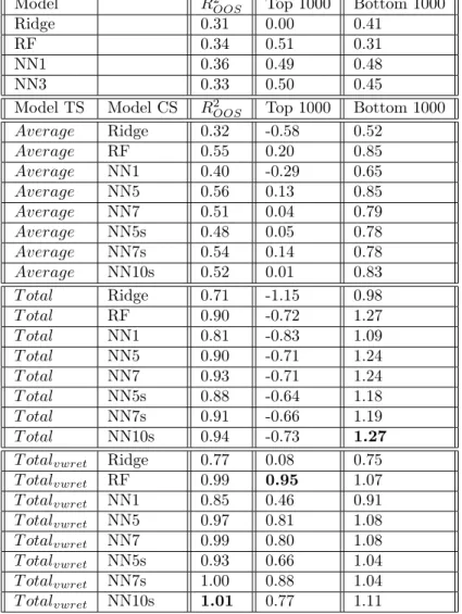
Ridge 0.31 0.00 0.41 RF 0.34 0.51 0.31 NN1 0.36 0.49 0.48 NN3 0.33 0.50 0.45 Model TS Model CS 𝑅2 𝑂𝑂𝑆 Top 1000 Bottom 1000 𝐴𝑣𝑒𝑟𝑎𝑔𝑒 Ridge 0.32 -0.58 0.52 𝐴𝑣𝑒𝑟𝑎𝑔𝑒 RF 0.55 0.20 0.85 𝐴𝑣𝑒𝑟𝑎𝑔𝑒 NN1 0.40 -0.29 0.65 𝐴𝑣𝑒𝑟𝑎𝑔𝑒 NN5 0.56 0.13 0.85 𝐴𝑣𝑒𝑟𝑎𝑔𝑒 NN7 0.51 0.04 0.79 𝐴𝑣𝑒𝑟𝑎𝑔𝑒 NN5s 0.48 0.05 0.78 𝐴𝑣𝑒𝑟𝑎𝑔𝑒 NN7s 0.54 0.14 0.78 𝐴𝑣𝑒𝑟𝑎𝑔𝑒 NN10s 0.52 0.01 0.83 𝑇 𝑜𝑡𝑎𝑙 Ridge 0.71 -1.15 0.98 𝑇 𝑜𝑡𝑎𝑙 RF 0.90 -0.72 1.27 𝑇 𝑜𝑡𝑎𝑙 NN1 0.81 -0.83 1.09 𝑇 𝑜𝑡𝑎𝑙 NN5 0.90 -0.71 1.24 𝑇 𝑜𝑡𝑎𝑙 NN7 0.93 -0.71 1.24 𝑇 𝑜𝑡𝑎𝑙 NN5s 0.88 -0.64 1.18 𝑇 𝑜𝑡𝑎𝑙 NN7s 0.91 -0.66 1.19 𝑇 𝑜𝑡𝑎𝑙 NN10s 0.94 -0.73 1.27 𝑇 𝑜𝑡𝑎𝑙𝑣𝑤𝑟𝑒𝑡 Ridge 0.77 0.08 0.75 𝑇 𝑜𝑡𝑎𝑙𝑣𝑤𝑟𝑒𝑡 RF 0.99 0.95 1.07 𝑇 𝑜𝑡𝑎𝑙𝑣𝑤𝑟𝑒𝑡 NN1 0.85 0.46 0.91 𝑇 𝑜𝑡𝑎𝑙𝑣𝑤𝑟𝑒𝑡 NN5 0.97 0.81 1.08 𝑇 𝑜𝑡𝑎𝑙𝑣𝑤𝑟𝑒𝑡 NN7 0.99 0.80 1.08 𝑇 𝑜𝑡𝑎𝑙𝑣𝑤𝑟𝑒𝑡 NN5s 0.93 0.66 1.04 𝑇 𝑜𝑡𝑎𝑙𝑣𝑤𝑟𝑒𝑡 NN7s 1.00 0.88 1.04 𝑇 𝑜𝑡𝑎𝑙𝑣𝑤𝑟𝑒𝑡 NN10s 1.01 0.77 1.11

Table 4.3: Overall 𝑅2. The first part of the table shows the performance of models trained on total returns. The second part of the table shows the performance obtained by combining different Time Series (TS) & Cross-Sectional (CS) models.

given by: 𝑅2_𝑂𝑂𝑆 = ∑︀ 𝑁 ∑︀ 𝑇(𝑟𝑖,𝑡− ˆ𝑟𝑖,𝑡)2 ∑︀ 𝑁 ∑︀ 𝑇(𝑟𝑖,𝑡)2

where 𝑟𝑖,𝑡 is ground truth returns and ˆ𝑟𝑖,𝑡 is the predicted value that is given by ˆ𝑟

′

𝑖,𝑡

+ˆ¯𝑟𝑡.

Overall 𝑅2_𝑂𝑂𝑆is presented in table 4.3. We select a subset of Cross-Sectional model for combination. Best TS model (𝑇 𝑜𝑡𝑎𝑙𝑣𝑤𝑟𝑒𝑡) and best CS model (NN10s) combine

to give the best performing model. It can be observed that when CS models are combined with 𝑇 𝑜𝑡𝑎𝑙, high cap stocks 𝑅2 _{is poor while 𝑇 𝑜𝑡𝑎𝑙}

𝑣𝑤𝑟𝑒𝑡 model’s high cap

𝑅2 is better because it is trained to predict value-weighted monthly returns.

4.4

Performance Dissection

In this section, we look at how the model performs across months, years, and indus-tries. We choose best performing model (𝑇 𝑜𝑡𝑎𝑙𝑣𝑤𝑟𝑒𝑡 + NN10s) for the analysis.

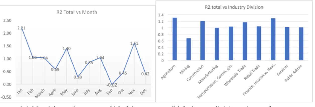
Figure 4.4, shows the year-wise performance of models. In the beginning years, the model generally performs well. There are few years specifically the 𝑅2 value goes negative (2000, 2005, 2006, 2007, 2011 & 2014). Poor performance for some years may be due to the higher volatility in the market, which makes the markets behave in unusual ways. For e.g., Dotcom bubble in 2000, the Great recession of 2007, high market volatility during 2011.

Figure 4-2, shows the monthly performance of the model aggregated over different years. September is the month-with worse performing month. The exact reason for this behavior is not known, but there is something known as the "September Effect". SnP has average decline of 0.5% since 1950 in September3_{. Similarly, 4-2 shows the}

performance across different industry divisions (based on SIC classification). The mining industry division is performing poorly compared to others.

Figure 4-1: Year-wise performance of Model

(a) Monthly performance of Model (b) Industry division wise performance

Figure 4-2: Left: Monthly performance of model aggregated over years. Right: Industry-wise performance of model.

4.5

Machine Learning Portfolio

Next, risk-premia forecast can be used for portfolio creation & the portfolios can be analyzed and used by traders. At the starting of every month, the model predictions are obtained. These return predictions are then sorted into deciles, and the portfolios are created. Stock belonging to top 10%ile are longed, and bottom 10%ile stocks are shorted.

Two types of portfolios, equally weighted and value-weighted (market capitaliza-tion is used as weights), can be constructed. For portfolios obtained from different models, the graph of log cumulative returns is shown in figure 4-3. We select some

Model Sharpe Ratio Min Ret Max Drawdown Turnover NN1 1.64 12.47 5.56 125.46 NN3 2.24 7.61 5.56 108.57 Ridge 1.37 17.00 23.87 128.06 RF 0.85 13.53 14.71 99.38 Ridge CS 1.36 16.04 22.59 131.34 RF CS 1.44 5.21 6.13 116.15 NN1 CS 2.22 8.14 5.11 119.28 NN5 CS 2.27 5.64 6.46 108.83 NN5s CS 2.26 7.09 6.62 113.14 NN7 CS 2.21 6.87 7.62 111.66 NN7s CS 2.16 9.82 5.97 112.21 NN10 CS 1.94 5.64 5.85 116.03 NN10s 2.43 7.88 5.99 113.50

Table 4.4: ML Portfolios metrics. Equal-weighted portfolios

of the best performing models from their categories for the comparison. For every portfolio, we evaluate different metrics as shown in table 4.4 and table 4.5. The met-rics include yearly Sharpe ratio, the minimum value of returns obtained in a month (Min Ret), the maximum value of drawdown (Max. Drawdown), and turnover. Only cross-sectional models are evaluated because portfolio creation is independent of the time series model. Only cross-sectional spread information is required for decile sort-ing. From the cumulative returns graph and metrics table, it can be observed that equal-weighted portfolios have a higher value of Sharpe ratio and returns. This is due to the Root Mean Square Error, which is an equal-weighted loss function used in cross-sectional models for optimization. It does not give more importance to the high capitalization stocks. Hence, we observe this behavior. For equal-weighted portfolios, the performance metrics are in order of 𝑅2 _{of models. Equal-weighted portfolio}

con-structed from NN10s CS is having the highest Sharpe ratio and cumulative returns.

4.6

Forecasting known Portfolios

The models learned can be used for forecasting returns of known portfolios. The return forecast can be obtained as follows:

(a) Equal Weighted ML Portfolios

(b) Value Weighted ML Portfolios

Figure 4-3: The graph for log cumulative returns of portfolios formed from top and bottom 10 %ile stocks. The spread in returns of long-short portfoliosis greater for Equal-weighted portfolios

Model Sharpe Ratio Min Ret Max Drawdown Turnover NN1 0.81 12.34 12.02 154.96 NN3 0.98 20.56 26.60 148.47 Ridge 0.50 11.99 12.47 134.40 RF 0.19 11.34 21.36 110.50 Ridge CS 0.50 11.71 15.44 139.09 RF CS 0.45 10.44 13.44 154.52 NN1 CS 0.78 18.24 23.60 142.91 NN5 CS 1.13 9.67 8.24 145.80 NN5s CS 1.05 14.38 19.74 142.09 NN7 1.08 13.02 19.13 143.41 NN7s 1.00 18.35 24.36 141.66 NN10 0.93 8.79 9.57 147.36 NN10s 1.16 15.44 20.49 145.89

Table 4.5: ML Portfolios metrics. Value(cap)-weighted portfolios

ˆ 𝑟𝑡+1𝑝 =

∑︁

𝑤𝑖* ˆ𝑟𝑖,𝑡+1

where ˆ𝑟𝑝_𝑡+1 is forecasted portfolio returns, 𝑤𝑖 are the portfolio weights & ˆ𝑟𝑖,𝑡+1 is the

returns predicted.

The portfolios used for analysis are double sorted(3x2) book-to-market, momen-tum, investment & size. They are constructed using a similar methodology used in Fama French data library(French (2013)). The 𝑅_𝑝𝑓2 for different portfolios are in table 4.6. 𝑅2 _{is calculated as follows:} 𝑅2_𝑝𝑓 = ∑︀ 𝑇(𝑟 𝑝 𝑡 − ˆ𝑟 𝑝 𝑡)2 ∑︀ 𝑇(𝑟 𝑝 𝑡 − 𝑟 𝑝 𝑚)2

Where 𝑟𝑝_𝑡 is portfolio return at time t, ˆ𝑟_𝑡𝑝 is predicted value of return and 𝑟𝑝_𝑚 is mean historic return. Portfolios are more predictable than stocks due to averaging of noise present in stock returns. Hence, we observe higher 𝑅2. From the results, the Random Forest method performs best on a large number of portfolios followed by 5 Hidden Layer Neural Network with skip connections. From the earlier results, it can be observed that RF and NN5s achieve higher 𝑅2 _{for high cap (Top 1000) stocks,}

Pf NN1 NN3 Ridge RF Ridge CS RF CS NN1 CS NN5 CS NN7 CS NN5s CS NN10s CS SMB 1.06 0.88 -0.03 0.44 -0.38 0.75 0.54 0.75 1.33 2.20 1.81 HML 1.87 1.03 1.98 1.05 2.04 1.38 2.37 1.45 2.00 2.33 1.70 BB 1.72 1.25 0.70 1.36 3.32 4.38 3.40 3.53 3.94 3.56 3.72 BS 1.27 0.57 1.24 1.42 4.90 4.52 4.07 4.18 4.28 4.08 4.30 MS 0.97 0.51 0.32 1.40 2.26 2.89 2.28 2.65 2.74 2.08 2.49 MB 0.40 0.24 -1.53 -0.21 -1.63 1.52 -1.08 0.77 0.81 -0.54 0.60 SS 0.65 0.49 -1.27 0.04 -1.37 1.76 -0.82 1.02 1.06 -0.29 0.84 SB 0.07 -0.09 -1.86 -0.55 -1.96 1.19 -1.41 0.44 0.48 -0.88 0.27 CMA 0.05 1.16 0.29 -0.22 -0.99 -0.13 -0.03 1.25 1.96 3.13 2.78 BB -0.20 0.23 -2.77 0.04 -4.19 1.18 -1.28 0.52 0.74 0.01 0.66 BS 0.87 0.05 -0.21 1.54 2.25 3.70 2.69 3.11 3.09 2.38 2.67 MS 0.91 0.24 0.17 1.17 2.37 3.02 2.19 2.59 2.66 1.92 2.42 MB 0.00 0.19 -1.49 -0.55 -3.65 -0.41 -2.43 -0.94 -0.68 -1.44 -0.66 SS 3.39 3.57 1.94 2.86 -0.14 2.99 1.04 2.48 2.73 2.00 2.75 SB 0.69 0.88 -0.79 0.15 -2.94 0.28 -1.72 -0.25 0.02 -0.74 0.03 UMD 1.47 0.03 2.56 4.31 2.45 5.09 -0.82 -0.60 -0.81 -1.38 -1.36 BB 0.17 0.44 -1.06 -0.90 -2.37 0.07 -1.07 -0.12 -0.02 -0.38 0.05 BS 7.57 5.77 7.13 7.33 10.39 9.52 9.26 9.58 9.98 9.33 9.35 MS 5.00 3.44 4.00 5.24 9.25 9.39 8.87 9.21 9.40 8.73 8.93 MB -0.82 -0.48 -2.91 -0.30 -3.33 1.41 -1.03 0.55 0.63 -0.02 0.46 SS -0.80 -0.45 -2.88 -0.28 -3.31 1.43 -1.01 0.57 0.65 0.00 0.49 SB -0.83 -0.48 -2.91 -0.31 -3.34 1.41 -1.03 0.55 0.63 -0.02 0.46

Table 4.6: Results of forecasting known portfolios. The naming of portfolios is as follows: XY, X refers to the first variable (book-to-market, momentum, invest-ment) sort it can be Small (S), Middle(M), Big(B) and Y refers to the second variable (size) sorting, it can be Small(S) and Big(B). CMA refers to Conservative Minus Ag-gressive. UMD refers to Up Minus Down. HML is High Minus Low, and SMB is Small Minus Big.

Chapter 5

Explainability

In this chapter, we analyze the Machine Learning models learned and try to explain them.

The models that are learned for risk-premia prediction are used by investors to make portfolios. The investors would prefer to know the inputs/features driving the output before making investment decisions. Most of the machine learning models are functionally black boxes. Hence, the need to explain Machine Learning models.

In general, Ridge Regression models can easily be analyzed due to their linear nature. In comparison, Random Forests and Deep Networks suffers from the problem of black-box nature. As discussed earlier, Ridge Regression models do not perform as good as Deep Models. Hence, people use Deep Models, and we try to explain Deep Models.

We use a recently developed method called Local Interpretable Model-Agnostic Explanations (LIME) (Ribeiro et al. (2016)) for explaining the predictions of the Black Box model. It is a model agnostic technique that can approximate the decision boundary near a data point.

5.1

Local Interpretable Model-Agnostic Explanations

LIME explains the behavior of the model around the instance that is being analyzed or predicted. It is a model agnostic method. To figure out what inputs contribute to

the prediction of an input 𝑥, it perturbs input 𝑥 and calculates the prediction for each perturbed input. Once the perturbed dataset is ready, a weighted ridge regression model is trained where the weights are decided by the distance of perturbed data point to original data point. The trained regression coefficients give the interpretable contribution of each feature in prediction output for input 𝑥. The above procedure can be done for any black-box model. This makes LIME model-agnostic.

For our analysis, we take the best performing deep model Neural network 10 + skip connections (NN10+s CS). The network comprises of 10 hidden layers. It makes it challenging to analyze the transformations and calculate the feature importance directly. A similar analysis can also be done for all black-box models.

5.1.1

Local Feature Importance

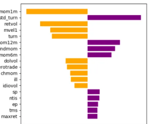
For every test point, the feature importance can be calculated using LIME. The fea-ture importance can be considered as the contribution of each feafea-ture in the predicted output. An example of top features and their importance for a data point is shown in figure 5.1.1. Short term reversal (mom1m) is the highest contributing feature for this particular example, and it is negatively correlated to cross-sectional returns predicted. Out of all the features used for training network, only a few of them contributed to the output, and their importance is shown. Similarly, for all test points, feature importance can be obtained.

5.1.2

Global Feature Importance

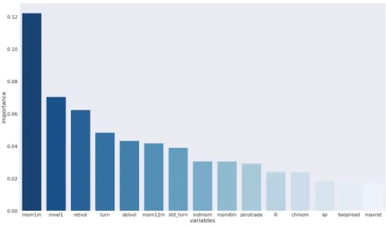
Once the feature importance for each data point is obtained, it can be aggregated to obtain global feature importance. In our case, we take the average of absolute values to obtain global feature importance. Figure 5.1.2 shows the global feature importance for top 15 features out of 94(firm-specific) & 8(macroeconomic) features. Again, very few features contribute to the output out of all features.

Like global feature importance, the year-wise feature importance can also be cal-culated by aggregating the feature importance for all the data points for a particular

Figure 5-1: LIME feature importance for a data point. Only top few features are plotted.

year. The year-wise feature importance is shown in figure 5-3. From the heatmap, we can observe the set of the important variables remain consistent. In general, short term reversal (mom1m) stays an important feature across all years; in later years, other features have also become important compared to earlier years.

5.1.3

Importance Histogram

The previous analysis gives us the results of overall feature importance. It does not tell us anything about the relationship between input features and the output variables. To find out the relationship between the inputs and output, the histogram of the LIME coefficients(feature importance) is plotted for all the data points. The histograms for some features are shown in figure 5-4. The presence of data on both sides of zero (for e.g., 6-months momentum, max return) implies that particular factor affects returns in both ways positively and negatively based on some conditions. It throws light on the non-linear nature of the Deep Models that cannot be learned by the linear models. Histogram of the factors that are not important is concentrated around 0, e.g., leverage. Most of the relationships learned by the model between factor and risk-premia are consistent with the literature findings except in a few cases.

Figure 5-2: LIME feature importance aggregated over all data points. Top 15 features are plotted.

∙ mom1m: Short term reversal (mom1m) is known to be correlated negatively to returns (Cakici and Topyan (2014)). The histogram of mom1m shows majorly negative coefficients.

∙ mom12m: Momentum 12 months (mom12m) is known to be correlated posi-tively to returns (Figelman (2007)). The histogram of mom1m shows majorly positive coefficients.

∙ indmom: If a particular industry is doing well, companies belonging to that industry group must likely be doing well. The histogram of industry momentum shows majorly positive coefficients.

∙ mvel1 (size): Small-cap stocks generally have high growth. High growth stocks have positive risk premia 1_.

1

∙ retvol: Return volatility is known to be both positively and negatively related (Harvey and Lange (2015)). The histogram obtained for retvol have data on both sides of zero. Hence it is both positively and negatively related.

∙ turn: High turnover stocks are known to have smaller risk premia (Hu (1997)). The histogram shows a negative relation between turnover and returns.

∙ std_turn: Volatility of Liquidity should be negatively related to the risk pre-mia (Pereira and Zhang (2010)) . The histogram obtained shows a positive relation. For this factor, it can be observed that the relationship learned is not consistent with the literature. When the explanation gives much importance to std_turn, the investor can be aware of it and then decide whether to actually trust the model.

Overall, any black-box model can be analyzed using LIME. Looking at an inter-pretable explanation of a prediction gives confidence to any investor using the model. It also gives information about the essential variables that affect risk-premia.

Figure 5-3: LIME feature importance aggregated over data points year-wise. We can observe only few features are consistently important across different years.

(a) Momentum 1 month (b) Momentum 6 months (c) Momentum 12 months

(d) Industry Momentum (e) Return Volatility (f) Size

(g) Max Return (h) Turnover (i) Zero Trading Days

(j) Illiquidity (k) Std dev of Turnover (l) Leverage

Figure 5-4: Histogram of LIME coefficients for different features. It can be observed that for more essential features, histograms have long tails. The majority behavior of different features can be observed, e.g., negative coefficients of the mom1m histogram implies: short term reversion (mom1m) is negatively correlated to the output.

Chapter 6

Conclusion

Our results show that macroeconomic and firm factors have information about risk-premia that can be used for its estimation. Machine Learning models can be used to learn this relationship.

In this work, we trained different ML models and observed that, in general, Deep Networks outperform linear ML models. We explored some of the problems associated with Deep Networks like performance degradation with increasing layers and lack of interpretability. Inspired from Deep learning literature, we modified the architecture of the network that led to the training of deeper networks with better performance. We also modeled the risk-premia using two different networks that had dual benefits: it solved the non-stationary problem of returns, and it decoupled learning returns into two independent components: Time Series and Cross-Sectional. The models learned were evaluated robustly on yearly, monthly, and industry basis. We also constructed portfolios that can be used by investors for trading and evaluated them on different metrics.

We also explored the black-box nature of Deep Networks and used the meth-ods existing in the literature to explain the model predictions. Investors can use the explainability analysis to get confidence in model predictions before making any investment decisions. We also get an idea about the different variables that have predictive power. Overall, this work captures the non-linear interaction between fac-tors and risk-premia. Our work gives a robust model that can be used by industries

and individual investors for portfolio construction and for understanding the factors related to risk-premia.

Appendix A

Name Description Name Description

dp Dividend-price ratio PERMITMW New Private Housing Permits, Midwest (SAAR) ep Earnings-price ratio PERMITS New Private Housing Permits, South (SAAR) bm Book-to-market ratio PERMITW New Private Housing Permits, West (SAAR) ntis Net equity expansion AMDMNOx New Orders for Durable Goods

tbl Treasury bill rate AMDMUOx Unlled Orders for Durable Goods tms Term spread BUSINVx Total Business Inventories

dfy Default spread ISRATIOx Total Business: Inventories to Sales Ratio svar Stock variance M1SL M1 Money Stock

dy Dividend yield ratio M2SL M2 Money Stock de Dividend payout ratio M2REAL Real M2 Money Stock

ltr Long term rate AMBSL St. Louis Adjusted Monetary Base dfr Default return spead TOTRESNS Total Reserves of Depository Institutions infl Consumer price index NONBORRES Reserves Of Depository Institutions cay Consumption. wealth, income ratio BUSLOANS Commercial and Industrial Loans

lty Long term yeild REALLN Real Estate Loans at All Commercial Banks RPI Real Personal Income NONREVSL Total Nonrevolving Credit

W875RX1 Real personal income ex transfer receipts CONSPI Nonrevolving consumer credit to Personal Income DCERA Real personal consumption expenditures S&P 500 S&P’s Common Stock Price Index: Composite CMRMTSPLx Real Manu. and Trade Industries Sales S&P: indust S&P’s Common Stock Price Index: Industrials RETAILx Retail and Food Services Sales S&P div yield S&P’s Composite Common Stock: Dividend Yield INDPRO IP Index S&P PE ratio S&P’s Composite Common Stock: P-E Ratio IPFPNSS IP: Final Products and Nonindustrial Supplies FEDFUNDS Eective Federal Funds Rate

IPFINAL IP: Final Products (Market Group) CP3Mx 3−Month AA Financial Commercial Paper Rate IPCONGD IP: Consumer Goods TB3MS 3-Month Treasury Bill

IPDCONGD IP: Durable Consumer Goods TB6MS 6-Month Treasury Bill IPNCONGD IP: Nondurable Consumer Goods GS1 1-Year Treasury Rate IPBUSEQ IP: Business Equipment GS5 5-Year Treasury Rate IPMAT IP: Materials GS10 10-Year Treasury Rate

IPDMAT IP: Durable Materials AAA Moody’s Seasoned Aaa Corporate Bond Yield IPNMAT IP: Nondurable Materials BAA Moody’s Seasoned Baa Corporate Bond Yield IPMANSICS IP: Manufacturing (SIC) COMPAPFFx 3-Month Commercial Paper Minus FEDFUNDS IPB51222S IP: Residential Utilities TB3SMFFM 3-Month Treasury C Minus FEDFUNDS IPFUELS IP: Fuels TB6SMFFM 6-Month Treasury C Minus FEDFUNDS CUMFNS Capacity Utilization: Manufacturing T1YFFM 1-Year Treasury C Minus FEDFUNDS HWI Help-Wanted Index for United States T5YFFM 5-Year Treasury C Minus FEDFUNDS HWIURATIO Ratio of Help Wanted/No. Unemployed T10YFFM 10-Year Treasury C Minus FEDFUNDS CLF16OV Civilian Labor Force AAAFFM Moody’s Aaa Corporate Bond Minus FEDFUNDS CE16OV Civilian Employment BAAFFM Moody’s Baa Corporate Bond Minus FEDFUNDS UNRATE Civilian Unemployment Rate EXSZUSx Switzerland / U.S. Foreign Exchange Rate UEMPMEAN Average Duration of Unemployment (Weeks) EXJPUSx Japan / U.S. Foreign Exchange Rate UEMPLT5 Civilians Unemployed - Less Than 5 Weeks EXUSUKx U.S. / U.K. Foreign Exchange Rate

UEMP5TO14 Civilians Unemployed for 5-14 Weeks EXCAUSx Canada / U.S. Foreign Exchange Rate UEMP15OV Civilians Unemployed−15 Weeks & Over WPSFD49207 PPI: Finished Goods

UEMP15T26 Civilians Unemployed for 15-26 Weeks WPSFD49502 PPI: Finished Consumer Goods UEMP27OV Civilians Unemployed for 27 Weeks and Over WPSID61 PPI: Intermediate Materials CLAIMSx Initial Claims WPSID62 PPI: Crude Materials

PAYEMS All Employees: Total nonfarm OILPRICEx Crude Oil, spliced WTI and Cushing USGOOD All Employees: Goods-Producing Industries PPICMM PPI: Metals and metal products CES1021000001 All Employees: Mining and Logging: Mining CPIAUCSL CPI : All Items

USCONS All Employees: Construction CPIAPPSL CPI : Apparel MANEMP All Employees: Manufacturing CPITRNSL CPI : Transportation DMANEMP All Employees: Durable goods CPIMEDSL CPI : Medical Care NDMANEMP All Employees: Nondurable goods CUSR0000SAC CPI : Commodities SRVPRD All Employees: Service-Providing Industries CUSR0000SAD CPI : Durables USTPU All Employees: Trade, Transportation & Utilities CUSR0000SAS CPI : Services

USWTRADE All Employees: Wholesale Trade CPIULFSL CPI : All Items Less Food USTRADE All Employees: Retail Trade CUSR0000SA0L2 CPI : All items less shelter USFIRE All Employees: Financial Activities CUSR0000SA0L5 CPI : All items less medical care USGOVT All Employees: Government PCEPI Personal Cons. Expend.: Chain Index CES0600000007 Avg Weekly Hours : Goods-Producing DDURRG Personal Cons. Exp: Durable goods AWOTMAN Avg Weekly Overtime Hours : Manufacturing DNDGRG Personal Cons. Exp: Nondurable goods AWHMAN Avg Weekly Hours : Manufacturing DSERRG Personal Cons. Exp: Services

HOUST Housing Starts: Total New Privately Owned CES0600000008 Avg Hourly Earnings : Goods-Producing HOUSTNE Housing Starts, Northeast CES2000000008 Avg Hourly Earnings : Construction HOUSTMW Housing Starts, Midwest CES3000000008 Avg Hourly Earnings : Manufacturing HOUSTS Housing Starts, South MZMSL MZM Money Stock

HOUSTW Housing Starts, West DTCOLNVHFNM Consumer Motor Vehicle Loans Outstanding PERMIT New Private Housing Permits (SAAR) DTCTHFNM Total Consumer Loans and Leases Outstanding PERMITNE New Private Housing Permits, Northeast (SAAR) INVEST Securities in Bank Credit at All Commercial Banks

Table A.2: Definitions of macro variables used in Time Series models. First 15 variables are obtained from Welch and Goyal (2008) and remaining are obtained from Fred-MD dataset McCracken and Ng (2016)

absacc Absolute accruals mom36m 36−month momentum acc Working capital accruals mom6m 6−month momentum aeavol Abnormal earnings announcement volume ms Financial statement score age # years since first Compustat coverage size Size

agr Asset growth mve_ia Industry−adjusted size baspread Bid−ask spread nincr Number of earnings increases beta Beta operprof Operating profitability betasq Beta squared orgcap Organizational capital

bm_annual Book−to−market pchcapx_ia Industry adjusted % change in capital expenditures bm_ia Industry−adjusted book to market pchcurrat % change in current ratio

cash Cash holdings pchdepr % change in depreciation

cashdebt Cash flow to debt pchgm_pchsale % change in gross margin − % change in sales cashpr Cash productivity pchquick % change in quick ratio

cfp Cash−flow−to−price ratio pchsale_pchinvt % change in sales − % change in inventory cfp_ia Industry−adjusted cash−flow−to−price ratio pchsale_pchrect % change in sales − % change in A/R chatoia Industry−adjusted change in asset turnover pchsale_pchxsga % change in sales − % change in SG&A chcsho Change in shares outstanding pchsaleinv % change sales-to-inventory

chempia Industry−adjusted change in employees pctacc Percent accruals chinv Change in inventory pricedelay Price delay

chmom Change in 6−month momentum ps Financial statements score chpmia Industry−adjusted change in profit margin quick Quick ratio

chtx Change in tax expense rd R&D increase

cinvest Corporate investment rd_mve R&D to market capitalization convind Convertible debt indicator rd_sale R&D to sales

currat Current ratio realestate Real estate holdings depr Depreciation / PP&E retvol Return volatility divi Dividend initiation roaq Return on assets divo Dividend omission roavol Earnings volatility dolvol Dollar trading volume roeq Return on equity dy Dividend to price roic Return on invested capital ear Earnings announcement return rsup Revenue surprise egr Growth in common shareholder equity salecash Sales to cash ep Earnings to price saleinv Sales to inventory gma Gross profitability salerec Sales to receivables grCAPX Growth in capital expenditures secured Secured debt grltnoa Growth in long−term net operating assets securedind Secured debt indicator herf Industry sales concentration sgr Sales growth hire Employee growth rate sin Sin stocks idiovol Idiosyncratic return volatility SP Sales to price

ill Illiquidity std_dolvol Volatility of liquidity (dollar trading volume) indmom Industry momentum std_turn Volatility of liquidity (share turnover) invest Capital expenditures and inventory stdacc Accrual volatility

lev Leverage stdcf Cash flow volatility

lgr Growth in long−term debt tang Debt capacity/firm tangibility maxret Maximum daily return tb Tax income to book income mom12m 12−month momentum turn Share turnover

mom1m 1−month momentum zerotrade Zero trading days

Table A.1: Definitions of 94 firm specific variables used in models. The detailed description of variables is available in Green et al. (2017).

Bibliography

Breiman, Leo (2001), “Random forests.” Mach. Learn., 45, 5–32, URL https://doi.org/10.1023/A:1010933404324.

Cakici, Nusret and Kudret Topyan (2014), Short-Term Reversal, 91–103. Palgrave Macmillan US, New York, URL https://doi.org/10.1057/97811373590707.

Chen, Luyang, Markus Pelger, and Jason Zhu (2019), “Deep learning in asset pricing.” Available at SSRN 3350138.

Feng, Guanhao, Jingyu He, and Nicholas G Polson (2018), “Deep learning for pre-dicting asset returns.” arXiv preprint arXiv:1804.09314.

Figelman, Ilya (2007), “Stock return momentum and

rever-sal.” The Journal of Portfolio Management, 34, 51–67, URL

https://jpm.pm-research.com/content/34/1/51.

French, Kenneth R (2013), “Fama french-data library.” Cited on, 193.

Green, Jeremiah, John R. M. Hand, and X. Frank Zhang (2017), “The Char-acteristics that Provide Independent Information about Average U.S. Monthly Stock Returns.” The Review of Financial Studies, 30, 4389–4436, URL https://doi.org/10.1093/rfs/hhx019.

Gu, Shihao, Bryan Kelly, and Dacheng Xiu (2018), “Empirical asset pricing via ma-chine learning.” Working Paper 25398, National Bureau of Economic Research, URL http://www.nber.org/papers/w25398.

Gu, Shihao, Bryan Kelly, and Dacheng Xiu (2020), “Autoencoder asset pricing mod-els.” Journal of Econometrics.

Harvey, Andrew and Rutger-Jan Lange (2015), “Modeling the interactions between volatility and returns.”

He, Kaiming, Xiangyu Zhang, Shaoqing Ren, and Jian Sun (2016), “Identity mappings in deep residual networks.” In European conference on computer vision, 630–645, Springer.

Hu, Shing-yang (1997), “Trading turnover and expected stock returns: The trading frequency hypothesis and evidence from the tokyo stock exchange.” Available at SSRN 15133.

Huang, Gao, Zhuang Liu, Laurens Van Der Maaten, and Kilian Q Weinberger (????), “Densely connected convolutional networks.” In Proceedings of the IEEE conference on computer vision and pattern recognition, 4700–4708.

Kelly, Bryan, Seth Pruitt, and Yinan Su (2017), “Some characteristics are risk expo-sures, and the rest are irrelevant.” Unpublished Manuscript, University of Chicago. McCracken, Michael W and Serena Ng (2016), “Fred-md: A monthly database for

macroeconomic research.” Journal of Business & Economic Statistics, 34, 574–589. Nakagawa, Kei, Takumi Uchida, and Tomohisa Aoshima (2018), “Deep factor model.”

In ECML PKDD 2018 Workshops, 37–50, Springer.

Pereira, Joao Pedro and Harold H Zhang (2010), “Stock returns and the volatility of liquidity.” Journal of Financial and Quantitative Analysis, 1077–1110.

Ribeiro, Marco Tulio, Sameer Singh, and Carlos Guestrin (2016), “"why should I trust you?": Explaining the predictions of any classifier.” In Proceedings of the 22nd ACM SIGKDD International Conference on Knowledge Discovery and Data Mining, San Francisco, CA, USA, August 13-17, 2016, 1135–1144.

Simonyan, Karen, Andrea Vedaldi, and Andrew Zisserman (2013), “Deep inside con-volutional networks: Visualising image classification models and saliency maps.” arXiv preprint arXiv:1312.6034.

Springenberg, Jost Tobias, Alexey Dosovitskiy, Thomas Brox, and Martin Ried-miller (2014), “Striving for simplicity: The all convolutional net.” arXiv preprint arXiv:1412.6806.

Sundararajan, Mukund, Ankur Taly, and Qiqi Yan (2017), “Axiomatic attribution for deep networks.” arXiv preprint arXiv:1703.01365.

Welch, Ivo and Amit Goyal (2008), “A comprehensive look at the empirical perfor-mance of equity premium prediction.” The Review of Financial Studies, 21, 1455– 1508.

Zeiler, Matthew D and Rob Fergus (2014), “Visualizing and understanding convolu-tional networks.” In European conference on computer vision, 818–833, Springer.