HAL Id: halshs-00553130
https://halshs.archives-ouvertes.fr/halshs-00553130
Preprint submitted on 6 Jan 2011
HAL is a multi-disciplinary open access archive for the deposit and dissemination of sci-entific research documents, whether they are pub-lished or not. The documents may come from teaching and research institutions in France or
L’archive ouverte pluridisciplinaire HAL, est destinée au dépôt et à la diffusion de documents scientifiques de niveau recherche, publiés ou non, émanant des établissements d’enseignement et de recherche français ou étrangers, des laboratoires
Endogenous timing game with non-monotonic reaction
functions
Grégoire Rota-Graziosi, Magnus Hoffmann
To cite this version:
Grégoire Rota-Graziosi, Magnus Hoffmann. Endogenous timing game with non-monotonic reaction functions. 2011. �halshs-00553130�
CERDI, Etudes et Documents, E 2010.17 Document de travail de la série Etudes et Documents E 2010.17
Endogenous timing game with non‐monotonic reaction functions.
Magnus Hoffmann* and Grégoire Rota Graziosi‡ *: University of Magdeburg, Department of Economics, Institute of Public Economics, Universitaetsplatz 2, 39108 Magdeburg, Germany. Email: [email protected] ‡: CERDI‐CNRS, Université d'Auvergne, 65 boulevard François Mitterrand, 63000 Clermont‐Ferrand, France Email: gregoire.rota_graziosi@u‐clermont1.fr 27 Avril 2010
April 27, 2010
Endogenous timing game with non-monotonic reaction functions.
Abstract
The aim of this paper is to generalize the endogenous timing game proposed by Hamilton and Slutsky (1990) to cases where the reaction functions are non-motononic, as for instance in the literature on contest. Following the taxonomy of social dilemma provided by Eaton (2004) we consider several pos-sible situations depending on the nature of interactions (plain complementarity or plain substituability and strategic complementarity or strategic substitutability). Under the assumptions of the existence and the uniqueness of the Nash and Stackelberg equilibria, we highlight the presence of a first-mover advantage or a second-mover incentive only depending on the nature of cross-effects in players’ payoff functions and the slopes of their reaction functions at the Nash equilibrium of the static game. These properties allow us to determine rigorously the Subgame Perfect Nash Equilibrium (SPNE) in the ten studied situations. We establish under which conditions on the nature of interactions a leader emerges at the SPNE.
Keywords: endogenous timing game; first-mover advantage; second-mover incentive; Subgame Perfect Nash Equilibrium.
JEL classification: C72; D43; L13.
Magnus Hoffmann* and Grégoire Rota Graziosi‡
*: University of Magdeburg, Department of Economics,
Institute of Public Economics, Universitaetsplatz 2, 39108 Magdeburg, Germany. Email: magnus.hoff[email protected]
‡: CERDI-CNRS, Université d’Auvergne,
Mail address: 65 boulevard François Mitterrand, 63000 Clermont-Ferrand, France Email: [email protected]
1
Introduction
The seminal article of Hamilton and Slutsky (1990) endogeneizes the Stackelberg leadership in a duopoly game. This model is important since it provides a simple formalization of the trade-off between pre-commitment and flexibility. The considered commitment consists in moving before the others and corresponds to a “pure unconditional commitment” in Schelling’s termi-nology. Amir (1995) completes Hamilton and Slutsky (1990) by establishing the necessity of an additional condition, that is the monotonicity of each payoff in the other player’s actions.
Several developments of Hamilton and Slutsky (1990) have been proposed in the literature. For instance, Sadanand and Sadanand (1996) consider demand uncertainty in this model. In order to deal with the multiple equilibria issue, which may appear van Damme and Hurkens (1999) introduce the notion of risk-dominance as defined by Harsanyi and Selten (1988). Amir and Stepanova (2006) use the tool of supermodularity to make the minimum of assumptions. They distinguish three possible cases depending on the slope of the reaction functions (positive or negative for both players or positive for one, negative for the other). They establish general conditions on the demand functions to highlight first- or second-mover advantage and then to solve the endogenous timing game. However, these developments and others restrict themselves to situations where the reaction functions are monotonic.
Even though the assumption of monotonic reaction functions encompasses often the main specifications proposed in the IO literature, there are important exceptions. For example Bulow, Geanakoplos, and Klemperer (1985a) show that for the case of the constant elasticity of demand in Cournot duopoly, the reaction functions are non-monotonic. The same holds for the best responses of duopolists in the endogenous-timing duopoly model examined by Maskin and Tirole (1988). In an infinite horizon framework the dynamic reaction functions in a price competition model also exhibit non-monotonicity. Adner and Zemsky (2005) examine a model of technology innovation in different markets in a Cournot-framework. In their model the emergence of competition between technologies alters the shape of the demand functions for products in two different markets in a manner which induces non-monotonic best responses.
other fields, as for instance international trade or public economics, where commitments are an important issue too. For example, Syropoulos (1994) shows the (non) equivalence of policy instruments (quotas and tarriffs) in the context of non-cooperative policy games with endoge-nous timing. In this framework the tariff reaction functions of a country exhibits strategic substitutability and complementarity, contingent on the other country’s decision on it’s tariff. Dixit (1987) and Baik and Shogren (1992) analyze a contest for an exogenous rent between two players whom reaction functions are increasing and then decreasing. This game is neither super-modular nor subsuper-modular since the players’ actions are strategic complements for the “favorite”, while they are strategic substitutes for the “underdog”1 at the Nash Equilibrium. Finally, we
can also mention the recent work of Stengel (2010), who compares the leader and follower payoff in a symmetric duopoly game without the assumption of monotonic reaction functions. This author concludes that the follower payoff is either higher than the leader payoff, or lower than in the simultaneous game.
In this paper, we propose a generalization of Hamilton and Slutsky (1990) by considering non-monotonic reaction functions. Following Eaton (2004) who provides a useful taxonomy of social dilemma, we consider ten possible situations depending on the nature of interactions (plain complementarity or plain substitutability and strategic complementarity or strategic substitutability). Admitting the existence and the uniqueness of the Nash and Stackelberg equilibria, we highlight the presence of a first-mover advantage or a second-mover incentive only depending on the nature of cross-effects in players’ payoff functions and the slopes of the reaction functions at the Nash equilibrium of the static game. These properties are then sufficient to determine the Subgame Perfect Nash Equilibrium(s) (SPNE) of the endogenous timing game proposed by Hamilton and Slutsky (1990). By doing this, we then extend the taxonomy of Eaton (2004) in determining the SPNE(s) in each studied case. The rest of this paper is organized as follows: section 2 precises the assumptions of Hamilton and Slutsky (1990) and derives some properties of the payoff functions; section 3 establishes the SPNE(s) of the endogenous timing game; section 4 concludes.
1 Dixit (1987) defines the “favorite” (respectively the “underdog”) as the player who has a probability to
2
Model
First, we present our assumptions. Secondly, we consider the three basic games (the static game and the two Stackelberg ones) and give a sufficient partial ranking of the equilibrium values. Third, we identify the presence of a first-mover advantage or a second-mover incentive.
2.1
Assumptions
The (continuous) payoff functions are given by Πi(x
i, xj), where xi ∈ Xi (respectively xj ∈ Xj)
is the strategy of player i (j) defined over a nonempty compact interval of the real line.2 We
make the assumption that player i’s payoff functions is concave in her own action and monotone in the other player’s action. Thus, existence of a Nash equilibrium (NE) is assured. Following Eaton and Eswaran (2002), we define plain interactions, more precisely plain complements (PC) and plain substitutes (PS).
Definition 1 The game exhibits plain complements (plain substitutes) for player i if
∀ (xi, xj)∈ Xi× Xj, ∂Πi(x i, xj) ∂xj ≡ Π i j(xi, xj) > 0 (< 0) .
The notion of plain interactions is very close to this of spillovers, but it appears more precise than the latter. The necessary condition given by Amir (1995) is then equivalent to the assumption that the property of PC or PS holds for any values of xi and xj. Following Bulow,
Geanakoplos, and Klemperer (1985b), we will also use the notion of strategic complementarity (SC) or strategic substituabiliy (SS). Let denote by ∂2Π∂xi∂xji(xi,xj) ≡ Πi
ij(xi, xj) the second cross
derivative of the payoff function for player i. We have SC (respectively SS) for player i if Πi
ij(xi, xj) > 0 (respectively Πiij(xi, xj) < 0). Since we consider non-monotonic best responses
the property of SC and SS may vary for a player, contingent on the strategies chosen by both players.3 We therefore will define the property of SC or SS at the Nash Equilibrium (NE) of
the static game.
2 The action x
i may be for instance quantity in Cournot duopoly, price in Bertrand duopoly, effort in a
rent-seeking game or tax rate in a model of tax competition.
Definition 2 At the Nash Equilibrium of the static game, defined by xN
≡¡xNi , xNj
¢
, player i regards strategic complements (strategic substitutes) if
∀ (xi, xj)∈ Xi× Xj, ∂2Πi(xi, xj) ∂xi∂xj ¯ ¯ ¯ ¯ xN ≡ Πiij ¡ xNi , x N j ¢ > 0 (< 0) .
These definitions allow us to encompass several different settings, which are considered by Eaton (2004). For instance, the classic version of the Cournot duopoly is a game of PS and SS, while the Bertrand duopoly with differentiated goods is a game of PC and SC. The model of private provision of a public good proposed by Bergstrom, Blume, and Varian (1986) exhibits PC and SS for players and a formalization of defense expenditure among enemy countries would be a game of PS and SC (see Eaton (2004)). However, we will also consider some mixed situations going beyond the taxonomy proposed by Eaton (2004) and getting closer to the seminal work of Hamilton and Slutsky (1990). For instance, our results may be applied to some particular and influential frameworks, as the model of Singh and Vives (1984), or to the contest games usually used in the rent seeking literature. Singh and Vives (1984), which is considered in Hamilton and Slutsky (1990) discuss an asymmetric case, where two firms in a differentiated duopoly market can only make two types of binding contracts with consumers, a price contract and a quantity contract. In the case where both firms decide to make different decisions regarding the nature of the contract, we obtain a game of PC and PS for one firm (which chooses the price contract) and a game of PS and SS for the other firm (which chooses a quantity contract). An important application of our results would be the literature, which uses the Contest Succes Function.4 Indeed, since we allow for non-monotonic best responses the property of SC and SS may vary for a player, contingent on the strategies chosen by both players. In the case of rent seeking, as provided by Dixit (1987), player i’s best response function increases in xj for lower values of xj, and decreases in xj for higher values of xj. In other terms,
each contestant regards actions as SC or SS depending on her effort and the opponent’s effort. Existence and uniqueness of the the Nash and Stackelberg equilibriums usually involve several restrictions on the payoff functions. In order to remain as general as possible, we make the following assumptions
Assumption 1
(i) The Nash equilibrium of the simultaneous game is unique. (ii) The equilibrium of the Stackelberg games exists and is unique.
The first assumptions guarantees that our definition of SC, or SS respectively, is unique for each player in the static game. A sufficient condition for the uniqueness of the Stackelberg equilibrium is the concavity of the Stackelberg leader’s payoff function Πi¡x
i, xFj (xi)
¢
, where xFj (xi) is the reaction function of player j. More formally, we assume for the rest of the paper
that d2Πi¡xi, xFj (xi) ¢ dx2 i < 0. (1)
Given Assumption (1), in particular the assumption of uniqueness regarding the Stackelberg-equilibrium, we know that the sign of the slope of players’ best response functions at the NE are identical to the sign of the slope of the follower’s best response function in the Stackelberg equilibrium.
2.2
A sufficient partial ranking of the equilibrium values at the three
basic games
We consider three basic games, denoted by ΓN, ΓS1 and ΓS2, which respectively correspond to the static game and to the two Stackelberg games. Let denote by ¡xN
i , xNj
¢
the Nash equi-librium values of the static game, and ¡xL
i, xFj
¡ xL
i
¢¢
the equilibrium values of the Stakelberg equilibrium, where player i leads. We have
⎧ ⎪ ⎨ ⎪ ⎩
xNi ≡ arg maxxi∈XiΠi(xi, xj)
xNj ≡ arg maxxj∈XjΠ j(x
j, xi) .
(2)
The Stackelberg equilibrium is determined by backward induction. We have:
xFj (xi)≡ arg max xj∈XjΠ
j(x
and xLi ≡ arg max xi∈XiΠ i¡x i, xFj (xi) ¢ . (4)
Given the optimizing behavior in the basic games (expressions 2, 3 and 4), we are now in the position to establish some partial rankings of the levels of agents’ actions at the different equilibrium, which would be sufficient for our principal result. We then have:5
Lemma 1 Under Assumption (1), we have: ∀ (i, j) ∈ {1, 2}2 and i 6= j, xNj > xLj ⇔ ½ Πiij ¡ xNi , xNj ¢ > 0 Πji (xj, xi) < 0 or ½ Πiij ¡ xNi , xNj ¢ < 0 Πji(xj, xi) > 0, (5) and xNj < xLj ⇔ ½ Πi ij ¡ xN i , xNj ¢ > 0 Πji (xj, xi) > 0 or ½ Πi ij ¡ xN i , xNj ¢ < 0 Πji(xj, xi) < 0. (6)
Proof. See Appendix A.1.
This Lemma compares the NE’s level with this choosen by the leader. The obtained rankings result from the concavity of the objective function of the leader given in (1). Let consider for instance the case of SC for player i at the NE and PS for player j. By definition, the leader anticipates how the follower would react to a change in her action with respect to the NE values. When player j leads, it is in her own interest to induce a reduction of the action of the other player (i), since this action is a PS for player j. Due to the property of SC for player i, the leader (player j) knows that by reducing her action she initiates the other player to do the same. That is the reason why we obtain in this case: xLj < xNj . Similar reasonings apply for
the other situations.
2.3
First-mover advantage and second-mover incentive
We now compare the payoffs in the three basic games (ΓN, ΓS1 and ΓS2), which will give us
the opportunity of detecting potential first-mover (second-mover) advantages or first-mover (second-mover) incentives. We define these notions as follows
Definition 3 (i) Player i has a first-mover advantage (a second-mover advantage) if her equi-librium payoff in the Stackelberg game in which she leads, denoted by ΓSi, is higher (lower) than
5 For the rest of the paper, we pose xF
in the Stackelberg game in which she follows ¡ΓSj¢.
(ii) Player i has a first-mover incentive (a second-mover incentive) if her equilibrium payoff in the Stackelberg game in which she leads (she follows), denoted by ΓSi ¡ΓSj¢, is higher than in
the static game ¡ΓN¢.
From Lemma (1) and Definition 3, we can state that:
Lemma 2 Under Assumption (1), we have
• Player i has a first-mover advantage if
— Actions are SC at the NE for player i and they induce PC for one player and PS for the other,
— Or if actions are SS at the NE for player i and they are PC or PS for both players. More formally, we have
Πi¡xLi, xFj ¢> Πi¡xFi , xLj¢⇔ ½ Πi ij ¡ xN i , xNj ¢ > 0 Πi j(xi, xj) Πji(xj, xi) < 0 or ½ Πi ij ¡ xN i , xNj ¢ < 0 Πi j(xi, xj) Πji (xj, xi) > 0.
• Player i has a second-mover incentive if
— Actions are SC at the NE for player i and they induce PC for one player and PS for the other„
— Or if actions are SS at the NE for player i and they are PC or PS for both players. Equivalently, Πi¡xNi , xNj ¢> Πi¡xFi , xLj¢⇔ ½ Πi ij ¡ xN i , xNj ¢ > 0 Πi j(xi, xj) Πji (xj, xi) > 0 or ½ Πi ij ¡ xN i , xNj ¢ < 0 Πi j(xi, xj) Πji (xj, xi) < 0.
Proof. see Appendix A.2.
The preceding Lemma takes into account the non-monotonicity of the reaction functions, since it relies only on the sign of the second cross derivatives at the NE of the static game. The intuition is the following. If, for instance, we have SC for player i at the NE and a game of PC for player j, then, given Lemma 1, we know that the Stackelberg leader will increase xj
compared to the NE-level. The effect of this on player i’s payoff is twofold. There is a direct effect, the payoff effect, which is positive (negative), given that is a game of PC (PS) for player i. And there is an indirect effect, the strategic effect, which causes xi to increase (decrease) given
that player i regards xj as SC (SS). However, the indirect effect, caused by the increase of xj on
player i’s reaction is unambiguous, since player i will maximize her payoff by moving towards her best response function. The net effect on player i’s payoff is positive if it is a game of PC for
player i, and negative if it is a game of PS for player i. Therefore, in this setting, player i has a second-mover incentive in the former case and a second-mover disincentive,6 or equivalently,
a first-mover advantage, in the latter one.
Note, that once we know whether plain interactions (PS or PC) have a similar effect for both players, we only need to know whether a player’s best response function is in- or decreasing to identify a first-mover advantage or a second-mover incentive. For instance, in the classical Cournot Duopoly game (with PS) as well as in the private provision of public goods framework (with PC) we establish a first mover advantage for both players. Moreover, in the case where the cross-effects in the payoff functions are of different signs, a game with SS for player i and SC for player j at the NE, player j will always have a first-mover advantage and player j a second-mover incentive. The reason for this is that player i, whether she increases or decreases xi as a Stackelberg leader compared to the NE, will always choose a point in the strategy space
that lies inside the Pareto-superior set, defined as
PS ≡©x1, x2| Πi(xi, xj) > Πi(xNi , x N
j )∀ i, j = 1, 2 and i 6= j
ª .
Player j, on the other hand, always chooses a point in the strategy space outside PS.
3
Resolving the endogenous timing game
The issue of endogenous timing is examined according to the extended game with observable delay proposed by Hamilton and Slutsky (1990). This game, denoted by ˜Γ, allows players to choose non-cooperatively and simultaneously their timing decision in a preplay stage either as soon as (early) or as late as possible (late). Their decision is announced by the players subsequently. The players choose then their action according to their timing decision to which they are committed. If both players decide to play at the same time (whether early or late), the static game ¡ΓN¢ is played. If player i chooses to move early and player j chooses to move
late, the Stackelberg game ¡ΓSi¢ where player i leads is played. The extended game ³Γ˜´ has 6 See expression (15) in Appendix A.2.
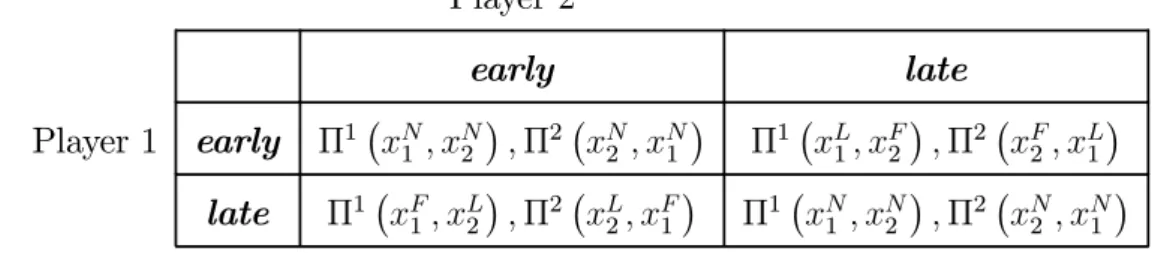
the following reduced normal form:
Table 1: Normal form of the extended game
Player 2 early late Player 1 early Π1¡xN 1 , xN2 ¢ , Π2¡xN 2 , xN1 ¢ Π1¡xL 1, xF2 ¢ , Π2¡xF 2, xL1 ¢ late Π1¡xF1, xL2 ¢ , Π2¡xL2, xF1 ¢ Π1¡xN1 , xN2 ¢ , Π2¡xN2 , xN1 ¢
The solution of the game ³Γ˜´is equivalent to the solution of the leadership problem. There is no leader if both players choose the same timing decision; a leader emerges when they choose complementary roles. Under our assumptions, the solution of the timing game can be directly explained by the nature of the interactions among the two players at the Nash equilibrium of the static game only. We obtain the following Theorem:
Theorem 1 Under Assumption (1), we have:
• If payoff functions exhibit similar plain interactions ¡Πij(xi, xj) Π j
i(xj, xi) > 0
¢ , then
1. The SPNEs are the two Stackelberg outcomes, if players’ strategies are SC at the NE.
2. The SPNE is the outcome of the static game, if players’ strategies are SS at the NE. 3. The SPNE is the outcome of the Stackelberg game ¡ΓSi¢ where player i for whom
actions are SS at the NE will act as a Stackelberg leader and player j for whom actions are SC at the NE will act as a Stackelberg follower.
• If payoff functions exhibit opposite plain interactions ¡Πi
j(xi, xj) Πji (xj, xi) < 0
¢ , then
1. The SPNE is the outcome of the static game, if players’ strategies are SC at the NE. 2. The SPNEs are the two Stackelberg outcomes, if players’ strategies are SS at the NE. 3. The SPNE is the outcome of the Stackelberg game ¡ΓSi¢ where player i for whom
actions are SS at the NE will act as a Stackelberg follower and player j for whom actions are SC at the NE will act as a Stackelberg leader.
Proof. See Appendix A.3.
Theorem (1) shows that the SPNE(s) is contingent on the nature of plain and strategic interactions. For instance if plain interactions are of the same sign for both players, it is sufficient for a sequential move game to emerge as an SPNE, if one of the players regards
actions as SC. The sufficient condition if the signs of plain interactions differ is that one of the players regards actions as SS. The reason for this is that a leader, thus the outcome of a Stackelberg game, would only emerge at the SPNE if at least one best response function lies in the Pareto-superior set. Only in this case we have a second-mover incentive for at least one player.
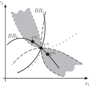
Figures 1 and 2 provide a graphical illustration of our result. In both figures player 1 exhibits SC and player 2 SS. Figure 1 represents the cases when plain interactions are similar. The bold lines represent the non-monotonic reaction functions of player 1 and 2. The dashed (dotted) lines represent the iso-payoff-curves of the players when the game exhibits PS (PC) for both players. In the case of PS (PC) the Pareto-superior set PS, represented by the grey surface,
lies to the south-west (north-east) of the NE. Thus, a sequential move game will emerge as a SPNE if at least one of the players regards actions as a SC, here player 1.
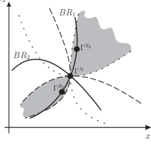
If the signs of plain interactions differs the opposite holds. In figure 2 the dashed (dotted) lines represent the iso-payoff curves of the players when the game exhibits PS (PC) for player 1 and PC (PS) for player 2 and the grey surface to the south-east (north-west) represents PS. Hence, at least one player has to regard actions as a SS in order to guarantee a Stackelberg outcome as the SPNE of the extended game (here, player 2).
Figure 2: Opposite plain interactions.
Given Theorem (1), we can also state the following Corollary.
Corollary 2 Under Assumption (1), we have:
(i) If the unique SPNE of the extended game is the outcome of a Stackelberg game, then the SPNE Pareto-dominates the simultaneous game and the other Stackelberg game.
(ii) If the SPNEs of the extended game are the outcomes of the two Stackelberg games, then both SPNEs Pareto-dominate the static game, but can not be ranked in a Pareto sense among each other.
(iii) If the unique SPNE of the extended game is the simultaneous move game, then the outcomes of the three basic games can not be ranked in a Pareto sense.
Proof. Immediate
It is worth mentioning that in the case of multiplicity of SPNE (PC and SS or PS and SC), several authors as van Damme and Hurkens (1999), van Damme and Hurkens (2004) or Amir and Stepanova (2006) use the notion of risk-dominance. However, this notion may not be applied without specifying the payoff functions. For instance, van Damme and Hurkens (1999) or Amir and Stepanova (2006) use linear demand functions in a duopoly context.
An immediate illustration of our results is the analysis of contest provided by Dixit (1987) and Baik and Shogren (1992). In a two-players contest for an exogenous rent, these authors define the “favorite” and the “underdog” through the probability of winning the contest at the Nash equilibrium of the static game: the “favorite” (respectively the “underdog”) has a probability superior (respectively inferior) to one half. We can easily establish that this contest
corresponds to a game of PS for both players where for one player, in fact the “underdog”, appropriation efforts are SS, while for the other, the “favorite”, efforts are SC. For instance, let consider a logit Contest Success Function, denoted by p (xi, xj) .We have
p (xi, xj) =
fi(xi)
fi(xi) + fj(xj)
,
where f0
i(xi) > 0 > fi00(xi)by assumption. This is also the probability of winning the exogenous
rent R for player i depending on her effort xi and the effort of the other player (xj). The payoff
of players are
Πi(xi, xj) = p (xi, xj) R− xi and Πj(xj, xi) = (1− p (xi, xj)) R− xj.
We note that
Πiij(xi, xj) = pij(xi, xj) R =−Πjij(xj, xi) ,
Thus, the strategic interactions among players can never be of the same sign. Moreover, we have pij(xi, xj) = [fi(xi)− fj(xj)] fi0(xi) fj0(xj) [fi(xi) + fj(xj)] 3 > 0 ⇔ fi(xi) > fj(xj)⇔ p (xi, xj) > 1 2.
Thus, the Stackelberg outcome where the “underdog” leads is the SPNE of the commitment game as Baik and Shogren (1992) established it, since players’ actions are SS at the NE for the “underdog” and plain interactions are of the same sign for both players (PS).
4
Conclusion
We generalize the Hamilton and Slutsky’ game of commitment by taking into account the non-monotonicity of the reaction functions. We consider several situations depending on the nature of interactions among two players. The underlying games may then be neither supermodular nor submodular. By signing the slopes of the reaction functions at the Nash equilibrium of
the static game, we are able to provide a partial ranking of the equilibrium values of players’ actions. This ranking allows us to establish the presence of a first-mover advantage or a second-mover incentive, which in turn yield to determine the SPNE. We conclude that a leader and obviously a follower emerge at the SPNE(s) if for at least one of the players actions are strategic complements (strategic substitutes) at the Nash Equilibrium of the static game and the cross-effects in the payoff functions are of the same (different) sign(s) for both players.
References
Adner, R., and P. Zemsky (2005): “Disruptive technologies and the emergence of competi-tion,” The Rand Journal of Economics, 36(2), 229—254.
Amir, R. (1995): “Endogenous timing in two-player games: a counterexample,” Games and Economic Behavior, 9(2), 234—237.
Amir, R., and A. Stepanova (2006): “Second-mover advantage and price leadership in Bertrand duopoly,” Games and Economic Behavior, 55(1), 1—20.
Baik, K. H.,and J. F. Shogren (1992): “Strategic behavior in contests: comment,” American Economic Review, 82(1), 359—362.
Bergstrom, T., L. Blume, and H. Varian (1986): “On the private provision of public goods,” Journal of Public Economics, 29(1), 25—49.
Bulow, J. I., J. D. Geanakoplos, and P. D. Klemperer (1985a): “Holding idle capacity to deter entry,” The Economic Journal, 95(377), 178—182.
(1985b): “Multimarket oligopoly: strategic substitutes and complements,” Journal of Political Economy, 93(3), 488—511.
Dixit, A. (1987): “Strategic behaviour in contests,” American Economic Review, 77(5), 891—98. Eaton, B. C. (2004): “The elementary economics of social dilemmas,” Canadian Journal of
Economics, 37(4), 805—829.
Eaton, B. C., and M. Eswaran (2002): Applied Microeconomic Theory. Edward Elgar Pub-lishing.
Hamilton, J. H., and S. M. Slutsky (1990): “Endogenous timing in duopoly games: Stack-elberg or cournot equilibria,” Games and Economic Behavior, 2(1), 29—46.
Harsanyi, J. C., and R. Selten (1988): A general theory of equilibrium selection in games. MIT Press, Cambridge, MA.
Maskin, E., and J. Tirole (1988): “A Theory of Dynamic Oligopoly, II: Price competition, kinked demand curves, and Edgeworth cycles,” Econometrica, 56(3), 571—599.
Sadanand, A., and V. Sadanand (1996): “Firm scale and the endogenous timing of entry: a choice between commitment and flexibility,” Journal of Economic Theory, 70(2), 516—530. Singh, N., and X. Vives (1984): “Price and quantity competition in a differentiated duopoly,”
RAND Journal of Economics, 15(4), 546—554.
Stengel, B. v. (2010): “Follower payoffs in symmetric duopoly games,” Games and Economic Behavior, Forthcoming.
Syropoulos, C. (1994): “Endogenous timing in games of commercial policy,” Canadian Jour-nal of Economics, 27(4), 847—64.
van Damme, E., and S. Hurkens (1999): “Endogenous Stackelberg leadership,” Games and Economic Behavior, 28(1), 105—129.
A
Appendix
A.1
Proof of Lemma 1 (a partial ranking)
Let define the function Ψi(xi) as
Ψi(xi) ≡ Πii ¡ xi, xFj(xi)¢+ Πij ¡ xi, xFj(xi)¢ dx F j (xi) dxi . (7)
This function corresponds to the first derivative of the leader payoff function: Ψi(xi) = ∂Πi
i(xi,xFj(xi))
∂xi . For x
L i,
we obtain the FOC of the leader, that is Ψi
¡ xL
i
¢
= 0. Under Assumption (1ii) we have Ψ0
i(xi) < 0. • If Πjij ¡ xN j , xNi ¢
> 0, actions are SC for the player j at the Nash equilibrium, or equivalently dx
F j(xi) dxi > 0
at xi= xNi (the reaction function of player j is increasing in xi at the Nash equilibrium). From (7), we
have Ψi¡xNi ¢ = Πii¡xNi , xFj(xNi )¢+ Πij¡xNi , xFj(xNi )¢ dx F j (xi) dxi = Πij¡xNi , xFj(xNi )¢ dx F j (xi) dxi , since Πi i ¡ xN i , xFj(xNi ) ¢ = Πi i ¡ xN i , xNj ¢
= 0. We now consider two situations depending on the presence of PC or PS.
— If Πi
j(xi, xj) > 0, from preceding we obtain
Ψi¡xNi ¢ > 0 = Ψi¡xLi ¢ , since dx F j(xi)
dxi > 0. The decreasing of Ψi(.) in xi involves
Ψi¡xNi
¢
> Ψi¡xLi
¢
⇔ xNi < xLi. (8)
— In constrast, PS for player i¡Πij(xi, xj) < 0¢involves
Ψi ¡ xNi ¢< Ψi ¡ xLi¢⇔ xNi > xLi. (9) • If Πjij ¡ xN j , xNi ¢ < 0, then we have dx F j(xi)
dxi < 0 at the Nash equilibrium. The two cases are then
— If Πi j(xi, xj) > 0, we deduce that Ψi ¡ xNi ¢< Ψi ¡ xLi¢⇔ xNi > xLi. (10) — If Πi j(xi, xj) < 0, we have Ψi¡xNi ¢ > Ψi¡xLi ¢ ⇔ xNi < xLi. (11) ¤
A.2
Proof of Lemma 2 (First-mover advantage and second-mover
incentive)
By definitions of the Stackelberg and the Nash equilibria, we have Πi¡xLi, xFj ¡xiL¢¢ > Πi¡xi, xFj (xi)¢ > Πi¡xN i , xFj ¡ xN i ¢¢ = Πi¡xN i , xNj ¢ , (12)
where the first inequality results from the leader’s maximization program, and the second from the specification of xito xNi . The leader of the Stackelberg game always has a payoff level superior or equal to this obtained at
the Nash equilibrium. In other terms, players always have a first-mover incentive.
We determine under which conditions in terms of PC, PS, SC or SS player i will have a first-mover advantage or a second-mover incentive .
A.2.1 First-mover advantage
From the maximization’s program given in (4), we know that player i’s payoff as a Stackelberg leader is Πi¡xLi, xFj¢ > Πi¡xNi , xNj ¢= max
xi
Πi¡xi, xNj
¢
> Πi¡xFi , xNj ¢, (13)
where the first inequality results from (12) and the second from the definition of the Nash maximization program. The existence of a first-mover advantage may be reduced to determine the conditions such that the following inequality holds: Πi¡xF i , xNj ¢ > Πi¡xF i , xLj ¢ . (14)
This inequality only emerges if
• The cross-effect in the player i’s payoff function is positive (Πij(.) > 0) and xNj > xLj, which, given
Lemma (1), is only consistent with ½ Πi ij ¡ xN i , xNj ¢ > 0 Πji(xi, xj) < 0 or ½ Πi ij ¡ xN i , xNj ¢ < 0 Πji(xi, xj) > 0.
• The cross-effect in the player i’s payoff function is negative (Πi
j(.) < 0) and xNj < xLj, which, given
Lemma (1), is equivalent to ½ Πiij¡xNi , xNj ¢> 0 Πji(xi, xj) > 0 or ½ Πiij¡xNi , xNj ¢< 0 Πji(xi, xj) < 0.
We remark that a player who has a first-mover advantage has also a second-mover dis-incentive, formally defined as
Πi¡xNi , xNj ¢> Πi¡xFi , xLj¢. (15)
A.2.2 Second-mover incentive
From (3), we know that
Πi¡xFi , xLj¢= max
xi
Πi¡xi, xLj¢ > Πi
¡
xNi , xLj¢. (16)
To highlight a second-mover incentive, we have to establish conditions for the following inequality: Πi¡xNi , xLj
¢
> Πi¡xNi , xNj
¢
. (17)
This inequality only emerges if
• The cross-effect in the player i’s payoff function is positive (Πi
j(.) > 0) and xNj < xLj, which, given
Lemma (1), is only consistent with ½ Πi ij ¡ xN i , xNj ¢ > 0 Πji(xi, xj) > 0 or ½ Πi ij ¡ xN i , xNj ¢ < 0 Πji(xi, xj) < 0.
• The cross-effect in the player i’s payoff function is negative (Πi
j(.) < 0) and xNj > xLj, which, given
Lemma (1), is only consistent with ½ Πi ij ¡ xN i , xNj ¢ > 0 Πji(xi, xj) < 0 or ½ Πi ij ¡ xN i , xNj ¢ < 0 Πji(xi, xj) > 0.
A.2.3 Payoffs’ ranking
From (12), (13), (14), (16), (17) and (15) we deduce the following rankings of the player i’s payoff function at the equilibrium of the three basic games depending on the existence of a first-mover advantage or a second-mover incentive:
Player i has a first-mover advantage ⇔ Πi¡xLi, xFj¢> Πi¡xNi , xNj ¢> Πi¡xFi , xLj¢, (18) and
Player i has a second-mover incentive ⇔ ½ Πi¡xF i , xLj ¢ > Πi¡xN i , xNj ¢ Πi¡xLi, xFj¢> Πi¡xNi , xNj ¢. (19) ¤
A.3
Proof of Theorem 1 (Subgame Perfect Nash Equilibria)
A player always has a first-mover incentive: Πi¡xL i, xFj
¢
> Πi¡xN i , xNj
¢
, ∀i ∈ {1, 2} (see expression 12). In order to determine the SPNE, we use the results in Lemma (2) and may compare the payoff levels when the country follows and when it plays simultaneously (Πi¡xF
i, xLj¢ ≶ Πi ¡ xN i , xNj ¢ ). • If payoff functions exhibit similar plain interactions³Πi
j(xi, xj) Πji(xj, xi) > 0
´ , 1. SC at the NE for both players: Πi
ij
¡ xN
i , xNj
¢
> 0 for (i, j) ∈ {1, 2}. Both players have a second-mover incentive (see Lemma 2). Since both have also a first-second-mover incentive, we deduce that the SPNE are the two Stackelberg outcomes: if a player chooses to play early, the other prefers to move late; if a player chooses to play late, the other prefers to play early.
2. SS at the NE for both players: Πiij¡xNi , xNj ¢ < 0 for (i, j) ∈ {1, 2}. Both players have a first-mover advantage (see Lemma 2) and a second-first-mover disincentive: Πi¡xN
i , xNj ¢ > Πi¡xF i , xLj ¢ (see expression 18). The SPNE are then the Nash outcome: moving early is a strictly dominant strategy for both players.
3. SC for player 2 and SS for player 1 (at the NE): Π2 12 ¡ xN 2, xN1 ¢ > 0 > Π1 12 ¡ xN 1 , xN2 ¢ . Lemma (2) establishes that player 1 has a first-mover advantage, while player 2 has a second-mover incentive. Combining with the first-mover incentive for both players, we have:
½ Π1¡xL 1, xF2 ¢ > max©Π1¡xN 1, xN2 ¢ , Π1¡xF 1, xL2 ¢ª Π2¡xF 2, xL1 ¢ > Π2¡xN 2, xN1 ¢ . (20)
The SPNE is the outcome of the Stackelberg game where player 1 leads and player 2 follows. • If payoff functions exhibit opposite plain interactions³Πi
j(xi, xj) Πji(xj, xi) < 0
´ ,
1. SC at the NE for both players. From Lemma (2) both players have a first-mover advantage and a second-mover disincentive (see expression 18). Thus, the dominant strategy for both players is to play early. The unique SPNE is then the outcome of the simultaneous move game.
2. SS at the NE for both players. Both players have a second-mover incentive (see Lemma 2). Since both have also a first-mover incentive, we deduce that the SPNE are the two Stackelberg outcomes. 3. SC for player 2 and SS for player 1 (at the NE): Π2
12 ¡ xN 2 , xN1 ¢ > 0 > Π1 12 ¡ xN 1, xN2 ¢ . From Lemma (2), we know that player 1 has a second-mover incentive and player 2 has a first-mover advantage. The SPNE is then the outcome of the Stackelberg game where player 1 follows and player 2 leads.¤