A modified Lax-Wendroff correction for wave propagation in media described by Zener elements

(1)

Geophys. J . Int. (1997) 131,381-386

A

modified Lax-Wendroff correction for wave propagation in media

described by Zener elements

J. 0

Blanch' and

J.

0.

A. Robertsson2**

Defence Research Establishment, Enkopingsuagen 126, S-172 90 Stockholm, Sweden 'Institute of Geophysics, Swiss Federal Institute of Technology, Zurich, Switzerland

Accepted 1997 July 4. Received 1997 July 2; in original form 1996 December 12

S U M M A R Y

A modified Lax-Wendroff correction for wave propagation in attenuating and dispersive media described by Zener elements is presented. As opposed to the full correction, this new technique is explicit and offers large computational savings. The technique may be applied to a wide variety of hyperbolic problems. Here, the concept is illustrated for wave propagation in visco-acoustic media.

Key words: attenuation, electromagnetic modelling, finite-difference methods, seismic modelling, viscoelasticity.

I N T R O D U C T I O N

Explicit finite-difference schemes are commonly employed to solve wave-propagation problems. The temporal accuracy of such schemes can be increased by employing a Lax- Wendroff correction (e.g. Lax & Wendroff 1964; Dablain 1986; Gustafsson, Sjoberg & Abrahamsson 1988; Sei 1991). In the literature, this technique is also referred to as a modified scheme or, somewhat ambiguously, a compact scheme. The approach yields drastic improvements in numerical characteristics of finite-difference schemes (Dablain 1986).

During the last decade, convolutional formulations of con- stitutive relations to model wave propagation in attenuating and dispersive media have been employed extensively (e.g. Emmerich & Korn 1987; Carcione, Kosloff & Kosloff 1988; Kunz & Luebbers 1993; Robertsson, Blanch & Symes 1994). By employing an array of Zener elements (standard linear solids in visco-acoustics), an essentially arbitrary quality factor, Q, versus frequency, f , behaviour can be obtained (Blanch, Robertsson & Symes 1995). The quality factor, Q

=

%(c2))/

&m(c2)), where c(f) is the phase velocity as a function of frequency, roughly corresponds to the number of wavelengths that a wave can propagate before its amplitude decays by a factor of e-n (White 1992). Unfortunately, as we will show in this paper, the full Lax-Wendroff correction is generally not a good candidate for this class of scheme.

We present a modified Lax-Wendroff correction with numerical properties as good as or even better than the full correction. Additionally, the computational cost in terms of calculations per gridpoint of the new scheme is only increased by roughly 30 per cent. The technique may be applied to various hyperbolic problems, including acoustic, elastic and electromagnetic wave propagation. Here, we illustrate the

*

Now a t Schlumberger Cambridge Research, Cambridge, UK.

method for the l-D viscoacoustic case, where we increase the accuracy in time from second to fourth order.

L A X - W E N D R O F F F I N I T E - D I F F E R E N C E SCHEME

To increase the temporal accuracy of a finite-difference scheme without expanding the temporal stencil, a Lax-Wendroff correction may be used (Lax & Wendroff 1964). For a function u( t, x) described by a hyperbolic system of partial differential equations, the temporal accuracy of a staggered (Virieux 1986) second-order accurate finite-difference approximation,

uAr = ( u " ~ " ~ - un- '/')/At, may be increased by expressing u , , , ~

through spatial derivatives, since

where At denotes the discretization in time and II denotes the

discrete time level.

In particular, the following equations describe visco-acoustic wave propagation in one dimension:

where p is the pressure, u the velocity, p the density and n ( t ) is the relaxation function (Robertsson et al. 1994). Wave propagation in real-Earth media may be modelled through an array of L Zener elements (Blanch et al. 1995):

(3)

(2)

382 J . 0. Blanch and J. 0. A . Robertsson

attenuation strength, tuL is a stress-relaxation time defining the frequency for the maximum attenuation for element 1, and H ( t ) is the Heaviside function (Blanch et ul. 1995). Introducing a memory variable, r, for the special case of L = 1 yields (Robertsson et al. 1994):

(4) 1

- ( r

+

KTU,,)

The full Lax-Wendroff corrections for increasing a second- order accurate approximation of eq. (4) to fourth-order accuracy are

1 1 T l

- K T ~ U , , - K - ~ p , ~ ~

T U P T u

The full 0 ( 4 , 4 ) scheme is obtained by adding the correction terms in eq. ( 5 ) and approximating the first-order spatial derivatives by fourth-order accurate centred differences, and the spatial derivatives in the correction terms by second-order accurate approximations. Here, 0 ( 4 , 4 ) denotes a scheme fourth-order accurate in both time and space.

An alternative approach is to use eq. (2) to calculate the correction terms:

I

The factor

n,c

contains one term with a Heaviside function and one term with a Dirac function. Since the Dirac function dominates the Heaviside function, we neglect the Heaviside function in the following approximation, which will effectively yield the full Lax-Wendroff correction for an acoustic equation, that is a wave equation without dispersion and attenuation. Hence, concentrating on wave propagation,

( 7 )

Again, the convolution is eliminated by introducing a memory variable. A so-called pseudo-0(4, 4 ) scheme can be obtained by adding the correction terms as described in eq. (7).

The Lax-Wendroff corrections derived above are strictly only applicable to homogeneous media. To construct a Lax-

Wendroff correction which is strictly applicable to heterogeneous media is a simple task (e.g. Sei & Symes 1994). The main purpose of this paper is not to explain the Lax-Wendroff correction itself, but to show that in the case of a medium described by a set of relaxation mechanisms (Zener elements) a large part of the full Lax-Wendroff correction can be neglected. In other words, the purpose of the paper is to make the use of a Lax-Wendroff correction feasible for media described by Zener elements.

N U M E R I C A L P R O P E R T I E S

The correction terms for the full 0 ( 4 , 4 ) scheme (eq. 5 ) are considerably more computationally expensive than the ‘pseudo’ corrections in eq. (7). This would become particularly cumber- some in higher dimensions. Moreover, the terms with spatial second derivatives have to be implemented implicitly for the scheme to obtain the desired accuracy and hence require an even larger amount of computational effort. Additionally, the same terms in eq. (5) would lead to an extra stability condition, since they correspond to a heat equation which grows exponentially in time. Hence certain combinations of At, T and za would lead to an ill-posed problem.

A thorough stability analysis of schemes of the same type as the pseudo-0(4,4) scheme is presented by Blanch (1995). The stability criterion for the pseudo-0(4,4) scheme is

(8) K ( 1 + t ) At 1

J

T

G

~

where A x is the spatial discretization and D is the dimension in space. The value of the left-hand side of eq. (8) is commonly referred to as the Courant number. Note that we have increased the stability limit by a factor of 7/6 compared to the analogous scheme that is second-order accurate in time [referred to as the 0 ( 2 , 4 ) scheme; Robertsson et al. (1994)l.

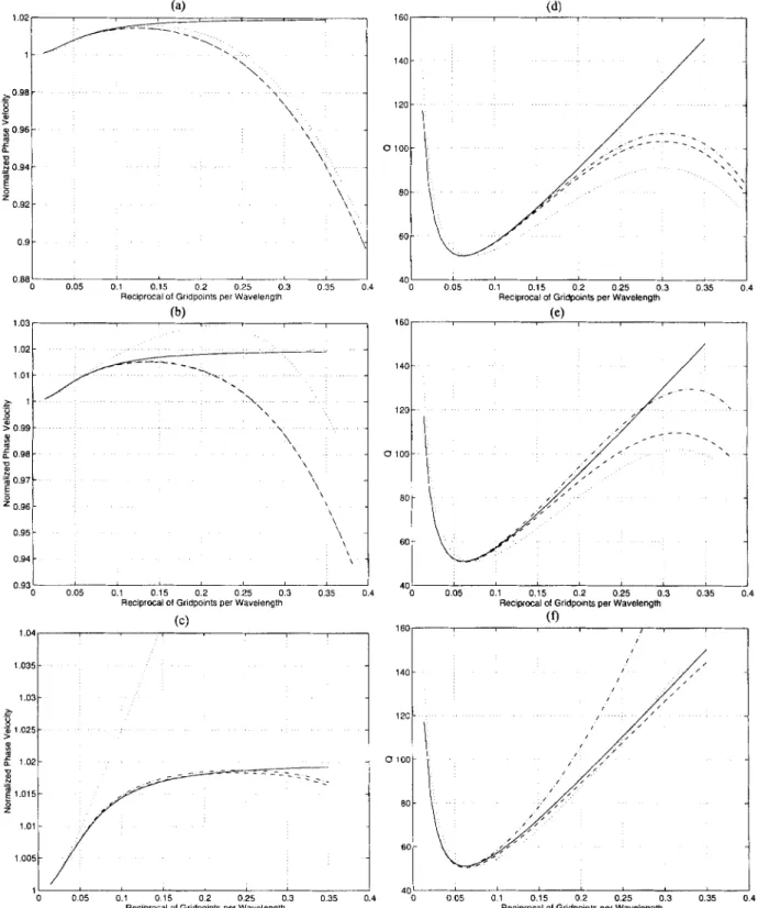
We derived the numerical dispersion relations for the 0(2,4), the 0(4,4) and the pseudo-0(4,4) schemes. Fig. 1 shows a set

of dispersion and attenuation curves for a medium with one Zener element with T = 0.04 and q = At/ta = 0.4 for different fractions of the maximum stable Courant number. The phase velocity of the pseudo-0(4,4) scheme is nearly identical to that-of the 0 ( 4 , 4 ) scheme (Figs la-c), clearly displaying the characteristic 0( 4,4) behaviour. The pseudo-0(4,4) scheme is superior overall to the 0(2,4) scheme. In particular, close to the stability limit, an almost perfect fit to the analytical curve is obtained for the pseudo-0(4,4) scheme. In contrast to the 0(2,4) scheme, an important quality of the pseudo-0(4,4) scheme is that the phase velocity is rarely overestimated (for most values of q and t ) . This has practical consequences for the picking of first-breaks, for instance. Although numerical attenuation generally has less severe influence on the simulation results compared to numerical dispersion, the pseudo-0(4,4) scheme displays the best performance (Figs Id-f).

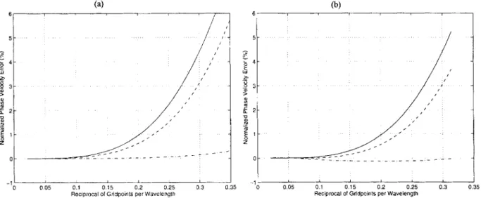
In Fig. 2 we illustrate the insensitivity of the dispersion characteristics on q for the pseudo-0(4,4) scheme. Fig. 2(a) shows the difference between the numerical and the analytical dispersion for a wide range of 4. Even though a value of 4 = 100 is unrealistically large and therefore of little interest, the curves are very similar (such large values of q correspond to peak attenuation frequencies of the Zener elements far above the simulation-source frequency range). Fig. 2( b) shows the corresponding curves for the attenuation. The error is higher for a value of q = 100, but overall the curves are similar.

(3)

A mod$ed Lax- Wendrofl correction 383 1 0 2 1 - a o 9 8 -

.

5

---

- _ '\ \ ' \ \ $ 0 9 6 - m c u s 0 9 4 - b m 0 92

Reciprocal of Gridpoints per Wavelength

088

I

- 0 0 0 5 0 1 0 1 5 0 2 0 2 5 0 3 0 3 5 0 4 (b) 1 0 3 \ \ \\ \

,

\ \ -\\

-

\ 0 9 5 1 '\

-1

$ 0 9 6 - m c u s 0 9 4 - b m 0 92 0941 \ \ \\ \

,

\ \ -\\

-

\ '\\

{

1

0 93' I 0 0 0 5 0 1 0 1 5 0 2 0 2 5 0 3 0 3 5 0 4 Reciprocal of Gridpoints per Wavelength

1035 140 120- 0 100- 80 60 2. 1 0 2 5 1 - - -

1

8 1 0 2 - D - - - -- --- -- ~ ~ - N 1 0 1 5 - 1 0 1 -

.;IT-

1005 - 1 0 005 0 1 0 1 5 0 2 0 2 5 0 3 0 3 5 0 4

I / ,

0 005 0 1 0 1 5 0 2 0 2 5 0 3 0 3 5 0 4

12a

I

/

40

0 0 0 5 0 1 0 1 5 0 2 0 2 5 0 3 0 3 5 0 4

Reciprocal 01 Gridpoinis per Wavelengm

Figure 1. Dispersion (a-c) and attenuation (d-f) curves for an analytical solution (solid), the pseudo-0(4,4) scheme (dashed), the 0 ( 4 , 4 ) scheme (dash-dotted) and the 0 ( 2 , 4 ) scheme (dotted). T = 0.04. q = 0.4. Courant numbers: 33 per cent of stability limit (a and d), 66 per cent of stability limit ( b and e) and 99 per cent of stability limit (c and f ) .

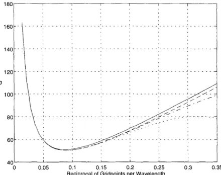
The value of 7 is approximately 2/Q (Blanch et al. 1995).

Fig. 3 shows the dispersion errors, which illustrate the and (b). insensitivity of the dispersion characteristics on 7 for the

pseudo-0(4,4) scheme. Fig. 3(a) corresponds to the acoustic case of z = 0, whereas in Fig. 3(b), a 7 of 0.3 (Q z 6) is used.

Curves corresponding to the same fraction of maximum stable

Courant number display similar characteristics in Figs 3(a)

Since the scheme is relatively insensitive to both 4 and z, it is possible to derive a general wavefield sampling criterion. For the pseudo-0(4,4) scheme, five gridpoints per wavelength are required to achieve less than 1 per cent numerical

(4)

384 J. 0. Blanch and J . 0. A . Robertsson 4 -

-

2? E 3 5 - tii

5

3 - >"

:

2 -

-

>. - ~ 2 5 - m c - 0 z 1 - 0 5 - 0 - 0 0 5 0 1 0 1 5 0 2 0 2 5 0 3 035

Figure 2. Dispersion (a) and attenuation (b) error curves in per cent for the pseudo-0(4,4) scheme for various values of q at 80 per cent of the stability limit. z = 0.04. q = 0.001 (solid), q = 0.5 (dashed), q = 100 (dash-dotted).

0 0 5 0 1 0 1 5 0 2 0 2 5 0 3 035 Reciprocal 01 Gridpoints per Wavelength

0.05 0.1 0.15 0.2 0.25 0.3 0.35

Reciprocal of Gridpainis per Wavelength

Figure 3. Dispersion error curves in per cent for the pseudo-0(4,4) scheme for T = 0 (a) and T = 0.3 (b). q = 0.5. Courant numbers: 33 per cent of stability limit (solid), 66 per cent of stability limit (dashed) and 99 per cent of stability limit (dash-dotted).

dispersion, four gridpoints per wavelength yield less than 2.5 per cent and three gridpoints per wavelength yield less than 5 per cent. The 0 ( 2 , 4 ) scheme requires eight gridpoints per wavelength to achieve less than 2 per cent numerical dispersion and five gridpoints per wavelength to achieve less than 5 per cent (Robertsson et al. 1994). In terms of computations per gridpoint, the pseudo-0(4,4) scheme is roughly 30 per cent more expensive than the 0 ( 2 , 4 ) scheme in one dimension.

To demonstrate the accuracy and applicability of the new

obtained through the 0 ( 2 , 4 ) scheme contains a prominent precursor, which can be expected from the dispersion curves (Fig. 1). The finite-difference solutions are obtained for a spatially quite sparsely sampled medium (six grid-points per minimum wavelength) and will thus show the shortcomings of the two schemes more prominently.

N U M E R I C A L A N I S O T R O P Y I N T W O D I M E N S I O N S

scheme we computed a seismogram with a n analytical solution based on Fourier methods and compared the result to two solutions computed with the pseudo-0(4,4) and 0 ( 2 , 4 ) finite- difference schemes. The solutions obtained through finite differences were computed with the same computational cost to make comuarisons more fair. The O(2.4) scheme has its

In two or higher dimensions the discretization will cause numerical anisotropy. That is the computed wavefield will propagate with different velocities in different directions. The modified Lax-Wendroff correction for a scheme in two or more dimensions is \ , , K ( 1

+

7) At2 V . 6 + ~ - P 24 pa, =

-n,r*

P 24

best properties around a Courant number of 0.4, but using such a low Courant number would result in a higher computational cost for the solution obtained through the 0 ( 2 , 4 ) scheme. Fig. 4 shows the good agreement between the analytical and the pseudo-0(4,4) solutions. The solution

(9)

(5)

A modijied Lax-Wendrofl correction 385 0 1 - 0 0 5 - m a E E 0 E

-

v1 a -0 05 -0 1 1 - \ I

'.

-

- f - \ - I I I I I 1950 2000 2050 2100 2150

To investigate the numerical anisotropy we computed the

dispersion relation for the scheme with the modified for one dimension can be expected in higher dimensions. Lax-Wendroff correction in two dimensions. The numerical

anisotropy is shown in Figs 5 and 6 for a range of propagation angles. The result is similar to those of other investigations (e.g. Sei 1991). Propagation along one of the grid directions is effectively the same as using a lower Courant number. Hence,

similar behaviour in terms of accuracy and computational cost

C O N C L U S I O N S

A modified Lax-Wendroff correction to increase the numerical accuracy of common finite-difference schemes for the simu-

I / I o,97 ~1 I, . . . . . . . . . . . . . . . . . . . . . . .

go,99

q

.,. . : . .'. - 1 . . .,. . ~ 2 . . . . . ~ . . . L . . . , . . . 1 . . . - , . . . . . > . . . . . . < -

(6)

386 J. 0. Blanch and J . 0. A . Robertsson 8 0 - - 6 0 - - 1801 I I I I I I 1 . . . . . . . .

\

. . . . . . . . . . . . . . . . . . . . . . . , . . .

i 1

. . . . . .

I

I / , I cr

loo^-

401 1

,

0 0.05 0.1 0.15 0.2 0.25 0.3 0.35

Figure 6. Numerical attenuation anisotropy curves for the 2-D pseudo-O(4,4) scheme for different propagation angles with a Courant number at 99 per cent of the stability limit. 4 = 0.4, t = 0.04. Angles to one of the grid directions: 0” (dotted), 15” (dash-dotted), 45” (dashed), analytical (solid).

lation of wave propagation in dispersive and attenuating media Blanch, J.O., Robertsson, J.O.A. & Symes, W.W., 1995. Modeling of

has been presented. A full Lax-Wendroff correction would a constant Q: Methodology and algorithm for an efficient and

result in an implicit scheme. Moreover, the full Lax-Wendroff optimally inexpensive viscoelastic technique, Geophysics, 60,

scheme requires a much larger number of spatial derivatives

Carcione, J.M., Kosloff, D. & Kosloff, R., 1988. Wave propagation

to be calculated compared to the new scheme. _{simulation in a linear viscoelastic medium, Geophys. J.}

R. astr. SOC., We have investigated the numerical properties of this

new modified Lax-Wendroff correction to an 0(2, 4, Dablain, M.A., 1986. The application of high-order differencing to the

scheme. The scheme, which is referred to as the pseudo-0(4,4)

scheme, displays typical 0 ( 4 , 4 ) characteristics. A larger time Emmerich, H. & Korn, M., 1987. Incorporation of attenuation into

step may be used in the pseudo-0(4,4) scheme compared to the 0(2,4) scheme, since the stability limit is 7/6 times higher. TO achieve the same level of numerical accuracy, it is sufficient to use approximately 40 per cent fewer gridpoints per wavelength in the pseudo 0 ( 4 , 4 ) scheme than in the 0 ( 2 , 4 ) scheme. Moreover, the pseudo-U(4,4) scheme is roughly only 30 per

In terms of computational cost, this amounts to large savings, particularly in two and three dimensions.

176- 184.

95, 597-611.

scalar wave equation, Geophysics, 51, 127-139.

time-domain computations of seismic wave fields, Geophysics, 52, 1252-1264.

Gustafsson, B., Sjoberg, A. & Abrahamsson, L., 1988. Numerisk

iosning au diY’erentialekoutioner, Uppsala University, Department of Scientific Computing, Uppsala, Sweden.

Kunz, K.S. & Luebbers, R.J., 1993. The Finite Diflerence Time Domuin

Method for Electromugnetics, CRC Press, Boca Raton, Florida, CA. equations with high order of accuracy, Comm. Pure appl. Math., 27. Robertsson, J.O.A., Blanch, J.O. & Symes, W.W., 1994. Viscoelastic

cent more computationally expensive than the o(2, 4, scheme. _{Lax, P,D,}_&_{Wendroff, B,, 1964. Difference schemes for hyperbolic}

A C K N O W L E D G M E N T S

We thank W. W. Symes, K. Holliger, J. W. C. Robinson and T. Bergmann for valuable discussions and support. ETH-Geophysics Contr. No. 928. This research was partially supported by FOA grant E6011.

R E F E R E N C E S

Blanch, J.O., 1995. A study of viscous effects in seismic modeling, imaging, and inversion: Methodology, computational aspects, and sensitivity, PhD thesis, Rice University, Houston, TX.

finite-difference modeling, Geophysics, 59, 1444-1456.

Sei, A,, 1991. Etude de schemas numeriques pour de modeles de propagation d’ondes en milieu heterogene, PltD thesis, Universite

Paris IX-Dauphine, Paris, France.

Sei, A. & Symes, W.W., 1994. Dispersion analysis of numerical wave propagation and its computational consequences. J . Sci. Comput., 10, 1-27.

Virieux, J., 1986. P-SV wave propagation in heterogeneous media: Velocity-stress finite-difference method, Geophysics, 51, 889-901. White, R.E., 1992. Short note: The accuracy of estimating Q from

seismic data, Geophysics, 57, 1508-151 1.