HAL Id: inria-00186833
https://hal.inria.fr/inria-00186833
Submitted on 12 Nov 2007
HAL is a multi-disciplinary open access
archive for the deposit and dissemination of
sci-entific research documents, whether they are
pub-lished or not. The documents may come from
teaching and research institutions in France or
abroad, or from public or private research centers.
L’archive ouverte pluridisciplinaire HAL, est
destinée au dépôt et à la diffusion de documents
scientifiques de niveau recherche, publiés ou non,
émanant des établissements d’enseignement et de
recherche français ou étrangers, des laboratoires
publics ou privés.
Concurrent Number Cruncher : An Efficient Sparse
Linear Solver on the GPU
Luc Buatois, Guillaume Caumon, Bruno Lévy
To cite this version:
Luc Buatois, Guillaume Caumon, Bruno Lévy. Concurrent Number Cruncher : An Efficient Sparse
Linear Solver on the GPU. High Performance Computation Conference - HPCC’07, University of
Houston, Sep 2007, Houston, United States. pp.358-371, �10.1007/978-3-540-75444-2_37�.
�inria-00186833�
An Efficient Sparse Linear Solver on the GPU
L. Buatois1, G. Caumon2and B. Lévy3
1
Gocad Research Group, INRIA, Nancy Université, France, [email protected],
2
ENSG/CRPG, Nancy Université, France, [email protected],
3
ALICE - INRIA Lorraine, Nancy, France, [email protected] Abstract. A wide class of geometry processing and PDE resolution methods needs to solve a linear system, where the non-zero pattern of the matrix is dic-tated by the connectivity matrix of the mesh. The advent of GPUs with their ever-growing amount of parallel horsepower makes them a tempting resource for such numerical computations. This can be helped by new APIs (CTM from ATI and CUDA from NVIDIA) which give a direct access to the multithreaded com-putational resources and associated memory bandwidth of GPUs; CUDA even provides a BLAS implementation but only for dense matrices (CuBLAS). However, existing GPU linear solvers are restricted to specific types of matri-ces, or use non-optimal compressed row storage strategies. By combining recent GPU programming techniques with supercomputing strategies (namely block compressed row storage and register blocking), we implement a sparse general-purpose linear solver which outperforms leading-edge CPU counterparts (MKL / ACML).
1
Introduction
1.1 Motivations
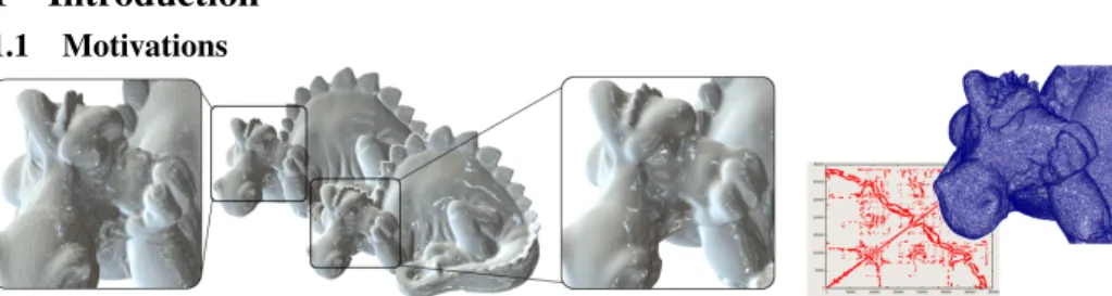
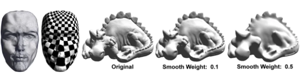
Fig. 1. Our CNC applied to mesh smoothing. Left: initial mesh; Center: smoothed mesh; Right: geometry processing with irregular meshes yield matrices with arbitrary non-zero patterns. There-fore, classic GPGPU techniques cannot be used. Our CNC implements a general solver on the GPU that can process these irregular matrices
In the last few years, graphics processors have evolved from rendering simple 2D objects to rendering real-time realistic 3D environments. Their raw power and memory bandwidth have grown so quickly that they significantly overwhelm CPU specifications. For instance, a 2GHz CPU has a theoretical peak performance of 8 GFlops (4 floating point operations per cycle using SSE), whereas modern GPUs have an observed peak performance of 350 GFlops [1].
Moreover, graphics card manufacturers have recently introduced new APIs ded-icated to general purpose computations on graphics processor units (GPGPU [2]):
CUDA from NVIDIA [3] and CTM from ATI [4]. These APIs provide low-level or direct access to GPUs, exposing them as large arrays of parallel processors.
Numerical solvers play a central role in many optimization problems that can be strongly accelerated by using GPUs. The key point is parallelizing these algorithms in a way that fits the highly parallel architecture of modern GPUs. As shown in Figure 1, our GPU-based Concurrent Number Cruncher (CNC) accelerates optimization algorithms and Partial Differential Equations (PDE)s solvers. Our CNC can solve large irregular problems, based on a very general sparse storage format of matrices, and is designed to exploit the computational capabilities of GPUs to their full extent.
As an example, we demonstrate our solver on two different geometry processing algorithms, namely LSCM [5] (mesh parameterization) and DSI [6] (mesh smoothing). As a front-end to our solver, we use the general OpenNL API [7].
In this work, we focus on iterative methods since they are easier to parallelize and have a smaller memory footprint than direct solvers, they can be applied to very large sparse matrices, and only a few iterations are needed in interactive contexts. Hence, our CNC efficiently implements on the GPU using the CTM API a Jacobi-preconditioned conjugate gradient solver [8] with a Block Compressed Row Storage (BCRS) of sparse matrices (section 1.2 and 2.1). The BCRS format is much more efficient than the simple Compressed Row Storage format (CRS) by enabling register blocking strategies, which reduce the required memory bandwidth [9].
Moreover, we compare our GPU-CTM implementation of vector operations with the CPU ones from the Intel Math Kernel Library (MKL) [10] and the AMD Core Math Library (ACML) [11], which are highly multithreaded and SSE3 optimized. For sparse matrix operations, we compare our GPU implementation with our SSE2 optimized CPU one since neither the MKL nor the ACML handle the BCRS format. Note that the CUDA BLAS library (CuBLAS) does not provide sparse matrix storage structures. 1.2 The Preconditioned Conjugate Gradient Algorithm
The preconditioned Conjugate Gradient algorithm is a well known method to itera-tively solve a symmetric definite positive linear system [8] (extensions exist for non-symmetric systems, see [12]). As it is iterative, it can be used to solve very large sparse linear systems where direct solvers cannot be used due to their memory consumption.
Given the inputs A, b, a starting value x, a preconditioner M, a maximum number of iterations imaxand an error tolerance ε < 1, the linear system expressed as Ax = b can
be solved using the preconditioned conjugate gradient algorithm described as follows:
i← 0; r ← b − Ax; d ← M−1r;
δnew← rTd; δ0← δnew;
while i < imaxand δnew> ε2δ0do
q ← Ad; α ←δnew dTq; x ← x + αd; r ← r − αq; s ← M−1r; δ old← δnew; δnew← rTs; β ←δδnew old; d ← r + βd; i ← i + 1; end
In this paper, we present an efficient implementation of this algorithm using the Jacobi-preconditioner (M = diag(A)) for large sparse linear systems using hardware acceleration through the CTM-API [4].
1.3 Previous Works on GPU Solvers
Depending on the discretization of the problem, solving PDEs involves band, dense or general sparse matrices. Naturally, the different types of matrices lead to specific solver implementations. Most of these methods rely on low-level BLAS APIs.
Band matrices
The first type of solver developed on GPUs were band solvers [13]. This is due to the natural and efficient mapping of band matrices into 2D textures. Most of the work done in this field was for solving the pressure-Poisson equation for incompressible fluid flow simulation applied to textures.
Dense matrices
Direct solvers for dense matrices were also implemented on GPUs for a Cholesky de-composition [14], and for both Gauss-Jordan elimination and LU dede-composition [15]. General sparse matrices
PDEs discretized on irregular meshes leads to solve irregular problems, hence call for a general representation for sparse matrices. Two authors showed the feasibility of im-plementing the Compressed Row Storage format (CRS). Bolz et al. [16] use textures to store non-zero coefficients of a matrix and its associated two-level lookup table. The lookup table is used to address the data and to sort the rows of the matrix according to the number of non-zero coefficients in each row. Then, an iteration is performed on the GPU simultaneously over all rows of the same size to complete, for example, a matrix-vector product operation. Another approach was proposed by Krüger and West-erman [13], based on vertex buffers (one vertex is used for each non-zero element). Our CNC method also implements general sparse matrices on the GPU, but uses a more compact representation of sparse matrices, and replaces the CRS format with BCRS (Block Compressed Row Storage) [9] to optimize cache usage and enable regis-ter blocking and vector computations.
New APIs, New Possibilities
Previous works on GPGPU used APIs such as DirectX [17] or OpenGL 2.0 [18] to ac-cess GPUs and use high-level shading languages such as Brook [19], Sh [20] or Cg [21] to implement operations. Using such graphics-centric programming model devoted to real-time graphics limits the flexibility, the performance, and the possibilities of modern GPUs in terms of GPGPU.
Both ATI [4] and NVIDIA [3] recently announced or released new APIs, respec-tively CTM and CUDA, designed for GPGPU. They provide policy-free, low-level hardware access, and direct access to the high-bandwidth latency-masking graphics memory. These new drivers hide useless graphical functionalities to reduce overheads and simplify GPU programming. In addition to our improved data structures, we use the CTM API to improve performance.
1.4 Contributions
The Concurrent Number Cruncher is a high-performance preconditioned conjugate gra-dient solver on the GPU using the new ATI-CTM API dedicated to GPGPU which re-duces overheads and provides fine controls for optimizations. The CNC is based on a general optimized implementation of sparse matrices using BCRS blocking strategies, and optimized BLAS operations through massive parallelization and vectorization of the processing. To our knowledge, this is the first linear solver on the GPU that can be efficiently applied to unstructured optimization problems.
2
The Concurrent Number Cruncher (CNC)
The CNC is based on two components: an OpenGL-like API to iteratively construct a linear system (OpenNL [7]) and a highly efficient implementation of BLAS functions. The following sections present some usual structures in supercomputing used in the CNC, how we optimized them for modern GPUs and important implementation fea-tures, which proved critical for efficiency.
2.1 Usual Data Structures in Supercomputing Compressed Row Storage (CRS)
Compressed row storage [9] is an efficient method to represent general sparse matrices (Figure 2). It makes no assumptions about the matrix sparsity and stores only non-zero elements in a 1D-array, row by row. It uses an indirect addressing based on two lookup-tables to retrieve the data: (1) a row pointer table used to determine the storage bounds of each row of the matrix in the array of non-zero coefficients, and (2) a column index table used to determine in which column the coefficient lies.
The Sparse Matrix-Vector Product Routine (SpMV)
The implementation of a conjugate gradient involves a sparse matrix-vector product (SpMV) that takes most of the solving time [12]. This product y ← Ax is expressed as:
for i = 1 to n, y[i] =
∑
j
ai, jxj
Since this equation traverses all rows of the matrix sequentially, it can be implemented efficiently by exploiting, for example, the CRS format (code for a matrix of size n × n):
for i = 0 to n − 1 do y[i] ← 0
for j = row_pointer[i] to row_pointer[i + 1] − 1 do y[i] ← y[i] + values[ j] × x[column_index[ j]] end
end
The number of operations involved during a sparse product is two times the number of non-zero elements of A [12]. Compared to a dense product that takes 2n2operations, the CRS format significantly reduces processing time.
2.2 Optimizing for the GPU
The massively parallel Single Instruction/Multiple Data (SIMD) architecture of modern GPUs calls for specific optimization and implementation of algorithms. GPUs offer two main levels of parallelism through multiple pipelines and vector processing, and several possibilities of optimizations presented in this subsection.
Multiple Pipelines
Multiple pipelines can be used to process data with parallelizable algorithms. In our implementation, each element of y is computed by a separate thread when computing the y ← Ax sparse operation (SpMV). This way, each thread iterates through a row of elements of the sparse matrix A to compute the product.
To maximize performance and hide memory-latencies, the number of threads used must be higher than the number of pipelines. For example, on an NVIDIA G80 that has 128 pipelines, y size should be an order of magnitude higher than 128 elements.
Similarly, operations on vectors, as the SAXPY computing the equation y←α×x+y, are parallelized by computing a unique element of the result y per thread.
To parallelize the vector dot product operation, the CNC implements an iterative sum-reduction of the data as in [13]: at each iteration, each thread reads and processes 4 scalars and writes one resulting scalar. The original n-dimensional vector is hence reduced by 4 at each iteration until only one scalar remains, after log4(n) iterations. Vector Processing
Some GPU architectures (e.g. ATI X1k series) process the data inside 4-element vector-processors. For such architectures, it is essential to vectorize the data inside 4-element vectors to maximize efficiency. Since our implementation targets a vector GPU archi-tecture (ATI X1k series), all operations are vectorized. On a scalar archiarchi-tecture like the NVIDIA G80, data do not need to be vectorized. However, for random memory ac-cesses, it is better to read one float4 than four float1 since the G80 architecture is able to read 128bits in one cycle and one instruction. Note that on a CPU it is possible to use SSE instructions to vectorize data processing.
Register Blocking: Block Compressed Row Storage (BCRS)
Unlike previous approaches which investigate, at best, only CRS format [13, 16], our CNC uses an efficient GPU implementation of the BCRS format. Note that, even on the CPU, BCRS is faster than CRS [9]. The BCRS groups non-zero coefficients in blocks of size BN × BM to use the maximum memory fetch bandwidth of GPUs, take advantage of registers to avoid redundant fetches, and reduce the number of indirections thanks to the reduced size of the lookup tables.
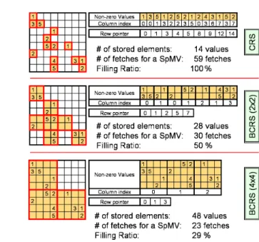
When computing a product of a block spanned over more than one row, it is possible to read only once the associated values from x of the block, store these values in regis-ters, and reuse them for each row of the block, saving several texture-fetches. Figure 2 illustrates the influence of the block size on the number of fetches. For 4-component vector architectures, fetching and writing scalars 4 by 4 maximizes both read and write bandwidth. It is therefore useful to process all four elements of y at the same time, and use blocks of size 4x4. Once the double indirection to locate a block using the lookup-tables is solved, 4 fetches are required to read a 4x4 block, 1 to read the corresponding
Fig. 2. Compressed Row Storage (CRS) and Block Compressed Row Storage (BCRS) examples for the same matrix. The number of stored elements counts all stored elements, useful or not. The number of fetches required to achieve a sparse matrix-vector product (SpMV) is provided for a 4-vector architecture, less fetches being better for memory bandwidth. The filling ratio indicates the average rate of non-zero data in each block, higher filling ratio being better for the computations
4-scalars of x, and 1 write to output the 4-scalars of the product result into y. Values of x are stored in registers, and reused for each row of the block, which results in fewer fetches than in a classical CRS implementation.
The reduced sizes of the lookup tables reduce memory requirements and, more im-portantly, the number of indirections to be solved during a matrix operation (each indi-rection results in dependent memory fetches, which introduces memory latencies).
Although a large block size is optimal for register and bandwidth usage, it is adapted only to compact matrices to avoid sparse blocks (Figure 2). The CNC implements 4x4 blocks, and also 2x2 blocks to handle cases where the 4x4 blocks present a very low fill-ing ratio. In the SpMV operation for a vector architecture, this 2x2 block size is optimal regarding memory read of the coefficients of the block, but not to read the correspond-ing x values and to write the resultcorrespond-ing y values since only two scalars are read from x and written in y.
2.3 Technicalities
The CTM (Close-To-Metal) device is a dedicated driver for ATI X1k graphics cards [4]. It provides low-level access to both graphics memory and graphics parallel processors. The memory is exposed through pointers at the base addresses of the PCI-Express-memory (accessible from both the CPU and GPU), and of the GPU-PCI-Express-memory (only accessible from the GPU). The CTM does not provide any allocation mechanism, and lets the application fully manage memory. The CTM provides functions to compile and
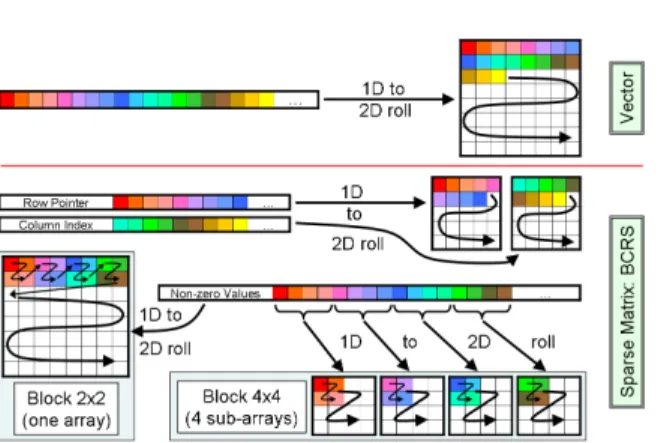
Fig. 3. Vector and BCRS sparse matrix storage representations on the GPU
load user assembly codes on the multiprocessors and functions to bind memory pointers indifferently to inputs or outputs of the multiprocessors.
Our CNC implements a high-level layer for the CTM hiding memory management by providing dynamic memory allocation for both GPU and PCI-Express RAM.
As shown in Figure 3, the CNC rolls vectors into 2D memory space to benefit from the 2D memory-cache of GPUs, and hence can store very large vectors in one chunk (on an ATI-X1k, the maximum size of a 2D array of 4-component vectors is 40962). The
BCRS matrix format uses three tables to store the column indices, the row pointers and the non-zero elements of the sparse matrix. The row pointer and column index tables are rolled as simple vectors, and the non-zero values of the matrix are rolled up depending on the block size of the BCRS format. Particularly, the CNC uses strip mining strategies to efficiently implement various BCRS formats. For the 2x2 block size, data are rolled block by block on one 2D-array. For the 4x4 block size, data are distributed into 4 sub-arrays fulfilled alternatively with 2x2 sub-blocks of the original 4x4 block as in [22]. Retrieving the 16 values of a block can be achieved by four memory fetches from the four sub-arrays at exactly the same 2D index, maximizing the memory fetch capabilities of modern GPUs and limiting address translation computations.
The CNC provides a high-level C++ interface to create and manipulate vectors and matrices on the GPU. Vector or matrix data is automatically uploaded to the GPU mem-ory at their instantiation for later use in BLAS operations. The CNC also pre-compiles and pre-allocates all assembly codes to optimize their execution. To execute a BLAS operation, the CNC binds the inputs and outputs of data on the GPU and calls the cor-responding piece of assembly code.
The assembly code performing a BLAS operation is made of very “Close-To-Metal" vector instructions as multiply-and-add or 2D memory fetch. It is finely tweaked using semaphore instructions to asynchronously retrieve data, helping in a better paralleliza-tion/masking of the latencies. The assembly code implementing a sparse matrix-vector product counts about a hundred lines of instructions, and uses about thirty registers. The number of used registers closely impacts performance, so we minimized their use.
The SpMV routine executes a loop for each row of blocks of a sparse matrix that can be partially-unrolled to process blocks by pair. This allows to asynchronously pre-load
data and better mask the latencies of the graphics memory, especially for consecutive dependent memory lookups. We increase the SpMV performance of about 30% by pro-cessing blocks two by two for both 2x2 and 4x4 block sizes.
As the GPU memory is managed by pointers, outputs of an assembly code can be bound to inputs of the next one, avoiding large overheads or useless data copy. In the conjugate gradient algorithm, the CPU program only calls the execution of assembly codes on the GPU in order, and binds/switches the inputs and outputs pointers. At the end of each iteration, the CPU retrieves only one scalar value (δ) to decide to exit the loop if necessary. Finally, the result vector is copied back to the PCI-Express memory accessible to both the GPU and the CPU. Hence, the whole main loop of the conjugate gradient is fully performed on the GPU.
3
Performance
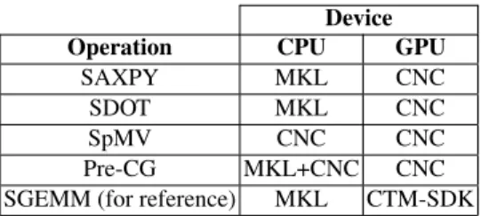
The preconditioned conjugate gradient algorithm for sparse matrices requires BLAS primitives for which this section provides comparisons in GFlops and percentage of efficiency for CPU and GPU implementations in the CNC. See Table 1 to get the list of implementations used for each operation on each hardware device.
For the SAXPY and SDOT benchmarks on the CPU, we used the Intel Math Kernel Library (MKL) [10] and the AMD Core Math Library (ACML) [11] which are highly multithreaded and optimized using SSE3 instructions. The CPU performance was, on average, close between the MKL and the ACML, hence we choose to only present the results from the former. The SpMV benchmark on the CPU is based on our multi-threaded SSE2 optimized implementation, since both the MKL and the ACML do not support the BCRS format.
Device Operation CPU GPU
SAXPY MKL CNC
SDOT MKL CNC
SpMV CNC CNC
Pre-CG MKL+CNC CNC SGEMM (for reference) MKL CTM-SDK
Table 1. Implementations used according to the operation and computing device: CNC is our, MKL is the Intel one, and CTM-SDK the ATI one
To be absolutely fair, GPU results take into account all overheads introduced by the graphics cards (cf. section 3.4). All benchmarks were performed on a dual-core AMD Athlon 64 X2 4800+, with 2GB of RAM and an AMD-ATI X1900XTX with 512MB of graphics memory.
Benchmarks were performed at least 500 times to average the results, use synthetic vectors for the SAXPY and SDOT cases, synthetic matrices for the SGEMM case (given for reference), and real matrices built from the set of meshes described in Table 2 for other cases. Figure 4 shows parameterization and smoothing examples of respectively the Girl Face 3 and Phlegmatic Dragon models, both computed using our CNC on the GPU.
Fig. 4. Parameterization of the Girl Face 3 and smoothing of the Phlegmatic Dragon using our CNC solver on the GPU
Parameterization Smoothing Mesh #var #non-zero #var #non-zero Girl Face 1 1.5K 50.8K 2.3K 52.9K Girl Face 2 6.5K 246.7K 9.8K 290.5K Girl Face 3 25.9K 1.0M 38.8K 1.6M Girl Face 4 103.1K 4.2M 154.7K 6.3M Phlegmatic Dragon 671.4K 19.5M 1.0M 19.6M
Table 2. Meshes used for testing matrix operations. This table provides: the number of unknown variables computed in case of a parameterization or a smoothing of a mesh, denoted by #var, and the number of non-zero elements in the associated sparse-matrix denoted by #non-zero (data courtesy of Eurographics for the Phlegmatic Dragon)
3.1 BLAS Vector Benchmarks
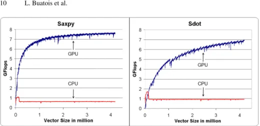
Figure 5 presents benchmarks of SAXPY (y ← α × x + y) and SDOT/sum-reduction operations on both CPU and GPU respectively using the MKL and our CNC. While the performance curve of the CPU stays steady, the GPU performance increases with the vector size. Increasing the size of vectors, hence the number of threads, helps the GPU in masking the latencies when accessing the graphics memory. For the SDOT, performances increase not as fast as for the SAXPY due to its iterative computation that introduces more overheads and potentially more latencies which need to be hidden. At best, our GPU implementation is 12.2 times faster than the CPU implementation of the MKL for the SAXPY and 7.4 times faster for the SDOT.
3.2 SpMV Benchmarks
Testing operations on sparse-matrices is not straightforward since the number and lay-out of non-zero coefficients strongly govern performance. To test sparse matrix-vector product (SpMV) operations and preconditioned conjugate gradient, we choose five models and two tasks (parameterization and smoothing) which best reflect typical situ-ations in geometry processing (Figure 4 and Table 2).
Figure 6 shows the speed of the SpMV for various implementations and applica-tions. Four things can be noticed: (1) CPU performance stays relatively stable for both problems while the GPU performance increases according to the increasing size of the matrices, (2) thanks to register blocking and vectorization, BCRS 4x4 is faster than 2x2 (which is also faster than CRS) for CPUs and GPUs, (3) GPU is about 3.1 times faster than CPU with SSE2 for significant mesh sizes, and (4) multithreaded-SSE2 implemen-tation enabling vector processing on the CPU is about 2.5 times faster than standard
Fig. 5. SAXPY (y ← α × x + y) and SDOT (sum-reduction of a vector) performances comparison in function of the processed vector size between the CPU MKL implementation and our GPU implementation
implementation. For very small matrices, the CNC just compares to CPU implementa-tions, but, in that case, a direct solver would be more appropriate.
3.3 Preconditioned Conjugate Gradient Benchmarks
Performance of the main loop of a Jacobi-preconditioned conjugate gradient is provided in Figure 6. Since most of the solving time, about 80%, is spent within the SpMV whatever hardware device is used, the SpMV governs the solver performance, and the comments for the SpMV are also applicable here. GPU solver runs 3.2 times faster than the CPU-SSE2, and CPU-SSE2 solver runs 1.8 times faster than the non-SSE2. As for the SpMV routine, the CNC is inefficient for very small matrices where direct solvers are anyway better.
3.4 Overheads and Efficiency
Overheads introduced when copying, binding, retrieving data or executing shader pro-grams on the GPU were the strong bottlenecks of all previous works. New GPGPU APIs like CTM or CUDA can increase performance if well used (cf. section 2.3). Dur-ing our tests, the total time spent for the processDur-ing on the GPU was always higher than 93%, meaning that less than 7% percents were for the overheads, showing a great improvement as compared to previous works.
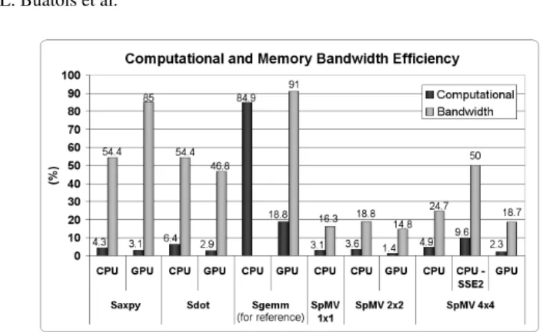
CPU and GPU architectures are bound by their maximum computational perfor-mance and maximum memory bandwidth. Their efficiency mainly depends on the im-plemented operations (Figure 7). For example, low computation operations like the SAXPY or the SDOT are limited by the memory bandwidth, and not by the theoret-ical computational peak power. The SAXPY achieves high bandwidth efficiency on GPUs, near 91%, but very low computational efficiency, near 3.1%. Conversely, for reference, a dense matrix-matrix product (SGEMM) on the GPU can achieve a good computational efficiency, near 18.75%, and a very good memory bandwidth efficiency, near 91% (used SGEMM implementation comes from the ATI CTM-SDK). In the case of SpMV operations, both computational and memory bandwidth efficiency are low on GPUs and CPUs (although SSE2 greatly helps). This is due to the BCRS format that
Fig. 6. Performance comparison of the SpMV (sparse matrix-vector product) and the Jacobi-Preconditioned Conjugate Gradient Main Loop between CPU standard, CPU multithreaded-SSE2 optimized, and GPU implementations in case of computing a mesh parameterization or smooth-ing for CRS (no blocksmooth-ing), BCRS 2x2 and BCRS 4x4
implies strong cache-miss and several dependent memory fetches. Nevertheless, as pre-viously written, our CNC on the GPU performs the SpMV 3 times faster than on the CPU.
4
Conclusions
The Concurrent Number Cruncher aims at providing the fastest possible sparse linear solver through hardware acceleration using new APIs dedicated to GPGPU. It uses blockcompressed row storage, which is faster and more compact than compressed row storage, enabling register blocking and vector processing on GPUs and CPUs (through SSE2 instructions). To our knowledge, this makes our CNC the first implementation of a general symmetric sparse solver that can be efficiently applied to unstructured optimization problems.
Our BLAS operations on the GPU are 12.2 and 8 times faster for respectively SAXPY and SDOT operations than on the CPU using SSE3-optimized Intel MKL li-brary. As compared to our CPU SSE2 implementation, the SpMV is 3.1 times faster, and the Jacobi-preconditioned conjugate gradient 3.2 times. We show that on any de-vice BCRS-4x4 is significantly faster than 2x2, and 2x2 significantly faster than CRS. Note that our benchmarks include all overheads introduced by the computations on the GPU.
Fig. 7. Percentage of computational and memory bandwidth efficiency of different operations implemented on the CPU and the GPU for 10242 vector size, 10242 dense matrix size and Girl Face 4 model to test the SpMV in case of a parameterization. See Table 1 to determine used implementations
While the GPGPU community is waiting for GPU double floating point precision, graphics cards only provide single precision for the moment. Hence, our CNC targets applications that do not require very fine accuracy but very fast performance.
As previously shown, operations on any device are limited either by the memory bandwidth (and its latency), or by the computational power. In most BLAS operations, the limiting factor is the memory bandwidth, which was limited to 49.6 GB/s for our tested GPU. According to ATI announces, the memory of their next graphics card -the high-end R600- will handle between 110 to 140 GB/s, which will surely strongly increase the performance of our CNC and the gap with CPU implementations.
We plan to extend the parallelization of the CNC across multi-GPUs within a PC (based on SLI or CrossFire configurations), across PC clusters, or within new visual computing systems like the NVIDIA Quadro Plex containing multiple graphics cards with multiple GPUs inside one dedicated box. Thus, we will use the CUDA API from NVIDIA in the CNC to be compatible with the largest possible panel of GPUs. We will build and release a general framework for solving sparse linear systems, including full BLAS operations on sparse matrices and vectors, accelerated indifferently by an NVIDIA with CUDA, or by an ATI with CTM. Note also that iterative non-symmetric solvers (Bi-CGSTAB and GMRES) can be easily implemented using our framework. We will experiment them in future works.
5
Acknowledgements
The authors thank the members of the GOCAD research consortium for their support (www.gocad.org), Xavier Cavin, and Bruno Stefanizzi from ATI for providing the CTM API and the associated graphics card.
References
1. Buck, I., Fatahalian, K., Hanrahan, P.: Gpubench: Evaluating gpu performance for numerical and scientific applications. In: Proceedings of the 2004 ACM Workshop on General-Purpose Computing on Graphics Processors. (2004)
2. : GPGPU (General-Purpose computation on GPUs). www.gpgpu.org
3. Keane, A.: CUDA (compute unified device architecture). In: http://developer.nvidia.com/object/cuda.html. (2006)
4. Peercy, M., Segal, M., Gerstmann, D.: A performance-oriented data-parallel virtual machine for gpus. In: ACM SIGGRAPH’06. (2006)
5. Levy, B., Petitjean, S., Ray, N., Maillot, J.: Least squares conformal maps for automatic texture atlas generation. In ACM, ed.: SIGGRAPH 02, San-Antonio, Texas, USA. (2002) 6. Mallet, J.: Discrete Smooth Interpolation. Computer Aided Design 24(4) (1992) 263–270 7. Levy, B.: Numerical methods for digital geometry processing. In: Israel Korea Bi-National
Conference. (November 2005)
8. Hestenes, M.R., Stiefel, E.: Methods of Conjugate Gradients for Solving Linear Systems. J. Research Nat. Bur. Standards 49 (1952) 409–436
9. Barrett, R., Berry, M., Chan, T.F., Demmel, J., Donato, J., Dongarra, J., Eijkhout, V., Pozo, R., Romine, C., der Vorst, H.V.: Templates for the Solution of Linear Systems: Building Blocks for Iterative Methods, 2nd Edition. SIAM, Philadelphia, PA (1994)
10. Intel: Math kernel library. www.intel.com/software/products/mkl 11. AMD: Amd core math library. http://developer.amd.com/acml.jsp
12. Shewchuk, J.R.: An introduction to the conjugate gradient method without the agonizing pain. Technical report, CMU School of Computer Science (1994) ftp://warp.cs.cmu.edu/quake-papers/painless-conjugate-gradient.ps.
13. Krüger, J., Westermann, R.: Linear algebra operators for gpu implementation of numerical algorithms. ACM Transactions on Graphics (TOG) 22(3) (2003) 908–916
14. Jung, J.H., O’Leary, D.P.: Cholesky decomposition and linear programming on a gpu, Schol-arly Paper, University of Maryland (2006)
15. Galoppo, N., Govindaraju, N.K., Henson, M., Manocha, D.: LU-GPU: Efficient algorithms for solving dense linear systems on graphics hardware. In: SC ’05: Proceedings of the 2005 ACM/IEEE conference on Supercomputing, Washington, DC, USA, IEEE Computer Society (2005) 3
16. Bolz, J., Farmer, I., Grinspun, E., Schröder, P.: Sparse matrix solvers on the GPU: conjugate gradients and multigrid. ACM Trans. Graph. 22(3) (July 2003) 917–924
17. Microsoft: Direct3d reference. msdn.microsoft.com (2006)
18. Segal, M., Akeley, K.: The OpenGL graphics system: A specification, version 2.0. www.opengl.org (2004)
19. Buck, I., Foley, T., Horn, D., Sugerman, J., Fatahalian, K., Houston, M., Hanrahan, P.: Brook for gpus: stream computing on graphics hardware. ACM Trans. Graph. 23(3) (2004) 777– 786
20. McCool, M., DuToit, S.: Metaprogramming GPUs with Sh. AK Peters (2004)
21. Fernando, R., Kilgard, M.J.: The Cg Tutorial: The Definitive Guide to Programmable Real-Time Graphics. Addison-Wesley Longman Publishing Co., Inc., Boston, MA, USA (2003) 22. Fatahalian, K., Sugerman, J., Hanrahan, P.: Understanding the efficiency of gpu
algo-rithms for matrix-matrix multiplication. In: HWWS ’04: Proceedings of the ACM SIG-GRAPH/EUROGRAPHICS conference on Graphics hardware, New York, NY, USA, ACM Press (2004) 133–137