A computational model for the isothermal assembly of tiled DNA nanostructures

A Computational Model for the Isothermal Assembly of Tiled DNA Nanostructures

by

Benjamin Steele

B.S., Biology

California Institute of Technology, 2010

Submitted to the Department of Biology

in Partial Fulfillment of the Requirements for the Degree of

Master of Science in Biology

at the

MASSACHUSETTS INSTITUTE OF TECHNOLOGY

,NASSCHSETS uI4STrJE

CFTECHNOLOGY

IBRARIES

February 2014

0 2014 Massachusetts Institute of Technology. All rights reserved.

Signature of A uthor ... . ...

Department of Biology

January 31, 2014

Certified by ...

Mark Bathe Assistant Professor of Biological Engineering

Thesis Supervisor

Accepted by...

/

Associate Professor of Biology Chair, Department of Biology Graduate Committee

A Computational Model for the Isothermal Assembly of Tiled DNA Nanostructures

by

Benjamin Steele

B.S., Biology

California Institute of Technology, 2010

Submitted to the Department of Biology

on January 31, 2014 in Partial Fulfillment

of the Requirements for the Degree of

Master of Science in Biology

ABSTRACT

Complex DNA nanostructures have proven difficult to assemble from starting materials.

Inefficient nanostructure assembly constitutes a barrier to the widespread use of DNA

nanotechnology and is difficult to investigate experimentally due to the complicated nature of the

assembly. This work introduces a type of tile assembly model, the isothermal tile assembly

model (iTAM). The iTAM seeks to capture the behavior of assembling DNA tile nanostructures

to identify design factors and reaction conditions which improve assembly yields.

Simulations using the iTAM model explain the experimental observation that only a

narrow range of temperatures permit optimal isothermal assembly of tile-based DNA

nanostructures. This narrow temperature range reflects a balance between the stabilization of

non-designed interactions at low temperatures and the destabilization of the overall designed

structure at high temperature. Simulations based on the iTAM are effective at estimating the

temperature of optimal assembly unique to 25 two-dimensional tile designs, with an mean error

of estimation of 4.6 degrees C.

Results from the iTAM indicate that optimal assembly temperatures are determined

largely by the strength of tile-tile domain interactions. For a given tile design, tile concentration

and the length of time represent convenient axes of control over tile assembly. Kinetic trapping

that blocks complete assembly of a tile design is likely to be overcome by increasing the both

temperature and tile concentration in the assembly reaction. Such a change also substantially

decreases the computationally predicted time required for complete assembly.

Thesis Supervisor: Mark Bathe

Acknowledgements

Thanks are due to Mark Bathe and Amy Keating for their guidance during my studies; to Cameron Myhrvold and Peng Yin, whose enthusiasm for DNA engineering was infectious; and to all the members of the Laboratory for Computational Biology and Biophysics (especially Matthew Adendorff, Aprotim Mazumder, and Keyao Pan).

2

3

1. Introduction to DNA Nanotechnology and Self-Assembly 5

1.1 Basics of DNA Nanostructures... 5

1.2 DNA Nanostructures: Applications... 8

1.3 Assembly of DNA Nanostructures... 11

2. Models for DNA Tiling Self-Assembly 14 2.1 The Abstract Tile Assembly Model... 14

2.2 The Kinetic Tile Assembly Model... 17

2.3 The Isothermal Tile Assembly Model... 20

2.4 The Thermodynamics of Self-Assembly... 21

3.

The

3.1

3.2

3.3

3.4

3.6

3.7

Results from the SST System ... 27

Im plem entation of the iTAM ... 30

Simulation Results: Optimal Assembly Temperatures...34

N ucleation... 40

Tim e and Concentration... 43

Conclusions... 46 47 50

Contents

Chapter 1. Introduction to DNA Nanotechnology and Self-Assembly

1.1 Basics of DNA Nanostructures

DNA nanotechnology uses DNA as a building material to create structures and active

devices with nanoscale sizes. Though simple in concept, DNA nanotechnology has attracted interest from such disparate fields as biochemistry, computer science, and mechanical engineering, with a corresponding range of suggested applications.

DNA: information store and building material

DNA is a basic building block of life on Earth. Nature uses DNA to store and copy

information that encodes the basic macromolecules of the cell: DNA, RNA, and proteins. Though genome sizes and organization differ between organisms, the physical structure and basic patterns of DNA layout are shared between all known forms of life. DNA nanotechnology uses the same materials toward a different purpose. In DNA nanotechnology, the specific pairings and stable structure of DNA are used not for information storage but rather to create architectural patterns on the nanoscale.

DNA consists of a long strand of monomer units, or bases, that are joined together by

covalent bonds. Four different types of monomers are found in nature, each of which can form stable hydrogen bonds with only one of the other monomer species (adenine with thymine;

cytosine with guanine). Such base pair interactions underpin the form in which DNA is most commonly found: the familiar double helix, where two strands of DNA run parallel to each other

in opposite orientations and every base is hydrogen-bonded to its appropriate complement on the other strand. This form is further stabilized by the exclusion of water molecules from the core of the helix and especially by stacking effects between adjacent bases on the same strand.

One specific form of such interaction, called B-DNA, describes the substantial majority of all DNA found in natural and designed DNA applications. B-DNA is characterized by a rise per base pair (bp) along the helix of 0.332 nm, with 10.5 bp constituting a full turn of the helix. This double-helical structure is stable against thermal dissociation if the strands are at least 15 bp

2.0 nm

long [1]. Two helical grooves run along the exterior

of the double helix. The larger of these grooves, the

C

major groove, is frequently used as a binding site

A T

for protein complexes that copy DNA or regulate

gene activity.

10.5 bp

DNA nanotechnology is feasible because the

(3.5

nm)

interaction of two strands of DNA is in general

both readily predictable and highly programmable.

Under appropriate assembly conditions, two

(0.33 nm)

strands will specifically and stably bind only if

they share a long stretch of complementary

Figure 1: B-DNA. The view is

nucleotides. The resulting strand-strand binding

perpendicular to the helical axis, and

the first three base pairs are labeled.

region is typically a simple double helix that can be

modeled as a stiff rod over lengths of around 10 nm

[1]. Complex structures can be built by introducing breaks between double-stranded rods, either

by placing a nick in which the backbone of one strand is discontinuous between successive base

pairs or by placing a region of single-stranded DNA between double-stranded segments. Such

breaks introduce flexibility into the structure and permit the design of bends [2].

The simple design properties of DNA nanostructures contrast with those for designed

protein-protein or protein-ligand interactions, where tertiary structure and interactions are more

variable. Compared to inorganic nanostructures produced through methods like

photolithography, DNA allows the formation of structures at smaller scales, can be made to

undergo conformational changes, and exhibits optimal function only in a biological environment.

This last is a significant hinderance to DNA nanotechnology's widespread utilization: DNA

nanostructures require an aqueous environment and are frequently intolerant of significant

changes in environmental temperature or salinity.

DNA nanotechnology

The first suggestion that DNA could be used as a building material for nanotechnology dates to Nadrian Seeman in 1982 [3,4]. Seeman suggested that a three-dimensional cubic DNA lattice could be used to fix the position of covalently-bound particles difficult to crystallize, conferring a ordered pattern that could be used for X-ray structure determination of the bound particles. In practice it is difficult to build a structure from DNA with sufficient size and rigidity for this purpose, though recently a DNA-based liquid crystal has been successfully used to orient membrane proteins for NMR structure determination [5,6].

More fruitful was the basic concept that synthetic DNA strands with designed regions of base pairing can self-assemble into nanostructures. In 1991 Seeman's lab succeeded in producing a cube, sparking significant interest in DNA nanotechnology. Work along similar lines has produced other polyhedra, such as tetrahedra and octahedra [7,8].

The desire to produce design patterns with broader application led Seeman and others to utilize a tiling pattern to generate larger structures from simpler components, a strategy described

in greater detail below. The earliest designs used DNA tiles made rigid through the inclusion of

multiple crossovers to generate two-dimensional planar structures, which were later shown to be generalizable into hollow tubular forms [9,10]. Though successful, the tendencies toward large-scale disorder, the relative unsuitability for three-dimensional applications, and the low yields of complex structures have constrained the use of tile-based designs in favor of DNA origami, discussed below, in many settings. Recent work addresses some of these drawbacks, using single-stranded tiles (with fewer synthesized bases) to generate arbitrary 3D shapes on a grid pattern [11,12].

The introduction of DNA origami by Paul Rothemund in 2006 greatly enhanced the design, assembly, and yields of DNA nanostructures. In DNA origami designs, a single-stranded

DNA virus genome called the scaffold strand is folded up using small synthetic staple strands

that bind to multiple regions of the scaffold [13]. While the necessary inclusion of the large scaffold strand places constraints on the size, sequence, and layout of the DNA nanostructure design, DNA origami designs have been used to great success in a wide range of applications.

1.2 DNA Nanostructures: Applications

Engineering applications

Proposed engineering applications for DNA nanostructures have focused on the precise positioning and controllable nature of designed base pairing patterns. In one approach, DNA

nanostructures are used as a foundation to orient linked proteins and functional groups. Such

demonstrated designs include "printing" an array of DNA-linked gold nanoparticles onto a surface and constructing an efficient light-harvesting antenna by positioning dyes onto a DNA

cylinder [14,15]. One recent design of particular interest created an artificial membrane channel permeable to ions and single-stranded DNA by positioning covalently linked cholesterol

molecules at the sides of a multihelix bundle made with DNA origami [16].

a.

_

b.

flllfff

C.

Eu...

Figure 2: Designed DNA nanostructures.

(a) Planar DNA origami designs (left column) and corresponding AFM images from [13]. Structures are 100 nm wide.

(b) A variety of 2D shapes assembled from single-stranded DNA tiles [12]. Each AFM image

shown is 150 nm x 150 nm.

(c) A DNA nanorobot that shifts from a closed barrel conformation (top left) to a open conformation (right), releasing a protein payload, when unlocked by an antigen "key" [17].

Alternatively, DNA can be used as an active, mobile element. Changes in DNA base

pairing have been used to drive conformational changes in a nanostructure, provide motive

Such conformational changes have been harnessed to produce "smart" drug delivery vehicles

that exhibit enhanced drug delivery and improved cytotoxicity [20].

Computational applications

Computation through nanostructure assembly was first demonstrated by Len Adelman in

1994 and represents a distinct area of interest in tiled DNA structures [21]. Any desired structure

or, equivalently, computation result, can be generated using an appropriately chosen set of tiles

and temperatures, given certain assumptions [22]. A tiling DNA computer implemented in this

fashion could be enormously parallel, utilizing

logic gates (while as of 2013

microprocessors feature >1010 transistors)'. No calculation approaching this size has been

attempted, though computation through tiling has been demonstrated for proof-of-principle

problems such as assembling an XOR logic gate from tiles, performing binary operations, and

constructing a Sierpenski triangle [23-26].

DNA tiling computation is constrained by the large size of the tile set needed to carry out

nontrivial problems, by the time and temperature dependence required for a calculation, and by

the significant error rate of tile addition, all of which have been the subject of theoretical and

experimental investigation. Since the number of strands needed to encode a calculation grows

exponentially with the size of the problem, scaling up DNA computing to address interesting

problems demands prohibitive numbers of DNA species in practice [27]. Error rates further limit

calculation size: an error rate of 0.1%, comparable to the best achieved, requires that structures

not exceed 50 tiles in size to ensure 95% confidence that no error has occurred [25]. Finally, tile

computations are inefficient: only the growing edge of a tiled structure actively performs

calculations, and when growth is complete it is difficult to read out the computation result or

reuse tiles for a different problem. These considerations mean that DNA tile computation cannot

practically solve problems intractable on existing computers.

I

Figure 3: A Sierpinski triangle grown from self-assembled planar DAO-E tiles, from [26].

The scale bar is 100 nm.

(a) An tile placement error rate of

5%

produces disorder visible at larger scales.

(b) Detail from (a), with misplaced tiles shown with red crosses.

(c) A structure with growth initiated by an error and terminated by 3 errors (crosses).

More significant for future applications are comparatively trivial calculations for which

DNA as a material is uniquely suited. Relevant uses could include assembling a patterned layout

as a template for a nanodevice or performing a computation within a biological environment. In

a proof of principle, nanodevices composed of DNA alone have been built which can perform

signal processing based on multiple simultaneous environmental inputs [28, 29].

Similar

networks could be used in vivo to determine the state of a cell or biological process and used to

trigger a response

-

for instance, a caged toxin could be released into a cell if a DNA-based logic

network determined that the cell exhibited high levels of cancer metabolites.

1.3 Assembly of DNA nanostructures

Nanostructure design and assembly

Though structures as small as Seeman's cube are simple to design by hand, complex structures do not possess a single obvious correct design. DNA designs are difficult to scale up in practice: more or longer strands are required, which increases the cost of reactants. Further, complex designs are frequently more sensitive to assembly conditions and exhibit poor yields of correctly formed structures. To simplify nanostructure layout and assembly, large DNA structures are today typically designed using either a tiling pattern or a DNA origami design.

In a DNA tiling design, a simple DNA architectural element is repeated throughout a design to form a larger tiled structure. A tile can be any shape that fills space - triangles, hexagons, aperiodic tilings, and patterns incorporating multiple shapes are all possible. Most designs to date have used a rectangular "pixel" or cubical "voxel" unit that assembles to form a grid pattern. Unlike DNA origami structures, tiled structures are not constrained by the size of a scaffold strand: structures can be as small as a single tile and in theory have no maximum size. Tiled structures generally exhibit lower yields than comparably sized DNA origami structures: more strands must interact to form tiled structures, and errors in tiled structures can propagate throughout the structure because information on tile placement is derived only from local

interactions.

With a DNA origami design, a careful choice of folds produces any structure obtainable

by bending a wire or loop: barrels and planar folded patterns resembling an antiparallel B-pleated

sheet are common design motifs. In practice, DNA origami is a robust assembly method that

produces large structures with good yield and requires synthesized DNA only for the short staple

strands. A key concept for overall origami assembly, which contrasts with that for DNA tiles, is that the presence of the scaffold strand imposes a top-down organization that reduces large-scale disorder.

The assembly of a DNA nanostructure typically proceeds by placing all strands required into solution in a single reaction vessel, heating all strands to break any existing base pairs, and then gradually cooling the reaction in a slow thermal annealing ramp to room temperature.

Assembly requires the presence of salts, as DNA's negative electrostatic charge must be neutralized by cations for folding to occur. Small divalent cations (Mg2+) are especially effective

at stabilizing DNA nanostructures, since such cations can enter tightly packed structures to form coordination complexes with strands' negatively charged phosphate backbones.

Kinetic barriers affect DNA nanostructure assembly

Kinetic effects govern the assembly process of DNA nanostructures, as demonstrated by slow rates of folding and the observed hysteresis between folding and unfolding. The fully folded state is hugely favored at equilibrium (each 1 kcal/mol difference between states corresponds to a 5-fold factor at equilibrium), such that folded or nearly-folded states alone should be populated at equilibrium. This is not observed for large nanostructures, which instead exhibit low yields (10% yields are common) and a substantial degree of incomplete assembly

[30]. These effects can only be explained by the existence of a kinetic barrier to assembly that

prevents equilibrium occupation of the folded state.

DNA nanostructures exhibit substantial hysteresis between folding and unfolding, a

kinetic effect. Measured nanostructure folding temperatures are around 10 0C lower than unfolding temperatures [31, 32]. This requires one or both of the folding and unfolding processes to be out of equilibrium. Evidence points to the folding temperature being

time-dependent, indicating folding is subject to kinetic control [31]. Separate work has also

demonstrated that the folding rate of DNA origami is greatly enhanced at low temperatures in the presence of denaturant, as is expected if kinetic trapping governs folding rates [33].

Isothermal assembly

Recent work indicates DNA nanostructures' folding is subject to another kinetic effect: folding rates have substantial temperature dependence and are maximal below the structures' melting temperatures [31]. This phenomenon is well-known in polymer crystallization, and is explained by lower- and upper-temperature bounds to assembly (Tgiass and Tmelt, respectively) [34]. Tgiass is a kinetic barrier below which incorrect interactions that impede crystallization are stable over the time length studied. Tmeit is an equilibrium barrier, above which the ordered state

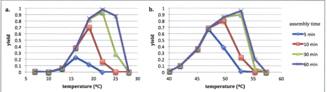
is unstable. Assembly rates are non-negligible only between Tgiass and Tmeit, and peak at an intermediate temperature Toptimal.

Several DNA nanostructure designs have been demonstrated to exhibit this peaked folding rate at a specific temperature, including both DNA origami and tiled DNA structures

[31,35]. When structure assembly is carried out isothermally at Toptimai, yields are greatly

enhanced relative to older protocols requiring a gradual temperature ramp and incubation times can be shortened from weeks to hours.

Understanding the nature of the kinetic barriers that block DNA nanostructure assembly and being able to set the temperature of optimum folding has the potential to greatly increase the yield, speed of folding, and range of environmental conditions under which DNA nanostructures are employed. This work seeks to do so by applying a model to analyze the assembly of a set of tiled DNA nanostructures that have been experimentally characterized.

Chapter 2. Models for DNA Tiling Self-Assembly

DNA nanostructure assembly occurs through a complex series of coupled reactions

between intermediates. Though nanostructure assembly is not understood in great detail, work over the course of two decades has produced models through which aspects of the assembly process can be analyzed. Such models are reduced models that rely on a number of simplifying assumptions about the nature of DNA assembly.

Sections 2.1 and 2.2 review two such models developed by Erik Winfree, the aTAM and

kTAM, and describe prior research into these models' properties. Section 2.3 provides motivation

for and outlines the iTAM, a variant of the kTAM developed for this work. The goal of the iTAM is to provide a model that can computationally recapitulate the isothermal assembly behavior experimentally observed in DNA tiles [35].

2.1 The Abstract Tile Assembly Model

The abstract tile assembly model (aTAM), introduced by Erik Winfree in 1998, extends the mathematical notion of Wang tiling to the problem of two-dimensional DNA nanostructure

assembly [22]. The aTAM takes as input the definition of a tile set, an initial "seed" structure,

and a "temperature" T, _{together termed the tile assembly system. Using these starting parameters,}

the aTAM then executes a Monte Carlo algorithm that simulates the irreversible growth of a tiled

structure. The following review of the aTAM is from Winfree, and is important to reproduce here

because the model's features and results underlie the kTAM and iTAM models discussed in sections 2.2 and 2.3 upon which this work is directly based [22].

Description

The tile set comprises n square tiles, or monomers, {ai, a2, ..., an}. Each tile in the tile set is defined by eight parameters: four edge labels {JON, aIE, ui,s, aiw} and four associated integer

1

I

2

U

if

0

1i

ifli

OkJ2

T =2

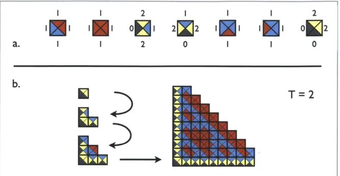
Figur 4: An example tileset for the abstract tile assembly model.

(a) An example tile set is shown. Different colors represent the four edge labels, and

numbers represent the edge strengths.

(b) Assembly of this tile system is shown at T

=

2. Under this condition assembly is

deterministic and produces a variant of the Sierpinski triangle (a portion shown at right).

For T = 0 or T

=

1 incorrect additions can occur and assembly does not yield a set pattern.

p(off)

koff = kf[e-'I+e

p(on)

=

on

kon+kof]

=7kf[mono.]

Figure 5: An example step in the

kTAM. A three-tile structure will lose

a tile at rate koff and gain a tile at rate

k0n. At left, possible structures after tile

dissociation. At right, the 7 possible sites for tile addition are shown with dashed outlines.

Tiles and binding strengths (units of

kBT) are as in Figure 4(a). The corner

tile is a fixed seed tile and cannot

dissociate.

a.

edges have identical labels and interact with strength 0 otherwise.

Structure assembly begins with a grid that is initially occupied by the input "seed"

structure. In each step of the simulation, as illustrated in Figure 4, a tile a is chosen at random

from the tile set and placed in a grid square that borders the existing structure. The new tile's

edge interaction strengths with the existing structure are scored and summed as

the new tile is retained and the structure grows in size by 1 tile. If Gnew

<

'r, the new tile is

removed and no growth occurs.

Per Winfree, any desired structure or computation result can be generated with an

appropriately chosen tile assembly system [22]. A tile assembly system may or may not be

deterministic, meaning it leads to a unique terminal assembly, and may or may not produce a

structure of finite size. Though unattractive for constructing physical nanostructures,

nondeterministic systems have been formally shown to possess greater computational power than

deterministic systems [36].

As described by Winfree, a typical tileset in the aTAM has tiles possessing edge

interaction strengths gi

=

1. This results in programmed structure growth that occurs at

2,

where a tile adds only if it attaches to correct partner tiles along two edges of the structure. (At

T =

1 a single correct edge match will yield tile addition.) If all edge labels are used only twice

in the final structure, a single correct edge match describes a unique position for the adding tile

and programmed growth will occur at

=

1. If edge labels are reused throughout the tileset, a

single edge match will not uniquely describe a position. Growth will then occur, but some errors

are stable and will be incorporated into the structure. At T= 0, all tile additions are stable and the

structure will grow indefinitely and without order; at

2, no additions are stable and growth

cannot occur. These bounds have been shown to be true only for rectangular tiles in two

dimensions: extension of the aTAM to three dimensions permits algorithmic tile assembly at

aTAMextensions

Numerous groups have sought to extend the aTAM by relaxing specific model

assumptions [38,39,40,4 1]. Of greatest relevance for the isothermal tile assembly model, outlined

in section 2.3, are extensions of the aTAM in which properties of the tiles are changed. Relaxing the constraint that tiles must be confined to interact in two dimensions leads to a model for flexible tiles which can efficiently encode certain graph-theoretic problems [40]. Models can be generated in which edges which do not share the same edge label nonetheless interact with nonzero strength [39]. The assumption that only monomer tiles are allowed to interact can be reduced through the staged assembly model, in which selected strands are assembled in separate reactions into subcomponents that are then mixed for final assembly [41], or the 2HAM model, where two structures assemble separately but at each step have a chance of merging [39]. Though of these only the edge-label constraint is relaxed in the isothermal tile assembly model, these extensions are significant in that they represent routes through which the assembly models discussed in Chapter 2 can be generalized to more complex tile systems and more realistic assembly conditions.

2.2 The Kinetic Tile Assembly Model

The kinetic tile assembly model (kTAM), introduced by Winfree concurrently with the aTAM, provides a more physically realistic description of DNA tile structure assembly than the aTAM [22]. In the kTAM, tile addition is considered to be a reversible chemical reaction. The properties and treatment of tile assembly of the kTAM have been previously described, but are key to this work and so are reviewed in the remainder of this section.

The kTAM takes as input a tile set, a seed structure, a physical temperature T, a tile concentration [monomer] = e-Gmc, and a kinetic rate constant kf. The edge strengths {gi o, ... , gi3} are now given in energy units (e.g. kcal/mol) and T is in Kelvin. Here, the ratio Gmc/gi is approximately equivalent to r as defined for the aTAM.

An assembly simulation with kTAM begins with the input "seed" structure. In each step, the m unfilled grid squares bordering the current structure are determined and placed in the set

U = {uJ, ... , um}. The h filled grid squares in the structure (the seed tile is excepted) have their interaction energies with other tile squares counted and summed, creating a set of h tile binding energies B = {b1, ..., bh}.

The tile monomer on-rate is assumed to be constant for each possible binding site. The

net on-rate is then given by:

kon = mkijmonomer]

The net off-rate is given by:

koff

The overall rate of events is ktot

=

k

n + koff. Using this, the time interval At until the next

event is determined by sampling from an exponential distribution with probability density

function f(At)

The next event is chosen at random to be an on-event with p(on-event)

=

ko

/kto and to be

an off-event with p(off-event) =

1

sampled randomly from the tile set and added to an unfilled grid square sampled randomly from

U. If an off-event is chosen, a tile is sampled randomly from the h filled tiles with a probability

based on its sum binding strength: the probability that the ith tile is chosen is given by

The sampled tile is then removed from the structure.

Unlike the aTAM, the kTAM can model structure shrinkage under conditions of high

temperature or low tile concentration and can permit the incorporation of errors into a growing

structure. Errors in the kTAM are introduced when an inappropriate tile adds to an edge but is

stabilized by the addition of tiles complementary to it before it can dissociate. Errors are

significant as a factor limiting the assembly of both real and simulated systems, and numerous

strategies to minimize their impact (including appropriate choice of assembly temperature and

tile set design) have been explored [42,43,44].

Applying the kTAM to describe an experimental system requires that a number of model

assumptions hold. Though these assumptions are not true in general for physical systems, the

degree to which they hold must be a consideration when kTAM-type models are used to study a

tile system. A listing of some assumptions implicit in these models is given below.

i. The tiles interact solely in a two-dimensional plane. Physical tiles successfully used to construct two-dimensional nanostructures readily generate tubes, indicating that out-of-plane tiled structure curvature is quite possible under physical conditions [9,12].

ii. Monomer concentration is constant and equal to the concentration of initial monomer added. This is not expected to be the case over the course of an assembly run, since free monomer concentration should decrease as tiles are incorporated into growing structures. Winfree's xgrow program seeks to account for this effect by reducing the concentrations of tile species incorporated into the structure [45]. A further consideration is that any kinetic trapping

not captured by the model will reduce free monomer concentrations.

iii. Temperature is constant during assembly. This constraint is fairly straightforward to

relax during simulation. In particular, it is not a concern for simulating experimental systems that assemble at a single isothermal temperature.

iv. Only monomers can add to a growing structure. Certain aTAM models like the 2HAM and staged assembly model simulate the merger of tile complexes [39,41], but there is no efficient method that can simulate the combinatorial variety of possible intermediate structures, assess their concentrations, and then produce realistic merger events at realistic rates. It is unclear how significant this effect may be for assembling tile structures. Electron micrographs of experimentally generated tile-based structures sometimes depict objects that appear to arise from two conjoined subassemblies, though similar structures can be generated in simulations purely through errors incorporated during monomer addition.

v. The rate constant for tile addition and dissociation is constant and identical between all tiles. This term should vary with temperature and with the hydrodynamic radius of the tile. Larger tiles or groups of tiles diffuse more slowly, with decreased rate constants.

structure. This fails to take into account steric hindrances to binding or any dependence on the

number of edges at a site available for binding, which could affect on-rates.

vii.

Tile edges that match interact with an assigned energy g and tile edges that do not match

interact with energy 0. Relaxing this assumption has been considered in an aTAM-based model

[39] and is discussed for the iTAM in section 2.3.

2.3 The Isothermal Tile Assembly Model

The isothermal tile assembly model (iTAM) is a variant of the kTAM intended to model

thermodynamic features of DNA tile assembly, and was developed specifically for this work.

Two changes distinguish the iTAM from previously used kTAM models and are intended to

improve the quantitative prediction of DNA tiling assembly properties [22, 43]. In the first

change, independent dissociation events at a single tile are treated independently. This slows

growth by increasing off-rates and reduces the incorporation of incorrect tiles through growth

errors. In the second change, the interaction strengths between all tileset edges, rather than just

edges intended to pair, are calculated using the nearest-neighbor model for DNA

thermodynamics. This change is motivated by the consideration that two non-partner tile edges

may be partially complementary and interact, contributing additional error during assembly.

The iTAM can account for multiple independent dissociation events at a single tile, while

the kTAM requires that a single tile have only a single dissociation event. This was motivated by

considering the aphysical nature of some errors produced by the kTAM: a tile can be added to the

structure with an (incorrect) bond of strength 0 and then stabilized by the addition of an adjacent

tile. This internally stable tile dimer is linked to the remainder of the structure by a strength-0

bond only; in a physical system, the dimer would freely dissociate. Considering both possible

independent modes of dissociation yields a more realistic off-rate for the dimer.

The number of independent dissociations possible at a tile site is the number of tile

blocks produced when that tile is removed (a block is a group of 1 or more tiles that has no bonds

to any other block). The rate of each independent dissociation is kor_din

with blocki the

binding energy between that block and the tile. Analogous to the kTAM case, the net off-rate for

all tiles in the structure is given by:

koff

where h is taken over all independent dissociation events possible in the structure.

The iTAM also calculates the interaction energies between all edges in the tileset, while

the aTAM and kTAM assume that interactions between non-partnered edges have energy 0. This

is needed to permit errors and kinetic trapping in tilesets where each edge pair is used only once

in the intended design. The kTAM predicts that such tilesets should assemble without error even

at low temperatures: correctly placed tiles will not dissociate under these conditions, while

incorrectly placed tiles must have 0 binding energy and will rapidly dissociate. This is in contrast

to expectation and experimental results, which favor the idea that non-designed interactions

between tiles should be stable at low temperatures and should contribute toward kinetic trapping.

This is also important to take into account orthogonal partially complementary interactions

within the tileset that may contribute trapping near assembly temperatures.

2.4 The Thermodynamics of Self-Assembly

The self-assembly of DNA nanostructures is a thermodynamically favorable reaction that

is slowed by kinetic trapping. While the origin and effects of this kinetic trapping have been

previously discussed in section 1.3, a tile assembly model like those discussed in sections 2.1

through 2.3 must also consider the thermodynamics of DNA hybridization driving tile structure

growth. Accordingly, the following section briefly reviews the nearest-neighbor method, which

is the standard literature technique used to estimate the free energy of hybridization between two

strands of DNA. As is later described in section 3.3, this method is used to calculate tile-tile

binding energies in this work's implemented version of the iTAM.

The nearest-neighbor model for DNA hybridization thermodynamics

The thermodynamic driving force for DNA nanostructures' assembly is the free energy of hybridization of complementary stretches of DNA, which can be estimated with the nearest-neighbor parameters. This estimation has an average error of ±1.6*C for an isolated DNA duplex, and works by decomposing the hybridized region into neighboring pairs of base pairs [47]. Each such nearest-neighbor pair is assigned a AHNm and ASNm value, which are added to additional AH and AS contributions due to hybridization and secondary structural features to determine an overall AHhyb and AShyb. The free energy of hybridization for that region is then

given by:

AGhyb = AHhyb - TAShyb

These values are given for DNA in a 1 M NaCl solution. Using an equation empirically derived

by Owczarzy et al, these energy parameters can be adjusted to account for the high Mg2+

conditions typically used for nanostructure assembly [48]. DNA nanostructures are also subject to additional effects not captured in this treatment, like mechanical strain energies and electrostatic interactions between adjacent double helices.

Chapter 3. The iTAM and the SST System

DNA nanostructures are limited in their applications by the constrained range of

environmental conditions under which they can assemble and persist. Recent work by Sobczak

et al. [31], which demonstrated isothermal assembly for DNA origami structures, shows that an

improved understanding of the assembly process is likely to lead to a significant increase in

yields and concomitant broadening of the range of conditions tolerated during assembly.

A series of experiments by Myhrvold et al. [35] extend the concept of isothermal

assembly described by Sobczak et al. to tile-based systems, with the explicit aim of increasing

such designs' yield under biological conditions. The tile designs used, which will be referred to

as the SST system, systematically explore the influence of various features of tile design on

temperatures of maximal isothermal assembly. Below the SST system developed by Myrvold et.

al is reviewed in section 3.1 and 3.2. The proposed explanation for observed trends in the system

at the end of 3.2, as well as the iTAM implementation and results described in sections 3.3

through 3.7, constitute new work.

The iTAM model was employed to describe the assembly behavior observed for the

designs of the SST system. The goals of doing so were to determine the degree to which a

kinetic assembly model can accurately describe the observed features of tile structure growth and

to provide insight into the mechanistic details of the assembly process.

3.1 Description of the SST System

The tile sets

The SST system studied by Myhrvold et al. consists of 27 different tile sets that utilize

design rules previously shown to produce arbitrary tubes and two-dimensional structures on a

finite grid [12]. Schematically the tile layout in the assembled structure resembles that used for

the tile assembly model: tiles have four edges, and for 25 of 27 tile sets each tile edge binds a

different partner.

While Yin's previous work with the tile design used the same tiles to construct different

shapes, the SST system constructs shapes with similar or identical patterns using tiles with

different sequences and structural features in order to relate difference in design choices to

different observed assembly behaviors. The

25

designs with rectangular layout are separated

along three principle axes:

i.

The connectivity pattern of the tiles in the fully assembled structure. Three different

connectivity patterns were used across the 25 designs: ml/m14, m4, and m3. (See Figure 6.)

The m10 designs, not considered, constitute the remaining 2 of 27 designs and represent a fourth

connectivity pattern.

ii. The presence or absence of a linker region between the binding domains. About half of all

designs incorporated a flexible linker consisting of repeated thymine nucleotides (typically 10

thymines, or lOT) placed between tile binding domains.

Such linkers remained

single-stranded in the fully assembled structure.

iii. The nucleotide sequences of the tile edges. Within the ml class of designs, domain lengths

were varied from 8 nucleotides/edge to 21 nucleotides/edge. Outside of this class, sequences

differed between the ml and m14 designs, between designs with different GC content, and

between a design that incorporated a single mismatch base and those that did not.

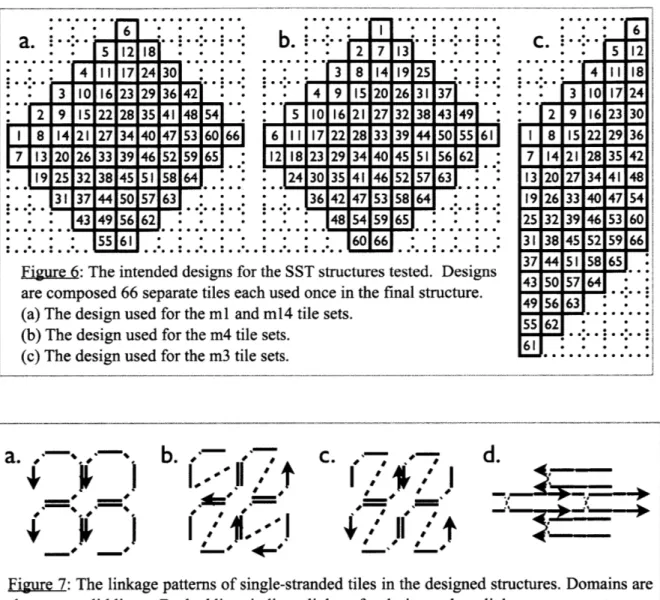
10 3 16 6 12 17 23 18 24 30 29 36 15122128135141 421 48 54: r- - - - - - - -- - -= 14121127134140147153 44 49 55 50 56 61 57 63 62

b.

11 5

11218

I40

O455156621

14I30I35I4146Is215713J.

Figure 6: The intended designs for the SST structures tested. Designs are composed 66 separate tiles each used once in the final structure. (a) The design used for the ml and m14 tile sets.

(b) The design used for the m4 tile sets.

(c) The design used for the m3 tile sets.

C. -

12i

b.

I

C.

4F7j(7t

d.

Figure 7: The linkage patterns of single-stranded tiles in the designed structures. Domains are shown as solid lines. Dashed lines indicate linkers for designs where linkers are present. (a) Four tiles in the ml or m14 structures. The junction is equivalent to a multibranched loop.

(b) Four tiles in the m4 design; (c), four tiles in the m3 design. The four-tile junction in both

designs is distinct from that in the ml design.

(d) Eight tiles in the ml0 design. The connectivity of the ml0 design differs substantially

from the other designs, incorporating a crossover and using two strands in the basic unit tile.

a.

1

1

17

11

varied domain length ml_9mer m1 ml_13mer ml-6mer ml_19mer ml_21mer ml_8mer_10T ml_9mer_10T m1_10mer_10T ml10T ml_13mer_10T

varied linker length ml_1T

ml_2T ml_4T

ml_7T

mllOT ml_13T

varied connectivity ml/m14 ml1OT/m14_1OT

m3 m3_10T

m4 m4_10T

varied sequences m1 m10 m14_10T m4_10T

m14 mlOhighGC m14_1OT_lowGC m4_10T_split Table 1: Design variables in the SST system and resulting tile sets tested. Tile sets listed within the same cell can be contrasted for comparisons across that variable. Some tile sets are

listed more than once. Table 2 contains additional information on the tested designs.

Tile assembly experiments

Myhrvold et al. measured the assembly rate of various tile sets over a range of

temperatures [35]. In these experiments, all strands of a single tile set were added to a single

reaction mixture (200 nM of each tile type to 0.5x TE buffer supplemented with 10 mM Mg2+).

The mixture was then held constant at a set isothermal temperature for 1 hour2, the assembly

period, and was then placed at 4*C for the remaining steps.

The reaction mixture was loaded into an agarose gel and underwent gel electrophoresis, which separates the structures present by their size (directly related to charge) and their degree of

folding (fully folded structures are compact compared to aggregated or partially formed structures, and so should exhibit high gel mobility). The assembly yield was calculated using band densitometry: a high-mobility band presumably indicating the folded structure was located on the gel. The amount of DNA in this band, from band density, was divided by the total amount

of DNA in the gel lane, from total lane density, to determine the calculated yield. Note that the yield as defined by this method is higher than the yield as defined by the percentage of starting

DNA incorporated into correctly assembled structures: structures with high mobility are likely to

be substantially "correct" but need not be perfectly assembled, and monomeric strands remaining after assembly may have been run off the end of the gel and as such are not accounted for.

To verify that high-mobility bands on the agarose gel did in fact correspond to fully assembled structures, reaction mixtures were adsorbed onto a surface for atomic force microscopy. Though limited detail into the tile makeup of these structures can be gleaned from such methods, but the structures formed appear to generally follow the design pattern, albeit with a substantial degree of shape heterogeneity.

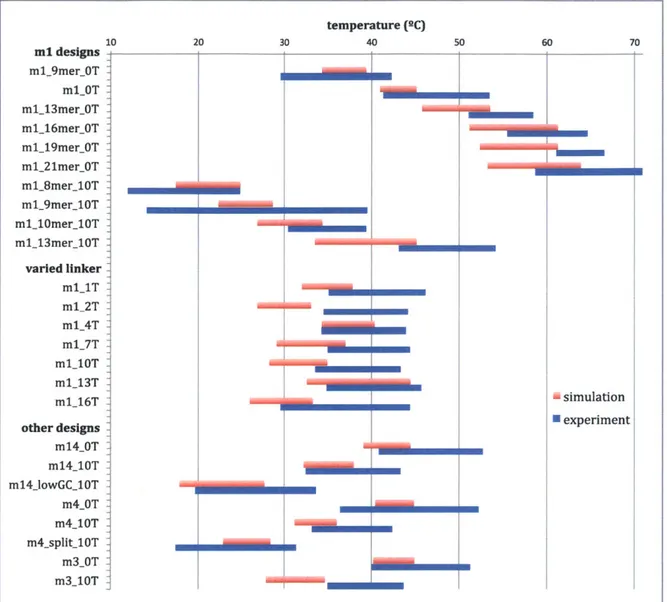
Each tile set underwent assembly reactions in parallel at different temperatures. These temperatures typically spanned about a 20'C range, with data points separated by around 3"C. A Gaussian curve was fit to the data, which was displayed as assembly yield versus isothermal assembly temperature. The peak and full width at half maximum of this Gaussian fit were calculated and given as the mean and spread of the isothermal assembly temperatures.

3.2 Results from the SST System

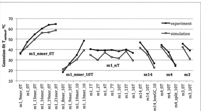
The isothermal temperatures at which peak assembly was observed to occur were directly related to predicted tile domain-domain binding strength and inversely related to the presence of a single-stranded linker region between tile binding domains. Most aspects of the analysis below are unique to this work, as domain-domain binding strengths were not previously calculated.

Domain-domain binding strengths for a design are closely and directly correlated with its optimal assembly temperature, as would be expected. The relationship is strongest when considering the melting temperatures of the domains as predicted from the nearest-neighbor model for DNA duplex melting temperatures [47], and factors that influence this calculated duplex melting temperature are predictably related to the observed temperatures for SST tile design optimal assembly. Increasing domain length is positively correlated with optimal assembly temperature, expected since longer domains have higher melting temperatures, directly

correlated with GC content in binding domains, and negatively correlated with a domain

incorporating a single mismatch, expected since this destabilizes domain duplex pairing.

The link between linker status and optimal assembly temperature is strong: the presence

of a linker shifts optimal assembly temperatures downward for a design by about 8"C relative to

a linkerless design. Curiously, there is a minimal observed relationship between the length of the

linker region and designs' optimal assembly temperatures. The trends between linker presence

and optimal assembly temperature cannot be explained by differences in stacking effects, since

the coaxial stacking lost through inclusion of a linker is largely compensated for by dangling-end

stacking of the linker region against the two adjacent domains. A more plausible explanation is

that the observed relationship is due to an entropic effect. Linkerless designs are not forced to

constrain the ends of a relatively flexible region, which would be expected to contribute a

destabilizing entropic penalty in a folded structure.

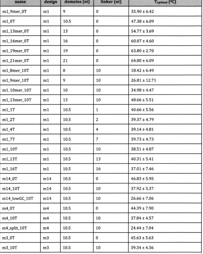
mlOT m1 10.5 0 47.38 ± 6.09 ml_l3mer_OT m1 13 0 54.77 ± 3.69 ml_16mer_0T m1 16 0 60.07 ± 4.60 ml_19mer_0T m1 19 0 63.80 ± 2.70 ml_21mer_0T m1 21 0 64.80 ± 6.09 ml_8mer_10T m1 8 10 18.42 ± 6.49 ml9mer_10T m1 9 10 26.81 ± 12.71 mll10merl10T m1 10 10 34.98 ± 4.47 ml13mer_10T m1 13 10 48.66 ±5.51 mlT m1 10.5 1 40.66 ± 5.56 m1_2T m1 10.5 2 39.37 ± 4.79 ml_4T m1 10.5 4 39.14 ± 4.81 ml_7T m1 10.5 7 39.73 ± 4.73 ml_10T m1 10.5 10 38.51± 4.87 ml_13T m1 10.5 13 40.31± 5.41 ml_16T m1 10.5 16 37.01 ± 7.46 m14_OT m14 10.5 0 46.83 ± 5.95 m14_10T m14 10.5 10 37.92 ± 5.37 ml4jowGCUOT m14 10.5 10 26.66 ± 7.06 m4_OT m4 10.5 0 44.39 ± 7.90 m4_10T m4 10.5 10 37.84 ± 4.57 m4_split_10T m4 10.5 10 24.44 ± 7.04 m3_OT m3 10.5 0 45.63 ± 5.63 m3_10T m3 10.5 10 39.34 ± 4.36

Table 2: Isothermal assembly temperatures and design features for the SST system. Data

shown are given in Supp. Info. 2 of

[35].

3.3 Implementation of the iTAM

The iTAM model was implemented for this work in Python as a Monte Carlo algorithm

and run using representations of the 25 tile sets of the SST system as input. The assembly

conditions used were those present in the physical system: 10 mM Mg2+, 200 nM each tile, and

the temperature experimentally used. Assembly times were 1 hour for most tile sets and 12 hours

for tile sets with domains > 16 nucleotides in length, as was used for the experimental system. A

fuller description of the program is given below, and a link to the program files is provided in the

supplemental material.

Tile-tile standard free energies and Mg2+ correction

In a step preparatory to running the simulation, the free energy of interaction between

each pair of domains in the tile system was calculated. This was done using a program

("feedermg.py," see supplemental) that took as input text files containing the tile set's sequences

as given in Suppl. 2

[35].

The spacing of binding domains along these designs' sequences was

hard-coded into the program. When the sequences were read from text files, the program

extracted the binding domains' sequences and wrote them to a separate list 220 entries in length,

for the 220 domains present per tile set.

These 220 sequences were read into the UNAFold program in a pairwise fashion [49].

Using UNAFold's "melt.pl" script, the standard enthalpy and entropy of binding for the

minimum free energy structure in which the two strands are bonded is computed.

This

calculated entropy value, set by default to be that for DNA in a 1 M NaCl solution, is then

corrected by the "feedermg.py" program using equation 22 in Owczarzy et al. to account for the

0 M NaCl, 10 mM Mg2+ experimental conditions [48]. This correction is most significant when

considering domains with domains 13 nucleotides or greater in length, and strengthens binding.

The output is a 220 x 220 matrix in which each entry is a pair (AHij, ASij) giving the enthalpy and

entropy of interaction between domain i and domainj under experimental conditions.

Secondary structure correction of tile-tile free energies

The domain-domain energies calculated by UNAFold and subsequently adjusted do not

account for secondary structure features that impact the overall structure's energetics. This is not

a minor effect: the enthalpies and entropies calculated by UNAFold do not distinguish between a

structure with 10-nucleotide linkers or without such linkers. Such a change is experimentally

observed to shift the assembly temperature of a design by about 6-9*C

-

quite significant when

peak assembly for these designs occurs only over a 5"C range.

To account for such effects, the iTAM model performs energy corrections based on the

tile structure design. Ideally, energy corrections would be performed dynamically during the

simulation based on the secondary structures present at each step in the assembly. The iTAM

implementation of these corrections uses a simpler scheme: domain-domain energies are

assigned an energy penalty before the beginning of the simulation that is based on the secondary

structural elements created by the formation of such bonds within the context of an otherwise

fully-assembled structure.

The iTAM accounts for the secondary structure in designs with no linkers or with linkers

52 nucleotides in length by considering that when these designs assemble, they form structures

patterned with four-arm junctions, also known as multibranch loops: see Figure 7. (Technically,

this is only true for the ml and m14 designs: as shown in Figure 7, the m4 and m3 junctions

possess distinct designs, but are treated identically for simplicity.) Each internal tile contributes

corners toward 4 separate junctions, and so removing it from a fully assembled structure

eliminates four junctions. Because tile-tile energies in this model are assigned at the domain

level, this four-junction penalty is distributed evenly between the four domains of the tile: one

four-arm junction penalty (+1.6 kcal/mol for a 0-nt linker) is assigned per domain [47].

This rule is modified for edge tiles that contain 1, 2, or 3 domains. Tiles with 1 domain

will not form additional loops on binding and do not contribute additional secondary structural

features.

Consequently, interactions involving a domain of a 1-domain tile are assessed no

secondary structure penalty. Tiles containing two domains contribute toward the formation of

only a single junction in the final assembled structure. This single junction-formation penalty is

divided between 2 domains, for 0.5 junction penalties per domain, for all interactions involving

2-domain tiles. 3-domain tiles appear only in the m3 designs, and are assigned 1 junction penalty for interactions with 4-domain tiles (for consistency) and 0.5 junction penalties for interactions with 3-domain tiles such that 3-domain tiles correctly contribute toward 2 junctions in the fully assembled structure.

Designs with linkers >2 nucleotides in length form junctions that are similar in connectivity, but experimental evidence for assigning energies to such expanded junctions is lacking. Instead, the iTAM model assigns penalties to these structures by considering that forming a domain-domain bond within a fully-assembled structure produces two single-stranded regions that are bound at both ends by double-stranded regions, which is also the case in an internal loop. Accordingly, domain-domain pairings are penalized as though they created internal loops. For an internal tile, the penalty is 1 internal loop per domain-domain pairing (+4.9 kcal/mol for a 10-nt linker) [47]. Edge tiles create fewer internal loops, as was previously the case with junctions, and fractional internal loop penalties are assigned for domain-domain pairings involving such tiles as in the junction case.

This overall treatment of tile-tile binding energies requires the following assumptions:

i. The minimum free-energy structure for domain-domain pairing predicted by UNAFold makes sense within the context of the overall tile structure. This will be the case for correct domain-domain pairs, which are most important for simulating tile assembly.

ii. The energy of the minimum free-energy structure is accurate. Melting temperatures as predicted by the nearest-neighbor model are typically around ±2*C of experimentally measurements, placing a bound on the accuracy of assembly temperature predictions [47].

iii. Each domain-domain interaction can be treated independently of its environment; overall energies are simply the sum of domain-domain energies, with the domains as defined. The formation of DNA secondary structures violates this assumption, and (as seen through the inclusion of linkers) has a considerable effect on binding energies. The secondary structure

adjustment to domain-domain energies attempts to correct for this violation to allow tiled

structures' accurate simulation by a kinetic tile assembly model.

Simulation

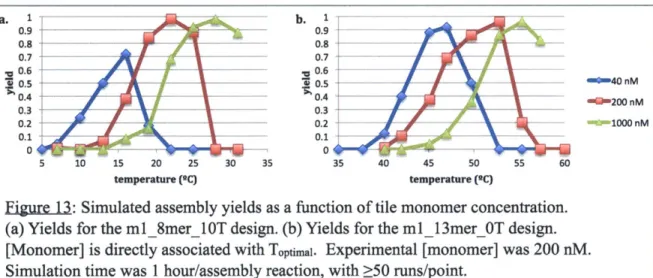
The main program, "itam.py," took as input a tile set name, set of temperatures for assembly, entropy/enthalpy values, and simulation-specific parameters such as the number of tile assembly runs to perform at a specific temperature (nruns) and the simulated tile cutoff value for halting simulations. Experimental values for the temperature, tile concentration (200 nM for all simulations), and time given to run the assembly reaction (1 hour for most tile sets, 12 hours for tile sets with domains > 16 nt) were used unless otherwise specified.

When run, itam.py began by importing the relevant list of tileset enthalpy/entropy values and calculating the 220 x 220 matrix of tile-tile interaction AG values, as described above. The simulation was initialized by selecting a tile at random from the tileset, assigning it a random rotation, and placing it onto a grid. The simulation was then run as described in sections 2.2 and

2.3. No tile was designated fixed, though the structure was not allowed to shrink below size 1.

If a dissociation event broke the structure into two discontiguous blocks of tiles, the smaller of those blocks was deleted.

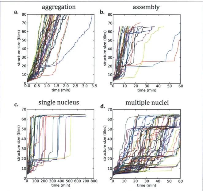
A simulation was run until any one of three stopping conditions was met:

i. The structure was of size 66 tiles and had no free edges for further tile addition. If this stopping condition was met, the simulation was ended and a structure was considered to have successfully assembled.

This condition does not require that the structure be error-free, but it does effectively require that the structure consist of a single "domain" of tiles aligned per the design layout. Simulating such structures for the full time period studied experimentally substantially increased computation times and did not obviously alter simulation results.