Computational Methods for Higher Real
K-Theory with Applications to tmf.
by
Michael Anthony Hill
A.B. Harvard University 2002
Submitted to the Department of Mathematics
in partial fulfillment of the requirements for the degree of
Doctor of Philosophy
at the
MASSACHUSETTS INSTITUTE OF TECHNOLOGY
June 2006
( Michael Anthony Hill, MMVI. All rights reserved.
The author hereby grants to MIT permission to reproduce and
distribute publicly paper and electronic copies of this thesis document
in
1.1virlhrlan r
V LJLUI% I.Lin reor''
111 XH u. .A
i1t-'
+ar
-OF TECHNOLOGY JUN 5 2006 LIBRARIES Ar.L . 1 ... .. ... . .
Department of Mathematics
/
'f
May 1st, 2006
Certified
by
...
.
...
.
...
~' 'MWhael J. Hopkins ARCHIVES
Professor of Mathematics, Harvard University
Thesis Supervisor
Accepted by
...
...y
Pavel Etingof
Chairman, Department Committee on Graduate Students
Computational Methods for Higher Real K-Theory with
Applications to tmf.
by
Michael Anthony Hill
Submitted to the Department of Mathematics
on May 1st, 2006, in partial fulfillment of the requirements for the degree of
Doctor of Philosophy
Abstract
We begin by present a new Hopf algebra which can be used to compute the tmf homology of a space or spectrum at the prime 3. Generalizing work of Mahowald and Davis, we use this Hopf algebra to compute the tmf homology of the classifying space of the symmetric group on three elements. We also discuss the E3 Tate spectrum of
tmf at the prime 3.
We then build on work of Hopkins and his collaborators, first computing the Adams-Novikov zero line of the homotopy of the spectrum eo4 at 5 and then
gener-alizing the Hopf algebra for tmf to a family of Hopf algebras, one for each spectrum eopl1 at p. Using these, and using a K(p- 1)-local version, we further generalize the
Davis-Mahowald result, computing the eop_1 homology of the cofiber of the transfer
map BEp -+ So.
We conclude by computing the initial computations needed to understand the
homotopy groups of the Hopkins-Miller real K-theory spectra for heights large than p- 1 at p. The basic computations are supplemented with conjectures as to the collapse of the spectral sequences used herein to compute the homotopy.
Thesis Supervisor: Michael J. Hopkins
Acknowledgments
I begin by thanking my advisor, Mike Hopkins, for putting up with me for almost 6 years now. From helping me with my undergrad thesis, to helping me decide what
to do after graduation, to never suggesting that a project I was interested in was not
neat or interesting enough, Mike has been a fantastic advisor from the start. I will certainly miss our meeting come next year.
I next wish to thank my parents, Drs Ellen and Kelly Hill. While they possibly never understood my fascination with all things mathematical, they were nonetheless
incredibly supportive of it, driving me to math competitions and classes at LSU
when I was younger and spending inordinate sums on math texts. I would not be
here without their support.
My dear and incredible friends also deserve recognition. First to my Harvard friends, notably the Amys, the Adams, Fancy, and Cliff. They definitely got me sanely through Harvard. Next comes my new MIT crowd: Teena, V, Mark, Bridget, JNKF, Marco, Chris, Andre, Nora and Francesca. MIT has been a wonderful experience, largely due to you. I wish also to acknowledge the help and support of Haynes Miller who always allowed me to crash other people's meetings with him because I might
find it interesting and who carefully read this thesis.
Lastly I come to perhaps the most important acknowledgments: Bridge and Tim. Bridge and I have technically known each other since college, but it was only in graduate school that I learned what a fun and fantastic person she really is. Oddly enough, she accepted my suggestion that we live together, and she has been the best roommate I could ask for.
It is to Tim that I dedicate this thesis. He has been unfailingly supportive, he has been incredibly compassionate during this ordeal, and he has made me blissfully happy these past three years. I would not have lasted here without him.
Contents
1 Introduction and Applications 1.1 Introduction ...
1.1.1 Chromatic Height 2 and tmf ....
1.1.2 Heightp-1 at p ...
1.1.3 Higher Heights ...
1.2 Applications of the Computations ....
1.2.1 The tmf and EOp-1 Hopf Algebras 1.2.2 The Homotopy of eo4 ...
The 3-local tmf homology of
2.1 Organization of Chapter . 2.1.1 Conventions and No 2.2 Fundamental Hopf Algebra
2.2.1 The Adams Spectral 2.2.2 The tmf Hopf Algelt 2.3 Review of ko,(fRP ) . . .
2.3.1 General Results and 2.3.2 The ko homology of
2.3.3 Computing ko(IRP°
2.4 The tmf Homology of the (
2.5 The tmf Homology of P° 2.6 The tmf Homology of the F
2.6.1 The Skeleta of R 2.6.2 The Skeleta of P° 2.7 The 3 Tate Homology of t
BE3 15
... ...
15
tation ... 15
... ...
16
Sequence for R-modules ... . 16
ora ... 16
. . . 20
Definitions . . . 20
R ...
20
) ... ... 21
3ofiber of the Transfer P - So ... 22
. . . 24
inite Skeleta of R ... . 25
. . . 25
. . . 32
mf ... . 32
3 The 5-local Homotopy of eo4 3.1 Organization of the Chapter ... 3.2 The Geometric Model for EOp-1 ... 3.2.1 The Moduli Stacks Used ... 3.3 Rational Computations ... 3.3.1 Rational Information ... 3.4 Statement of the Main Result ... 3.5 Preliminary, Prime Independent Remarks. . 3.5.1 Computation of H*(A/Ipi, FlIp-) 2 11 . . . .11 . . . .11
... ..
12
. . . . 13... ..
13
... ..
13
... ..
14
33 . . . .33 . . . .33 . . . .34 . . . .36 . . . .36 . . . .37 . . . .37 . . . .38 . . . . . . . . . . . . . . . . . . . . . . . .3.5.2 Computation of H*(A/Ip_2, F/Ip-2)
3.5.3 Computation of H*(A/Ip_3, F/Ip-3)
3.6 Computation at the Prime 5 ...
3.6.1 Computation of H*(A/11
, F/I)
. ..3.6.2 Computing H*(A/Io, /I0) ...
3.6.3
H*(A,
) ... ..
3.7 Adams Differentials and the 5-local Homotopy 3.8 Formulas Relating the classes Ai ...
4 The eop_1 Hopf Algebra
4.1 Introduction ...
4.2 A New Spectrum ...
4.3 Hopes for eop_1 ...
4.4 The eop_1 homology of BEp ... 4.5 The EOp-1 homology of BEp ...
4.6 Charts for Computing Ext at 5 ...
. . . . of eo4 . . . . . .. . . .. . . ..
5 Cohomology of Z/pk with Applications to Higher K-Theory
5.1 Introduction ...
5.2 The Structure of S(kppl) ...
5.2.1 Computation of the Tate Cohomology ... 5.2.2 The Higher Cohomology of Z/p ...
5.2.3 Concrete Example with H° Information ... 5.3 Applications to Higher Real K-Theory ...
5.3.1 Height k(p- 1) for k<p... 5.3.2 Height p(p- 1)...
5.4 Recent Work and Indications of Future Developments ... 5.4.1 Ravenel's Work and Hopes for Elements ...
6 A Computational Lemma for Differentials in Spectral Sequences
6.1 Introduction ...
6.1.1 Organization ... 6.1.2 Conventions ...
6.2 Higher Differentials out of Lower Ones ... 6.2.1 Main Result ...
6.2.2 Variants of the Lemma ...
6.2.3 A Massey Product Lemma for Massey Products ... 6.3 Applications. ...
6.3.1 Kraines' Results on Massey Powers ...
...
38
...
38
...
40
...
40
...
42
...
44
...
45
...
46
47...
47
...
47
...
49
...
51
...
51
...
53
55 55 55 56 56 57 57 58 58 59 60 61 61 61 61 61 61 62 64 64 64List of Figures
The Adams E2 term for tmf.
ExtA(l). (F3, 3) . . . . .
Ext Gr(A)(F3, F3) ...
May E2 page for ExtA(F3, F3)
ExtA(1). (F2, Gr) ...
ko(P
)
...
ExtA (F3, H*(R)) ...
The Long Exact Sequence for Ex The Adams E2 term for tmf, (RI
The Long Exact Sequence for Ex The Adams E2 term for tmf (RI
The Long Exact Sequence for Ex The Adams E2 term for tmf, (RI
Long Exact Sequence for Ext(Mg The Adams E2 term for tmf, (R['
H*(A/Ip_ 3, r/Ip_ 3) . . . . .. E1 page for H*(A/I1, F/Il )..
The E2 page for H*(A/I 1, F/I1)
H*(AI1, r/Il) . .. . . . .
E1 page for H*(A/Io, r/Io)..
E2 Page of H*(A/Io, r/Io)
E1 Page for H*(A, F) ...
4-1 The Ring ExtA(l). (F5, 5) .. ...
4-2 The Spectral Sequence for ExtA(l).E(a 2)(F5, F5)
4-3 The Spectral Sequence for ExtA(1)*.E(a 2, 3)(F5, F5)
4-4 The Spectral Sequence for ExtA(1).0E(a2,a3,a4)(F5, F5)
2-1 2-2 2-3 2-4 2-5 2-6 2-7 2-8 2-9 2-10 2-11 2-12 2-13 2-14 2-15 3-1 3-2 3-3 3-4 3-5 3-6 3-7 . . . . .. . . . 16 . . . . .. . . . 18 . . . . .. . . . 19 . . . . .. . . 19 . . . . .. . . 21 . . . . .. . . 21 . . . . .. . . 23 . . . . .. . . 27 . . . . .. . . 27 . . . . .. . . 28 . . . . .. . . 28 . . . . .. . . 29 . . . . .. . . 30 . . . . .. . . 30 . . . . .. . . 31 40 41 41 42 43 44 44 53 53 54 54
...
...
...
...
...
...
...
. . . . . . . . . . . .Chapter 1
Introduction and Applications
1.1 Introduction
In this thesis, we will develop and analyze various computational tools to better understand the Hopkins-Miller higher real K-theories EO,. The Hopkins-Miller the-orem produces for each finite subgroup G of the extended Morava stabilizer group,
Gn, a spectrum EO,(G) which sits between the Lubin-Tate spectrum En and the
K(n)-local sphere [18]. These spectra serve as useful approximations to the very complicated K(n)-local sphere, and for small values of n, they have been beneficial in producing small resolutions of LK(n)S°, allowing for a relatively complete
under-standing of the homotopy [6, 13, 16]. However, for n > 2, the homotopy groups of EOn are largely mysterious. One of the goal of this thesis is to provide a complete description of the homotopy ring of EO4 at the prime 5, indicating how the
com-putations work at larger primes. Building on this, we provide a new Hopf algebra suitable for computing not only the homotopy ring of EOp_1 at p, but also the EOp_1
homology of any space, knowing only the homology of the space as a comodule over the dual Steenrod algebra.
1.1.1 Chromatic Height 2 and tmf
The case of n = 2 is well studied. Using the machinery of elliptic curves, Hopkins and his collaborators produced a global spectrum tmf that K(2)-localizes to EO2 at 2 and at 3, where in each case, we take a maximal finite subgroup of 62 which
contains a maximal p-subgroup [19]. The spectrum tmf has several advantages over the spectra EO2, in that it is an f.p. spectrum in the sense of Mahowald and Rezk [24]
and the homotopy ring is finitely generated over Z. Moreover, the close connection between elliptic curves and tmf allows one to show that there is a Hopf algebroid for computing tmf homology using the Weierstrass form of an elliptic curve. However, in practice, this is difficult to use at best.
Hopkins and Mahowald showed for tmf at 2 there is an Adams spectral sequence for computing tmf homology similar to that for ko.
Theorem (Hopkins-Mahowald). There is a spectral sequence of the form
ExtA(2).
(F2,
H(X))
>tmf(X )
for cell complexes X.
For primes bigger than 3, there are similar results, using the splitting
tmfw V Fp()BP (2),
where p(k) and the number of wedge summand are determined by the combinatorics
of tmf .
Davis and Mahowald have computed ExtA(2). for a large number of spaces,
includ-ing truncated projective spaces [8]. At the time, many of these computations were viewed as academic exercises, since Davis and Mahowald thought that there was no
spectrum with cohomology A//4(2) [10].
The computational machinery established by Davis and Mahowald can also be modified using filtration arguments similar to those of Chapter 2 to prove results
similar to the following.
Proposition. As graded groups and as modules over Z[C4],
7r*(tmftE2) = II 8k ko.
The missing piece of the computability puzzle for tmf is what happens at the
prime 3. The form of the Hopf algebra required for the Adams spectral sequence was conjectured by Henriques and the author and is proved in Chapter 2. Results similar to those of Davis and Mahowald are also proved in Chapter 2, together with a result analogous to the previous proposition.
1.1.2 Heightp-1 atp
For n > 2, there is a geometric model similar to that of elliptic curves which was developed by Hopkins, Mahowald, and Gorbounov. It provides a Hopf algebroid analogous to the Weierstrass Hopf algebroid and will be discussed in Chapter 3. This Hopf algebroid was used by Hopkins to show that the higher Adams-Novikov filtration elements of 7r, EOp_1 are very simple. Moreover, it can be used to compute the entire
Adams-Novikov zero line, producing a complete description of the homotopy algebra. However, this computation is quite lengthy and is worked out in full only for the prime 5 in Chapter 3.
While the Hopkins-Gorbounov-Mahowald Hopf algebroid is useful in proving re-sults about the homotopy of EOp_1 and has been used by others to prove results as
diverse as the non-existence of certain Smith-Toda complexes [28], it is not well suited to doing actual computations of the EOp_1 homology of spaces or spectra.
Addition-ally, the spectra are K(p- 1)-local, making their homotopy algebras complete local rings. In Chapter 4, we discuss an analogue of tmf for height p - 1 at the prime p.
We then prove results analogous to those of Chapter 2 for both a conjectural connec-tive f. p. spectrum eop-l and for the non-connecconnec-tive, non-K(p- 1)-local spectrum eopl [A-']. Applications of such a computation are also included, demonstrating the ease of use of the techniques.
1.1.3 Higher Heights
Most of the previous discussion has involved the spectra EOp_l at the prime p. For larger heights divisible by p- 1, very little is known about the spectra EOn. The maximal finite subgroups of Gn are known by a theorem of Hewett [15], but the com-plexity of the action of G on 7rEn has prevented actual computations. In Chapter 5, we work out some of the higher cohomology of 7//p with coefficients in a distinguished module, the symmetric powers of a direct sum of copies of the reduced regular repre-sentation. Devinatz and Hopkins has shown that as a 7//pk-module, r.Epk-i(p_l) has
a filtration such that the associated graded is essentially the symmetric algebra on the reduced regular representation for this group [12]. Restricting to the copy of Z/p
reduces the computation required to the computation we present. This computation
should provide a basis for future work on the higher homotopy of EOn beyond the current knowledge of EOpl.
1.2 Applications of the Computations
1.2.1 The tmf and EOp_
1Hopf Algebras
Mahowald's computation of ko,(RP ° ) has proved useful in a variety of contexts at
the prime 2. In particular, Mahowald used ko,(RP n) and ko,(RP°/RPk) to get
infor-mation about v1 metastable homotopy theory in the EHP sequence [23]. Mahowald
has also used ko,(RP °°) to detect elements in his rj family [22]. At the prime 3, the
role of the spectrum ko is most naturally played by the spectrum tmf. To generalize these results of Mahowald's, the initial piece of data needed is the tmf homology of
BE3.
A theorem of Arone and Mahowald shows that v. periodic information is captured by the first pf stages of the Goodwillie tower [3]. This recasts Mahowald's result from [23] into a more readily generalizable form. To get v2 periodic information at the prime 3, the initial data needed comes in part from QS° and Q(BE33 ), where BE3'
is a particular Thom spectrum of BE3. Just as Mahowald uses knowledge of the ko homology of stunted projective spaces to reduce the questions involved to ones of J homology, we hope that a similar analysis, using Behrens' Q(2), spectrum will allow an analysis of the v2 primary Goodwillie tower at 3 [6].
Minami shows that the 3 primary T7j family will be detectable in the Hurewicz
image of the tmf homology of the n-skeleton of BE3 for appropriate choices of n
[27]. While determining the full Hurewicz image is a trickier task, understanding the groups and simple tmf operations on them could help determine if the conjectural Tb
Minami actually shows that for all primes p > 2, the Tj family will be detectable
in the Hurewicz image of the eop_1 homology of an appropriate skeleton of BEp. The computations in Chapter 4 provide a starting point for applying this program.
1.2.2
The Homotopy of eo
4The computation has two main immediate applications. The first is the interest in its own right: this solves an invariant problem considered "bad" by algebraists in a way that allows similar analysis for other metacyclic groups. The second, perhaps more interesting, application is to the existence of self maps realizing multiplication by vk on the Smith-Toda complex V(2) at the prime 5.
This story has many antecedents. Hopkins and Mahowald used the spectrum
tmf and computations in its homotopy to correct a result of Davis and Mahowald,
showing that the complex M(1, 4) at the prime two has a self map that induces v232 multiplication in K(2)-homology [17, 9]. Behrens and Pemmaraju demonstrated the similar results at the prime 3, again using tmf to show that V(1) has a self-map inducing multiplication by v in K(1)-homology [7]. The methods of Chapter 3 lend themselves to computing the eo4 homology of V(2) at the prime 5. By using tricks similar to those employed by Hopkins-Mahowald and Behrens-Pemmaraju, we should be able to compute the appropriate power of v3 which exists on V(2) at 5.
Chapter 2
The 3-local tmf homology of BE3
2.1 Organization of Chapter
In §2.2, we introduce the main computational Hopf algebra A, Ext over which is the Adams E2 term for computing tmf homology. In §2.3, we review Mahowald's computation of the ko homology of RP°°, presenting it in a manner which can be most readily generalized. In §2.4, we carry out one of the computational steps analogous to Mahowald's, computing the tmf homology of the cofiber of the transfer map, and in §2.5, we complete the computation of tmf.(BYE3). Rounding out the computations, in §2.6, we compute the tmf homology of the finite skeleta of R, giving additional results about that of the finite skeleta of BE3. The last section presents conjectures
as to further results. A computation of the homotopy of the E3 Tate spectrum for
tmf is presented in §2.7.
2.1.1 Conventions and Notation
We restrict attention to the prime 3 and assume that all spaces and spectra are 3-completed except in §2.3. For ease of readability, let H be HZ/3. If X is a space or spectrum, let X n] denote its n-skeleton.
For ease of readability, we also will write P° for BE3. If we are dealing with a
truncated classifying space with cells between dimensions n and m, we will write the
spectrum as pm .
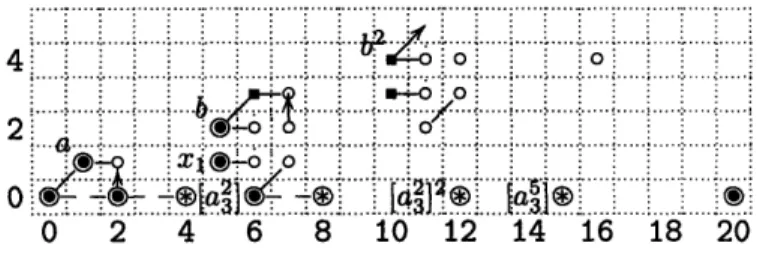
Finally, we need some tmf specific notation. To describe it, we begin with a picture of the Adams E2 term which we will derive in §2.2 in which all of the elements in
question will be labeled (Figure 2-1).
Let I denote the ideal of the Adams E2 term for tmf. generated by v, 4 and c6.
Let denote the ideal of tmf. generated by 3, 4, 6, and their A and A2 translates. I is the annihilator ideal of the elements ca and /. For brevity, the reader is asked to always assume the relations I = 0 and I/3 = 0 in all Adams E2 terms, unless
explicitly stated otherwise. Moreover, the relation c3-C2 = 27A always holds and
... ... ... ... ... ... ... | B. w. w @ w w ... 6w 6
6 : . . . . .. ... ... ... ... .. . ... .. ... ... . ... L
24
6
8 .1012 4 618.
:eAdams t 2 erm for t...
2.2 Fundamental Hopf Algebra
2.2.1
The Adams Spectral Sequence for R-modules
We begin by quickly reviewing the variant of the Adams spectral sequence we will use. Most of the statements are immediately provable using Adams' original work, and full details can be found in [4].
Let R be an Eo~ ring spectrum, and let E be an Aoo R algebra (ie an Ao~ monoid in the category of R modules). For any R module M, we can cosimplicially resolve M using E in the category of R modules, just as with the ordinary cosimplicial Adams resolution over the sphere spectrum. In other words, we can form the cosimplicial spectrum i.. .... ... ...; ...; ;;
EARS ARM :=EAR M EAR EARM ===. ··
as with the ordinary Adams resolution. . . .. . .. ... . .. . .. . .. . .. . .. .. .This cosimplicial resolution gives rise to a
.
.. . .. . .. . . . . .. ... . . . . . . .~~~~~~~. . . . .. ... . .. ... . . . ...
0 2 4 6 8 to 12 14 16 18 20 22 24
FigBousfield-Kan
spectral sequene 2-1:of the Adams tfor tmf
2.2
Fundamental Hopf( Algebra
M))
(M).
2.2.1We again call this spectral sequence the Adams spectral sequence. Again, just asR-modules We begin by quickly reviewingth the variant of theary if have certain flatness assumptionsllAdams spectral sequence, we
usthen we can identifyof the staE tents are immediately stprovable result, we need 2 a sm' originall bit of,
notation: Let R l etails can be foundote be an E. ring spectrum, and let in [4]. E be an A. R algebra (ie an A monoid
Proposition ategory 2.2.1. of R modules). For any n E module, the n (Ecosimplicially resolve HopfMa
algebroid and the Adams E2 term is
Ext
(E.,s.s)
(E., E.M).As we shall see, the Hopf R malgebroid (Es, EjustE) ioften is quite cosimpliciale to work with.Adams
resolution over the sphere spectrum. In other words, we can form the cosimplicial
spectrum
E AR-AR M= E AR M
E AR EAR M
2.2.2 The tm f ERHopf AR M
is the
Enilpotent completion of
M, , jusbraas with the ordinary Adams resolution. This cosimplicial resolution gives rise to a Bousfield-Kan spectral sequence of the form
Tot(7r,(E AR' AR M)) =4
7r.(ME)-We again callpply the machinery of the previous sectioral sequence the Adams spectral sequence. Agatmf, to E = H,just and
wiM =th tmf A X. The Adams spectralum H made is an E into tmf algebra by coassumposing thes,
then we can identify the E2 term. To cleanly state the result, we need a small bit of
notation: let ERM denote 7r*, (E AR M)
Proposition 2.2.1. If ERE is flat as an E module, then (E., ERE) is a Hopf
algebroid and the Adams E2 term is
Ext
(E* ERE) (E.,E*
M).As we shall see, the Hopf algebroid (E., E RE) is often quite simple to work with.
2.2.2
The tmf Hopf Algebra
We apply the machinery of the previous section to the case R = tmf, E = H and
zeroth Postnikov section of tmf with the reduction modulo 3. In other words, we take
the composite
tmf - HZ
H.
Since each of these is a map of Eo~ ring spectra, the composite is. Moreover, since every module is fat over H, we need only identify
A := Htmf H.
Theorem 2.2.2 (Henriques-Hill). As a Hopf algebra,
A
= A(1)*0
E(a2),where a2 = 9, and A(1) = F3 []/6l 0 E(0o, l) is dual to the subalgebra of the
Steenrod algebra generated by 3 and Pl. The elements in A(1)* have their usual coproducts, and
A(a
2) =
1®a
2+
rl
T(
1- 2()
+
a2 1.
Proof. We begin with an observation of Hopkins and Mahowald, as formulated by
Behrens [6]. If we let
C = So UcI e4 Uc
1 e8,
then smashing with tmf gives
tmf A C
=tmf
0(2),
where tmfo0(2) is an Eoo ring spectrum corresponding to elliptic curves together with a choice of an order 2 subgroup. As an algebra,
,r*(tmfo(2)) = Z3[a2, a4],
where a2 = vl and a = v2 modulo (3, v1) [6]. The ideal (3, a2, a4) is a regular ideal,
and we can pass to the quotient of tmfo0(2) by it in an A, way, realizing H as a
tmfo0(2) spectrum [2].
Spelled out more cleanly, we have realized H as the cofiber of the map a4 on the
spectrum tmfo0(2) A V(1).
To finish the proof, we smash this cofiber sequence with H over tmf, giving the cofiber sequence
]8H Atmf (tmfo(2) A V(1)) -4 H Atmf (tmfo(2) A V(1)) H Atmf H.
We begin by analyzing the homotopy of the first two tmf modules in this resolution:
r*
(H Atmf (tmfo(2)A V(1))) = H, (C A V(1); Z/3).The structure of this as a graded vector space is that of A4(1)*. Since A is a commutative Hopf algebra, the Borel classification of Hopf algebras over a finite field ensures both that a4 is zero in homology and that the structure of this as an algebra
is as listed [26]. This follows from considering the degrees of the elements, since odd elements must be exterior classes and the element in degree 4 must be the generator of a truncated polynomial algebra.
Since the unit map S - tmf is a 6-equivalence, the natural map
HAso H
H
AtmfH
is a 6-equivalence. This implies that the induced map in homotopy is a Hopf algebra isomorphism in the same range, and this gives the coproducts on the elements r0, r
and f.
To determine the coproduct on a2, we will endow A with a filtration such that a2
is primitive in the associated graded. This filtration gives rise to a spectral sequence
EXtGr,(A)(F3, IF3) * EXtA(F 3, F3)
converging to the E2 term of the Adams spectral sequence which computes 7r,(tmf).
We shall use the known computation of r(tmf) to deduce differentials in this alge-braic spectral sequence, and this will determine the coproduct on a2.
We first filter A by letting A(1), have filtration 0 and letting a2 have filtration 1.
The initial piece of data needed is the cohomology of A(1). As an algebra
EXtA(l). (F3, IF3) = IF3[VOV,3
vo
= 2 =0,
12 =VO).
This is pictorially represented in Figure 2-2.
... ... ' ... ... ... ' ... ].. ... ... r... ...1...'... ... ;...' .... . ... ?... ... .... :.:.:.:.:.:.:.:.:.: 7 ... ... ~~~~~~~~~~~~~~~. . .. . .. ... ... ... :.: : .. . : ... : ... : . ..: :..:..: . . . ... ...: *1. ....I .. . ... . ... ... ... . . . . .. ... ... ... ... i .i i ~ ~ ! ! i i !. ; ~ !i ~ i ! ! ! i .. i !.. ; , j i . .... i
.. .... ... ...
...
... ... ... ..
... ...
...
...
: : .: , : ] : : : · · · ... *I ,. ... . ... ... ...o
' ... ... ... ' ... .... ... ... ... ... ... ... ; _ ... ... ... .... ... ... ... ... 2 . ... . ... . . . ... .. . . ... .. . . . ... ... ...-.... ... ... 1 ~~~~~~~~~~~~~~~~~~~~~~~~~~~~~~~~~~~~.. ... ... ... b,, 0 2 4 6 8 10 12 14 16 18 20 22 24 26 28 30 Figure 2-2: ExtA(l). (F3, F3)Since a2 is primitive in the associated graded Hopf algebra, we know that EXtGr(A) (F3, F3) = ExtA(l). (F3, F3) [4].
This Ext group is the E1 page of a spectral sequence converging to the Adams E2
term ExtA(F3, F3). Since there is nothing in dimension 7 in tmf*, we know that the
element a2 must be killed. The only possible way for to achieve this is for dl (c4) = 2
!
li
0 2 4 6 8 10 12 ..14 14 16 16 .18. 18 20 .. .. 22 24 26 28 30. .. .. . . .. ... . .. .. .. .. .. .. .
Figure 2-3: ExtGr((A) (F3, 3)
At this point, we rename some of the remaining elements:
c4=vo C4, C6 = V1, =4 .
Lemma 6.2.1 gives the d2differentials:
d2([a242]) = v3, and d2([vo42]) = V3a. The E2 page with the d2 differentials is included as Figure 2-4.
.,'" ""' ...
. 6 4 . . ·... ... 2 0 ..0246
.. A , :4D: i,,. :, ... 8 . . . . 'i' .. .. . . ... .Z . . . .. .. .. i... ~ : :i : : ... 2 C--6 444 . . . ~~[hour
]
10 . 1 · . .. .... : . .... .. .. ... : . .. ... 10 12 14 16 18 . ' - ... "n ... 4C65 . '... ..... . .. ...
...
:...
....
20 2 2 2 28 :3 22. '2'4 . ... . 22 24 26 28 30Figure 2-4: May E2 page for ExtA(F 3, F3)
For the d to have the appropriate form, we must have
4(a
2)
=1
a2+ a
2(
10l
1-12
To).
If the sign is negative, then we can simply replace a2 by -a 2 to correct this. []
One can ask if there is a formal group interpretation to the Hopf algebra given in Theorem 2.2.2, similar to the interpretation of the Steenrod algebra as the auto-morphisms of the super additive formal group. This seems to be the case. If E is an elliptic spectrum, then the homotopy groups of E Atmf E are the automorphisms of the formal group of E that extend to automorphisms of the associated elliptic curve. For the case E = H, we can proceed only by analogy, since the additive elliptic curve
8 6 4 2 0 .s.
is not in the moduli stack used in the construction of tmf. However, if we consider the automorphisms of the additive formal group which extend to automorphisms of the additive elliptic curve, then we reconstruct the truncated polynomial part of Theorem 2.2.2. We conjecture that a full results can be recovered by considering super formal groups and super elliptic curves.
Corollary 2.2.3. There is a spectral sequence with E2 term
EXtA
(F3,
H.(X))
converging to the 3-completed tmf homology of a space or spectrum X.
2.3
Review of ko,(RP
°°)
In [21], Mahowald uses the homology of cofiber R of the transfer map BE2 -+ So
to compute its ko homology and the ko homology of IRPo. Since the method we will employ to handle tmf,(BE3) is similar, we quickly review Mahowald's technique here. For this section only, all computations will be done at the prime 2.
2.3.1 General Results and Definitions
The homology of R sits as an extension of the homology of ERP by the homology of S°, and let ei denote the generator of Hi(R). The coaction of the dual Steenrod algebra on H,(R) is determined by the comodule structure on H,(FEP °O) and the
coaction formula
P(e2) = 2 e + 1 e2.
Let A(1) be a spectrum whose cohomology is a free A(1)-module of rank 1. Smash-ing A(1) with ko gives a presentation of HIF2 as a ko-module spectrum. Applying the Adams spectral sequence machinery introduced earlier reestablishes the following classical result, normally proved using a change of rings argument.
Proposition 2.3.1. There is a spectral sequence converging to the ko homology of a
space X with E2 term ExtA(l), (F2,
H,(X))
2.3.2
The ko homology of R
Mahowald's key observation was that there is a filtration of H,(R) such that the associated graded is a sum of comodules over A(1), whose Ext groups are easy to compute.
Proposition 2.3.2. There is a filtration of H,(R) such that the associated graded is
00
Gr= Gr(H*(R))
= 4kM
k=0 where M is the A(1), comodule A(1)* OA(0), F2.
The proposition shows that if we compute Ext of Gr, then we see that it is torsion
free, with a Z in dimensions congruent to 0 mod 4 (Figure 2-5). :11,11.11", 1.1,111:1 : ' .... ' ... i.... '1 1 ... '.. .... .... 1 ' 1: 1 1..1' i 1 .... 11:' ... ... .... 1: 1 , .... I. ... ... ...'.. . .. . ... ...:, ... ... ... ...'..! ... ... ... . ... 64 : . ... ... ... ... · . ... . .. .... , ... . . ... ' ... ... . . ... . ... ... ... ... ... ... ... ... 6~~~~ 4 .. .. .... ;... . . . .. 2 . ,. . . l
i
o ;i... ... ... ...i'i.... ... !.... - - - .- - ..8....S...!...^...---! -... ' .. .... : .... ... ... .... .... .... ... .... .'. ..- .... .... ... .... 'l' .... .... ... .... 0 2 4 6 8 10 12 14 16 18 20 Figure 2-5: Ext.A(). (F2, Cr)Since this is concentrated in even degrees, both the algebraic extension spectral sequence and the Adams spectral sequence collapse. There are non-trivial extensions, though, as a ko,-module.
Lemma 2.3.3. As a module over ko.,
ko.(R) =Z2[y]
Remark. This lemma shows that Mahowald and Davis' result in [11] that ko A R
splits as a wedge of copies of HZ is not true in the category of ko-module spectra.
2.3.3
Computing ko,(IRP
c)
Computing ko,(RP') requires looking at the long exact sequence in ko homology for the cofiber sequence
SO--+ R -+ ERP '.
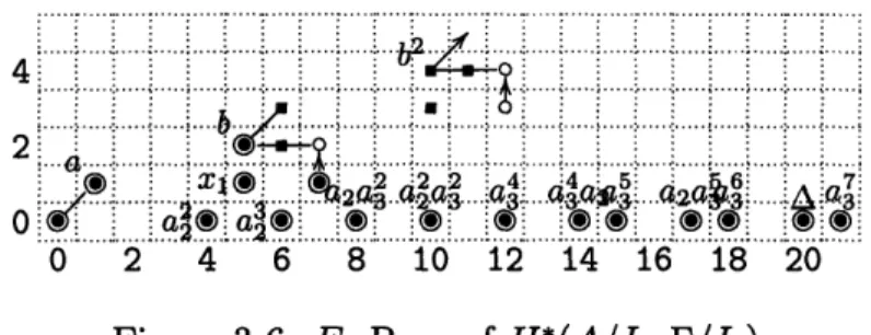
The first map is the inclusion of the zero cell, and takes 1 to 1. From this, the result is easily determined (Figure 2-6).
... ... ... ... i ... 4 ... ... ... ... :...:... ... ... ":... .... ". ... : ... : " ~~~~~~~~.... ... 0...:...:...:.... :... ... .... ... ... :.... :...:... .... .. ... ... i... i... .... .... -...: 0 2 4 6 8 10 12 14 16 18
Figure 2-6: ko,(llP
~)
~~~~~~~~~~~~~~~~~~~~~~~~~~~~~~~~... ~.X_..4 :
. . . ., . . . .,. .. . . . .. . . . .* ... ... ,... . . . . .. . .. . ... . ... . . ... .. .... .. .. . . ... .. . . .. .... . ... .. . .... . . . ... ....:. , ... ... ...-.t .l ... ... .... ... .... ... ... . 2 6 . 12 ; 14 16 : Figure 2-6: ko* (RP°°)2.4 The tmf Homology of the Cofiber of the
Trans-fer P
S
o
Homologically, the situation at the prime 3 is analogous to the computation at 2.
Let R denote the cofiber of the transfer map P - S. The homology of R sits as an extension of the homology of EP' by the homology of S°, and again let ej denote the generator of Hi(R). The coaction of the dual Steenrod algebra on H,(R) is determined by the comodule structure on H(EP) and the coaction formula
b(e4) = - e 1 ® e4.
The tmf analogue M is again the comodule A4(1)0A(0). F3, where A(O) is the
exterior algebra on the Bockstein.
Lemma 2.4.1. H.(R) admits a filtration for which the associated graded is
00
Gr(H*(R))
=1
2kMk=O
Proof. The -kth stage of the filtration is given by taking the subcomodule generated
by the classes in dimensions 12n + 1 for all n > k. An elementary computation in the cohomology of the symmetric group shows that the associated graded is exactly what is claimed.
Lemma 2.4.2.
EXtA(F3, M) = F3[O0, 64].
Proof. To prove this lemma we apply a long sequence of spectral sequences. First
filter A as before by letting A(1)* have filtration 0 and a2 have filtration 1. This
filtration extends to a filtration of M in an obvious way, letting M have filtration 0, and we have a spectral sequence
Extcr(A) (F3, M) = ExtA(F3, M).
As a Hopf algebra, Gr(A) is very simple: the algebra structure stays the same, and now a2 is primitive. Now we can use the two short exact sequences of Hopf algebras
A(1)* -+ Gr(A4) - E(a2) and E(a2) - Gr(A) -- A(1)*
to get a spectral sequence that converges to this Ext group and starts with
EXtE(a2) (3, ExtA(1). (F3, M))
A final change of rings argument shows that
and this forces the result in question, since the target of any differential on the polynomial generator is zero for degree reasons. LI
Since this algebra is concentrated in even degrees and since each of the graded
pieces starts an even number of steps apart, the spectral sequence starting with Ext
of the associated graded for H,(R) collapses (Figure 2-7). There are non-trivial extensions. '...~' ... 8: i 6
4~~~~~~~~~~~~~~~~~~~
2 0 0 2 4 6 8 10 12 14 16 18 20 22 24 26 28 Figure 2-7: ExtA (3, H.(R)) Lemma 2.4.3. 00EXtA (F3, H*(R)) = IF3 [Vo, 64] el2k/C6el2k = Voe12(k+1).
k=O
Proof. We show this by returning to the cobar complex. Since the homology of R
has the very simple pattern of copies of M connected by a To comultiplication on the top class in each hitting the bottom class in the next, it will suffice to show that in the first copy, c6 on the 0 cell is cohomologous to 27 on the 12 cell.
For simplicity, we will let i denote the class in dimension n in M. In the cobar complex for ExtA(1). (F3, M), there is an element 16 such that
X16= To T TO i13 + ... and d(x16) = c6 io.
The class x16 can be found by considering the Ext implications of the short exact
sequence of comodules:
F3{io, i4, i8} -+
M
--+
F3{i5, i, i13}.When we add in the next copy of M, we change the coproduct on i3 to
(i13) =
(1
®i
9+60i
5+1
i8 + T
1 ®i4+2
1®io+
1
i
13)
+T
0i
12-This is the only change to the coproducts in our comodule, so when we consider again x1 6 and take its boundary, the only change is the addition of terms coming
one coming from To0 0 T i13, so the real boundary is
d(x
6)
= C6i +
T0 To0
To0
i12.In other words, c6 on the base class is (up to a sign) v3times the class in dimension
12. E
Theorem 2.4.4. The Adams spectral sequence for the tmf homology of R collapses,
and as a tmf,-module,
tmf.(R)
= Z3[3,
].
Proof. The Adams E2 term is concentrated in even topological degrees, and this implies the collapse of the Adams spectral sequence. The previous lemma solved the extension problem, and the proof of Theorem 2.2.2 shows that c4 gives the element
CA
3.
2.5 The tmf Homology of P°
The most difficult of the computations now behind us, we can compute the tmf homology of P 0 by simply considering the long exact sequence induced by applying
tmf, to the cofiber sequence
SO R poo.
The first map is the inclusion of the zero cell into R, and so this map in tmf-homology just takes 1 to 1. Since this is a map of tmf,-modules, we see immediately that this map is injective on elements of Adams-Novikov filtration 0, with image
3 [ 413 , C6,
[3A],
[9A21 [ 4A, ][3A2], [c4A2], [CA,[c
6A],
[c6AC 2], A3] /(27 (7 = c3-C6) C C c3[3 2717] . Additionally, since a and /3 act as zero on all of the classes in tmf,(R), the kernel of this first map is the submodule of tmf, generated by a, 3 and their A translates. These together establish the following theorem about the tmf homology of EP'.Theorem 2.5.1. The tmf homology yPo sits in a short exact sequence
0
- Gn - tmfn(EP') tmf _1 - 0,where tmf._ 1 is the subgroup of tmfn_1 of Adams-Novikov filtration at least 1 and
Gn,
the cokernel of the map tmfn - tmfn(R), is given byZ/3
ffm=lZ/36m k- _, 2
mod3,
i + j =O
fk 7Z/36m+3j+i k- 0 mod 3
(Mm=O"/
G24k+12j+8i-
~k
/3 6m+3j+i k1
2 mod 3 i +j >O'
where j < 2, and i < 3. The sequence is split as a sequence of groups. There is
a hidden a extension originating on the copy f 32 in tmf20 and hitting the Z/3
summand of G24.
Proof. This short exact sequence is just a restatement of the earlier comments about
the long exact sequence in tmf homology. It is split because the elements coming from
Gn have Adams-Novikov filtration 0, and the convergence of the Adams-Novikov spectral sequence ensures a map of groups from tmf*(EPOO) to Gn which is a left inverse to this inclusion.
The structure of the groups Gn is easy to show. A basis for tmf (R) is given by the collection of monomials of the form Aki6E, where i < 3, and 27E6 = 6, 3 4= C4.
This is simply because if we can solve the relation on A in tmf (R). A basis for the Adams-Novikov filtration 0 subring of tmf, is given by the monomials
Akc6c fork-- 0 mod 3 or k =- 1, 2 mod 3, i + j >0, [3A]Ak, and [3A2]Ak
Recalling that
Akcc = 33J+iAk
and collecting all terms of the same degree yields Gn.
The hidden extension can most readily been seen by considering the long exact sequence in Ext induced by the cofiber sequence. In this situation, A from the ground sphere kills A in the Adams E2 term for tmf,(R), and a32 on the ground
sphere survives. O
Remark. The proof of this theorem also shows that the transfer induces a bijection
between the elements of higher Adams-Novikov filtration of tmf, and the elements
of tmf,(P°) of Adams-Novikov filtration at least one (together with the Z/3 coming from the 3-cell). This exactly repeats the situation at the prime 2, where the transfer
maps the higher Adams-Novikov elements in ko,(GRP°) bijectively onto those in ko.
2.6 The tmf Homology of the Finite Skeleta of R
For completeness, we include the tmf-homology of the finite skeleta of R. These computations serve as starting points for the program of Minami to detect the
3-primary
m
family [27].2.6.1 The Skeleta of R
Let n = 12k + i, for 0 < i < 12. We wish to compute the tmf-homology of R[n. Lemma 2.6.1. There is a filtration of H,(R[12k+i]) such that the associated graded is
k-1
\
Gr(H*(R[12k+i])) ( E12nM) G E12kMi,
where Mi is the subcomodule of M generated by all classes of degree at most i for
i < 12, and M12 is M9 plus a primitive class in dimension 12.
Proof. The required filtration is just the restriction of the filtration used in the proof
of Lemma 2.4.1 to the subcomodule H,(R[l2k+il). 0 The comodules Mi are the homology of R[i], and this splitting result and the follow theorem demonstrates that knowing their tmf-homology gives that of all finite skeleta. The proof of Theorem 2.4.4 shows the following
Theorem 2.6.2. As a module over tmf.,
tmf*(R[12k+i]) = Z3
[3]
{eo, .e12.. ., e12(kl)}(
AMiel2k/(c6el2j - 2 7e12(j+l)),where Mi is the tmf-homology of spectrum R[i.
The remainder of the section will be spent computing the modules Mi. To save space, in what follows we use two indices: which ranges from 0 to 2 and e which ranges from 0 to 1. When these appear, it means that all possible values of the index are actually present.
Proposition 2.6.3. The spectra R[1], R[2], and R[3] are simply So. This implies that
Mi = tmf*, 1<i<3.
Lemma 2.6.4. The spectrum R[4] is the cofiber of
a,.
The tmf-homology of this isthe extension of the module generated by [eo] and [e 4] and subject to the relations
a[cae4] = 3eo, a[Aeo] = - 2[a0e4], ae0 = 3[Aeeo] = I[ae4] =
B4[ae4]
by the module
7Z3[c4, c6, A]{[3e4], [C4e4], [c6e4]}.
The extension is determined by the two relations
c4[3e4] = 3[c4e4] ± c6eo, c6[3e4] = 3[c6e4] ± c4e0.
Proof. Since the spectrum M4 is the cone on a1, we can use the long exact sequence in Ext to compute the Adams E2 term (Figure 2-8).
As a module over the Adams E2term for tmf*, this E2 term is the extension of
-3[Vo, 4, C6, A, 3]{eo}
by
F3[vo, c4, C6, A]{[voe4], [ 4e4], [ 6e4]} ( F3[A, 3]{[ae4]},
subject to the relations
8
. . ....
6 4~ ~~~~~~~~~¶ 20~~~~~~~~~~~0
...~~~~~~~~~~~ ~ ~ ~ ~ ~ ~ ~ .. . . ... ... .4.M ... .. '. -- ..' : ' ..:... .... i, :.~~~~~~~~[:4e ... ... ... "'"':: ... ... ... ...0
0:
2 4 6 8 10 12 14 16 18 20 22 24 26!
28Figure 2-8: The Long Exact Sequence for Ext(M4)
and depicted in Figure 2-9.
6
Thsasspectral
sqec oh seuecsaseta oueovrteAassetae
d
2(
() =a
32d
3([aA
2])
=305,
imply that Aeo and /. 2eo are d
2 cycles and that the following differentials hold:
d2(L\[Ce4]) = 3'eo, d3(oA2 [ae4]) = /35[ae4].
This last d3 implies that in fact,
d3(A2eo) = 0[el
using the relation involving a multiplication on 4 3 ae4]. L
Lemm .The spectra 1, .[6. ..and "':e ... cb o ... e ...
.... ... .. . :... .. .:... .. : .. ... ... ... : .. - . .. . . . : . ... .. .. ..
0 2 4 6 8 10 12 14 16 18 20 22 24 26 28
Figure 2-9: The Adams E2 term for tmf,(R[4] )
This Adams spectral sequence is a spectral module over the Adams spectral se-quence f the tmf-homology or of the sphere, and the Adams spectral sequence for the sphere,
d2(a\) = a/32, ¢3([at2]) = ¢,)
imply that /Aeo and A\2eo are d2 cycles and that the following differentials hold:
d,(a\[og4]) = ¢¢0o, d3(al/¢[~¢4]) = ¢5[a4].
This last da implies that in fact,
d3(A\2eo)=
_-/410e4],using the relation involving oa multiplication on [ae4]. 0] Lemma 2.6.5. The spectra R[5], R[6], and R[7] are the coibet of the extension of ae
over the mod 3 Moore spectrum. The tmf -homology of these spectra, Mi is the tmf , module generated by
and subject to the relations
o3e5] = i3[3eo], 4] = eo, a[Aeo] [[oe= 0. e4
(a,133)eo = ([ae4], [e 5]) = 34[ae4] = 0.
Proof. In the long exact sequence in Ext induced by the inclusion of the 4-skeleton
into R[5], the inclusion of the 5-cell kills the element [voe4] (Figure 2-10).
'- :' -itt .... i ·
'
...
... ,'
:
T
: ':...i
+. : :i.,.,...',.T.+'
.-<. . .. .. ... · . ... .. ... .. ... .. ... -. . . . .. 1 ... . 1 . .14. 2 4 6 8 10 12 14 16 18 20 22 . A . : I i .. . : : 4 4 . . . . : : A 4 ... *` . : " . . . . ... 24 26 28Figure 2-10: The Long Exact Sequence for Ext(M5)
The elements [c4e4] and [c6e4] survive, and the relations in the Ext term for the 4-skeleton ensure that in the Adams E2 term for M5,
vo[c4e4] = 6eo, vo[c 6e41] = Ceo.
Moreover, since a and fi multiplications on the class [vOe4] are trivial, the classes [aes]
and [3e5] survive to the Adams E2 page (Figure 2-11).
6
4
2 0:4 I I I I : I I.I
...
0 2 4 6 8 10 12 14 16 18 20 22 24Figure 2-11: The Adams E2 term for tmf,(R [5 ])
A computation in the bar complex establishes that
vo[ae 5] = C4
eO-This shows that the Adams E2 page, as a module over that for tmf,, is
F3[vo, c4, C6, A, ]3{eo, [4eo], [eo], []e4, [/e 5]}
/(a[oe4] -- ,3eo, [c4 eo] -LV 0 o[3e5] aeo, I([3e51, [e4]))
8 6' · I 4 2 0 0 26 28 I I I . .... .. ... .. ... .. I . : I : : I
!-I-*. - :
IThe differentials again follow from those in the Adams spectral sequence of tmf.
L
At this point, the patterns of extensions and differentials repeats. This makes the
final computations substantially easier.
Lemma 2.6.6. The spectrum RN8] is the spectrum C from§2.2, where the middle
cell is replaced by the mod 3 Moore spectrum. The module M8 sits in a short exact
sequence
0 - tmf,{[3A 6eo], [ A6 eo], [ 6eo], [3es]/((a, /3)([eA 6eo], [A6 eo]), I[fes])
-
Ms
-+ 3[c4, C6, A]{[3e8], [ 4e8], [6es]} 0,where the extension is determined by the two relations
c4[3e8] = 3[c4e8] ± c4[3eo], C6[3e8] = 3[c6e4] ± C4[ 3eo].
Proof. The long exact sequence in Ext coming from the short exact sequence in
homology induced by the inclusion of R[ 5] into RI81 is determined by the connecting homomorphism which takes e8 to [ae4] (Figure 2-12). The linearity of this map shows
... . . . .. . . . ... .... ... ... .; .. . .. ... . . . . ... .:. 10 1 . .. . .. . .. . . ... ... . ;. ... ... .. ... ... ... .... ..14 16 18 20... 14 16 18 .. .. ... 20 .. .. . . . . .. ... .. 22 24 26 28
Figure 2-12: The Long Exact Sequence for Ext(Ms)
that the Adams E2 term for M8 (Figure 2-13)is an extension of
3[Vo C4, c6, ]{eo, [ eo], [ 3eo]} D3[A, 3] 0 E(a){[/3e s]} by
F3[Vo, C4, C6, Al]{[voes], [c4e8], [ 6e8 ]},
subject to the extensions
c4[voe8] = Vo[c4es] + c43e0, c6[voe8] = Vo[C6es] + 6
3e.O-The differentials are again determined by those of tmf*. 3e.O-The only classes which support non-trivial a multiplication are multiples of [e 5], and here, the differentials
8 6 : 4 2 . 0 0 . . o
[-
e5.
[v0e8 .2 4 6 8 1 12 14 16. .
Go2 4 6 8 10 12 14 16 18 20 22
. ! Zi
24
.... 28';
.. .
Figure 2-13: The Adams E2 term for tmf (R[8I])
are the same as for M5:
d2(Ai[Oe5]) = io 2Ai-l [/e51, d3([aA2][/e5]) = 35 [fe5].
El
Lemma 2.6.7. The spectra R[91, R0], and RI"] are the cofiber of the may from E4C(a) to C which is multiplication by 3 on the 4 and 8 cells. The module M9 can
be expressed via the short exact sequence
0 -* tmf{[aeg]} -+ M -* z3
[4]eo
-+ 0,{[ ]} [C4]~[
where the only extension is given by
c6eo = 9[oe9].
Proof. The cofiber sequence coming from the inclusion of RM8] into R[9] induces a long exact sequence on Ext (Figure 2-14). The connecting homomorphism is
eq [voe8] + [3eo]. 8 4 ., .. . ... ! .:... 0 2 4 6 r t .. . . .. . . .. 1 . .. 1 8 ... . ... . . 2 14 16 18 20 22 24 26 28
Figure 2-14: Long Exact Sequence for Ext(M9)
This is a map of modules over the Adams E2 term for tmf,, and just as before,
the element [ae9] is in the kernel of this map. This gives hidden extensions analogous
8 6 4 2 0 0
to the ones for M4 and M5 in the Adams E2 term for Mg:
a[ae
9]
=/3e
5,vo[ae] = [eo].
The c4 and c6 extensions coming from [voes] give two more extensions:
vo[c4e8] = c4[3eo], vo[C6es] = c4[ eo].
This establishes that the Adams E2 term is given by the extension of
F3[oV, C4, C6, [eg]
by
¢2 F3[Vo, C4, C6, ]{eo, [Feo], eo]},
where c6eO = v2[ae9] (Figure 2-15).
8...
6 ', 4 t, 2024
i~~
~~~~.
1 [~~ .. ... ... .... ..~~~~~~~
.. .. ,. . :~~~~~~~~~~~ . . . . 6 8 10 12ae 1] 4 16 18 6 8 10 12 14 16 18 . . . .. . . . .... . ... .. . . .... . ... . 20 22 24 26 28Figure 2-15: The Adams E2 term for tmf (R[91)
Just as before, the ordinary Adams differentials determine the differentials,
recall-ing that [-eo] = [eg]:V
0
d2(Ak[=eo]) = k 2A-l[eo] = 2[,e5], d3(A2[e5]) = [].
The Adams differentials here preserve the exact sequence, and this establishes the
statement of the Lemma. O
Remark. For completeness, we note that if it were possible to include a 13-cell,
attaching it to the 9-cell via a, then the attaching map in long exact sequence in tmf
homology would take the copy of tmf, coming from the 13-cell isomorphically onto the factor tmf,{[aeg]}.
Proposition 2.6.8. Since the twelve dimensional class is primitive in M12, we
con-clude that as a tmf.-module,
2.6.2 The Skeleta of P°
The analysis of the preceding section allows us to completely determine the structure of the groups tmf (Pn). However, due to the complexity of the combinatorial prob-lem, explicit demonstration of these groups in unenlightening. We instead present the following theorem concerning bounds on the orders of these groups.
Theorem 2.6.9. If n = 12k + i, then 33k+2 annihilates the torsion subgroup of
tmf,(Pn). Moreover, if i > 5, then there are elements of order exactly 33k+1, and if
i > 9, then there are elements of order exactly 33k+ 2 .
Proof. This is immediate with the consideration that the large torsion subgroups are
generated by high powers of 2. If we consider only a finite skeleton of POO, then we
27
include only finitely many powers of this element. The largest such element occurs in dimension 12k. If i is at least 5, then we have the element 3 on this element. If i is
3
2
at least 9, then we have the element i on this element. These provide the elements
of exact order. [
2.7 The
3
Tate Homology of tmf
The analysis used to compute the tmf homology of R applies to compute the homo-topy of
tmftE3 = E (tmf A P°°)_oo = lim (tmf A P).
A mod 3 form of James periodicity shows that as A(1),-comodules,
po
=
y]-12kH,
p-.
H* (PZ'1
2k+3) =(i3 ).
3The Adams spectral sequence argument in §2.5 shows that the map
ir, (tmf A P'12(k+l1)+3) -+ 7r, (tmf A Pc12k+3)
is surjective on the G, summand and zero on the tmf, summand. This implies that there are no lim1 terms coming from the inverse system of homotopy groups. Moreover, this is a system of tmf,-modules, and considering the action of c4 and c6
in each of the modules in the inverse system allows us to conclude
Theorem 2.7.1. The homotopy of the E3 Tate spectrum of tmf is an indecomposable
tmf, module, and
1r(tmftEa
)
- 3 34
63where
I is
the ideal in 7ro(tmft 3) generated by elements of positive Adams filtration.
Chapter 3
The 5-local Homotopy of eo4
3.1 Organization of the Chapter
In §3.2, we review the Gorbounov-Hopkins-Mahowald Hopf algebroid and the stacks associated with it. In §3.3, we apply the techniques from the previous section to compute the rational homotopy of eop_1. In §3.4, we state the theorem which the
rest of the chapter will be spent proving. The middle sections of the paper compute the Adams-Novikov E2 term for the homotopy of eo4, loosely following Bauer's
com-putation of the 3-local homotopy of tmf [5]. We introduce the Bockstein spectral sequences needed for computation in §3.5, and we carry out the prime independent computations. In §3.6, we restrict attention to the prime 5, competing the compu-tations for eo4. We try to present proofs that follow formally from Massey product
considerations, and if we have not included proofs of any required lemmas, we also include proofs from the bar complex. Finally, in §3.7, we compute the Adams differ-entials.
3.2 The Geometric Model for EOp-1
The success of the geometric model of elliptic curves for building a geometric model for EO2 and for building a connective version eo2 leads to a search for analogous
models for primes bigger than 3.
Manin showed that the Jacobian of the Artin-Schreier curve over p
yp-1 = XP-
Xadmits a formal summand of height p- 1 [25]. Since this is the first interesting height at the prime p, Hopkins, Mahowald, and Gorbounov used this fact to build a geometric model analogous to the story of elliptic curves and tmf at the prime 3, and they show that the formal completion of the Jacobians of the family of curves over
W(pP-l )
carries the Lubin-Tate universal deformation of the Honda formal group, together with an action of Z/p M Z/(p- 1)2, a maximal finite subgroup of Gp_1 [14]. Such
curves are non-singular if the discriminant A of the polynomial
xP + alx P -1+ + ap
is a unit.
The scaling action on the Artin-Schreier family given by Equation 3.1 allows us to split off a graded Adams summand. This splitting is algebraically realized by considering Equation 3.1 as a homogeneous graded equation, where xl = 2(p- 1),
IyI
= 2p, Ir = 2(p- 1) and ai = 2i(p- 1), and the A action fixes the graded pieces.The degree of the discriminant is 2p(p- 1)2.
3.2.1 The Moduli Stacks Used
Lurie's derived algebraic geometry produces sheaves of Eoo ring spectra over various moduli stacks associated to this family of curves. Since the global sections are all closely related, we briefly introduce the stacks involved. In all cases, stackification takes place in the flat topology. Since this is not the topology to which Lurie's machinery applies, we show that there are natural tale, affine covers. We first note that curves of the form given by Equation 3.1 are corepresented by the graded Hopf algebroid
(A, F) = (Zp[al, ... , ap, A[r])
The first stack considered was the stackification of the Hopf algebroid associated to corepresenting non-singular curves of the form given by Equation 3.1, completed at the maximal ideal I of the degree zero part. In other words, the stack we consider
is
Mp-1 Stack(Proj(A[A-1]'), Proj(F[A-1]A)).
This is essentially the stack first considered by Hopkins, Gorbounov, and Mahowald, as it singles out the height p- 1 information, and the global sections of the sheaf associated to this stack is the K(p- 1)-local spectrum EOp_1 described earlier.
Part of the power of Lurie's machinery is that we can weaken the conditions on our stack, looking not only at a formal neighborhood of the maximal ideal of the degree zero part but rather at the entire ring corepresenting non-singular curves of the form given by Equation 3.1. Better said, Lurie's machinery produces an appropriate sheaf of Eoo ring spectra Op-1 over the stack
Apl = Stack(Proj(A[A-]), Proj(Fr[A-])).
The global sections of this sheaf is an HFp local spectrum denoted eopl[A- 1]. It is hoped that a connective version of this spectrum can be constructed. The stack we consider is the full weighted projective space given by


![Figure 2-11: The Adams E 2 term for tmf,(R [5 ]) A computation in the bar complex establishes that](https://thumb-eu.123doks.com/thumbv2/123doknet/14437537.516316/28.918.201.718.283.471/figure-adams-term-tmf-computation-bar-complex-establishes.webp)

![Figure 2-13: The Adams E 2 term for tmf (R[ 8 I ]) are the same as for M 5 :](https://thumb-eu.123doks.com/thumbv2/123doknet/14437537.516316/30.918.203.715.108.284/figure-adams-e-term-tmf-r-i-m.webp)