Computational Photography with Novel Camera Sensors
by
Hang Zhao
Submitted to the Department of Mechanical Engineering
in partial fulfillment of the requirements for the degree of
Master of Science in Mechanical Engineering
at the
MASSACHUSETTS INSTITUTE OF TECHNOLOGY
MASS ACHUESL INSTITUTE
MAR 0
2
2016
LIBRARIES
ARCHiVES
February 2016
@
Massachusetts Institute of Technology 2016. All rights reserved.
A uthor ...
Certified by ...
Signature redacted
V
Department of Mechanical Engineering
January 15, 2016
Signature redacted
...
Ramesh Raskar
Associate Professor of Media Arts and Sciences
Certified by
Signature redacted
Thesis Supervisor
Douglas P. Hart
Professor of Mechanical Engineering
Mechanical Engineering Faculty Reader
Signature redacted.
A ccepted by
...
. . . .. . . .
Rohan Abeyaratne
Chairman, Department Committee on Graduate Theses
Computational Photography with Novel Camera Sensors
by
Hang Zhao
Submitted to the Department of Mechanical Engineering on January 15, 2016, in partial fulfillment of the
requirements for the degree of
Master of Science in Mechanical Engineering
Abstract
In this thesis, two computational camera designs are presented. They target two major goals in computational photography. high dynamic range (HDR) imaging and image super-resolution (SR). HDR imaging refers to capturing both bright and dark details in the scenes simultaneously. A modulo camera does not get saturated during exposure, enabling HDR photography in a single shot without losing spatial resolutions. The second camera achieves image super-resolution with its non-conventional pixel design. It is shown that recording multiple images with a sensor of asymmetric sub-pixel layout increases the spatial sam-pling capability compared to a conventional sensor. Both proposed camera designs are the combination of novel imaging sensors and image recovering algorithms. Their potential applications include photography, robotics, and scientific research. Theoretical analyses and experiments are performed to validate our solutions.
Thesis Supervisor: Ramesh Raskar
Title: Associate Professor of Media Arts and Sciences Thesis Reader: Douglas P. Hart
Acknowledgments
[want to express my sincere thanks to all the people who have helped me in the last two years.
I would like to thank Professor Ramesh Raskar for supervising me in the fascinating research field of computational photography. Ramesh proposed the revolutionary idea of modulo camera, which is an important topic of this thesis. During the time in Ramesh's Camera Culture group, I extended my research scope into computational cameras. com-puter vision and machine learning. I felt rewarding and fulfilling in completing this thesis, which is a condensed output of what I have studied in the Camera Culture group.
I am grateful to Dr. Boxin Shi, who has offered me a lot of hands-on help all along my study. With his rich experience in research, I learned how to explore a new area, and attack a hard research problem. His Support and encouragement in spirit also drove me forward in research.
I should thank Dr. Christy Cull, for her dedication and expertise in developing the hardware, traveling to meetings and reviewing paper drafts. We have co-authored on several technical papers, and our collaboration was a great expenence.
In addition, I enjoy the discussions with my labmates Achuta Kadambi, Professor In Kyu Park, Dr. Hyunsung Park, Dr. Barmak Heshmat and Mingjie Zhang. They have provided me with insightful ideas on my thesis. For the rest of my labmates, whom I do not mention here, it has been an enjoyable time working with all of you.
I would also like to thank Professor Douglas Hart, who is my thesis reader in the me-chanical engineering department.
Finally, I want to thank my parents, who are supporting in all aspects in life from the other side of the world. I feel blessed to have you and would like to take this opportunity to express my deepest appreciation.
Contents
1
Introduction1.1 Computational Cameras . . . .
2 High Dynamic Range Photography with a Modulo Camera
2.1 Related Works . . . . 2.2 Background . . . . 2.3 Single-shot HDR Recovery . . . .
2.3.1 Formulation of natural image unwrapping .
2.3.2 Energy minimization via graph cuts . . . .
2.4 Multi-shot HDR fusion . . . . 2.4.1 Accurate scene radiance estimation . . . .
2.4.2 Multiple modulus images unwrapping...
2.5 Experiments . . . .
2.5.1 Synthetic test . . . .
2.5.2 Real experiment . . . .
2.6 D iscussion . . . .
3 Sub-Pixel Layout for Super-Resolution with Images in
3.1 Related W orks . . . . 3.2 Good Sub-pixel Layout for Super-Resolution . . .
3.2.1 Single image case . . . .
3.2.2 Multiple images in the octic group...
3.2.3 Good sub-pixel layout . . . .
the Octic Group
13 14 17 19 20 T) 23 23 27 27 28 31 31 32 32 37 39 40 40 42 46
3.3 Reconstruction Algorithm . . . . 47 3.4 Performance Evaluation. . . . . .. . . . . 48 3.4.1 Synthetic test . . . .. . ... . . . .. . . . . 48 3.4.2 Realdata test . . . .. . . . . 52 3.5 D iscussion . . . . 53 4 Conclusion 55
List of Figures
1-1
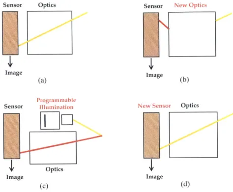
An oversimplified sketch of major components of conventional cameras (a) and computational cameras (b)-(d). Computational cameras with new optics (b), programmable illuminations (c), and new sensors (d). . . . . 152-1 A modulo camera could well recover over-exposed regions: (a) image
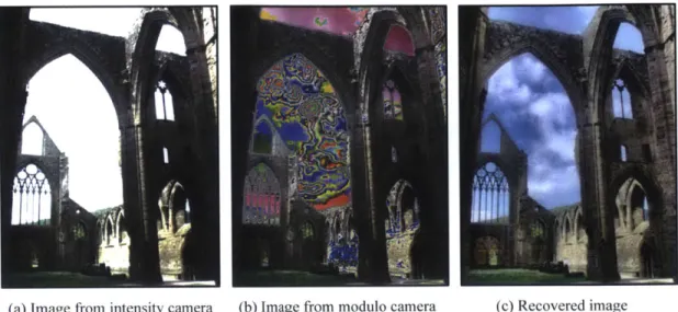
taken by an 8-bit intensity camera, the image is saturated due to the bright sky; (b) image taken by an 8-bit modulo camera, with the same exposure level as (a); (c) recovered and tone-mapped image from modulus, which retains the information in the saturated part. Radiance map is courtesy of
G reg W ard. . . . . 18
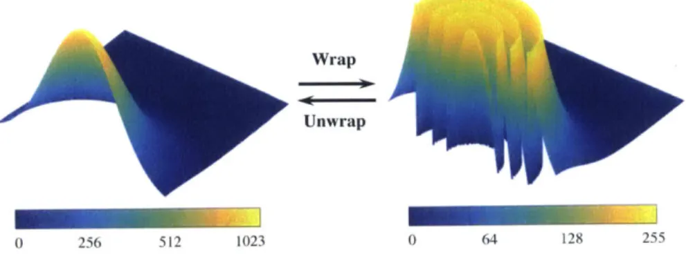
2-2 An over-simplified wrapping and unwrapping example: a surface with con-trast ratio 1023 : 1 is wrapped to an 8-bit range of a concon-trast ratio 255 : 1, and modulo fringes appear in the wrapped image. . . . . 21 2-3 Pixel architecture of the modulo sensor: pulse frequency modulator
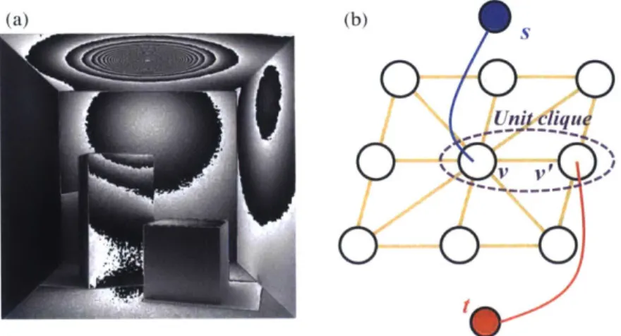
deter-mines the quantization level of the sensor. Whenever voltage passes the threshold, a counter will receive a pulse to count up. Digital signal pro-cessing control logic resets the counter to zero whenever the counter is full. 22 2-4 (a) Synthetic image of a scene taken by a modulo camera. Modulo fringes
are brought by the bright light source on the ceiling. (b) Graph representa-tion: each pixel forms cliques with its surrounding 8 pixels. Source s, sink t and an unit clique (v, v') form an elementary graph. . . . ..24 2-5 (a) The piecewise energy function to be minimized for natural HDR
2-6 (a) Intermediate unwrapping solution at each iteration: from left to right {1, 3, 10, 30}. The images are linearly scaled in intensity, where gray bars below tell the corresponding intensity values for each image; (b)
Tone-mapped image of the final result . . . ... 26 2-7 Illustration of response function I f(E) for short and long exposures.
All possible (continuous) radiance levels are shown on the bar below: (a) Intensity camera; (b) Modulo camera. . . . . 29
2-8 Comparison between multi-shot HDR using an intensity camera and a
mod-ulo camera. Under multiple exposures, reconstructions with an intensity camera suffers from severe quantization effects in high radiance areas; a modulo camera is able to reconstruct radiance with low errors in all regions. 30 2-9 Single-shot HDR recovery. Regions in the modulus images with wrapped
values correspond to saturated regions in the intensity images. Radiance
data of the first row is courtesy of Raanan Fattal. . . . . . . 33 2-10 Multi-shot HDR fusion. Close-up views highlight the visible details in
dashed squares. Quantization noise is visible in images from an intensity camera, but not in those from a modulo camera. Best viewed electronically. 33 2-11 Real experiment: single shot. The modulus image is unwrapped to become
an HD R im age. . . . . 34 2-12 Real experiment: multiple shots. Brightness is linearly adjusted for
visual-ization. After merging the short and long exposure. the details of radiance values are better preserved. . . . . 35
2-13 Failure case - synthetic data: when the local dynamic range of ground
truth is extremely huge (the region in the sun), our single modulo image unwrapping method may fail, multiple-shot recovery is required. Radiance map is courtesy of Jack Tumblin. . . . . 35 2-14 Failure case -real data: strong noise in this case is created by extending the
3-1 Existing CCD sensors with non-conventional sub-pixel layouts (bottom row). By transforming the image plane, their images in the octic group show different sub-pixel layouts, which can be combined for significant resolution enhancement (top row). The OTCCD images under 4 rotations can perform 4x SR. Comparing the OTCCD with the Super CCD, it can be seen that sub-pixels with an asymmetric layout produce more variation in their images in the octic group. . . . . 39
3-2 Different sub-pixel layouts and their HR-to-LR mapping matrices P. with magnification factor M = 2. (a) Conventional SR: LR pixels with double the size as HR pixels undergo a sub-pixel displacement: (b)-(e): examples of different sub-pixel layouts. Different color-shaded areas (RGBYW here) represent different sub-pixels, and the white area within one pixel is to simulate a gap that does not record photon charges. . . . . 40
3-3 Sub-pixel layouts with r = 5 (the gap among pixels is a dumb sub-pixel) in a sub-group of the octic group = {e, N1 N2, R3}. These layouts could build a P with rank(P) = 16. Four images captured with such sub-pixel layouts can be used to perform 4x SR. . . . . 42
3-4 Values of rank(P ) varying with different r, t, and M. Top row: t = 4: bottom row: t 8. (a) and (d) are exact values from simulation: (b) and (e) are Lipper bound from Proposition 1; (c) and (f) are 2D planar views of (a) and (d). The numbers overlaid on the matrix area of (f) indicate difference from (d) to (e) (cells without numbers mean the upper bound is reached). . 46
3-5 Simulated images under various sub-pixel layouts for 4 x SR. The rank and condition number of their corresponding P are indicated below the sub-pixel layout. (a)-(c): r = 4; (d)-(g): r = 5; (h), (i): r = 11. For each
layout, white means the dumb sub-pixel, and other colors indicate other effective sub-pixels. . . . . 49
3-6 SR results varying with sub-pixel layouts. The left most column shows the ground truth image and LR image observed by the conventional sensor with the same pixel size as our pixel. (a)-(d) here show lx SR results under various sub-pixel layouts from Fig. 3-5(a)-(d). The number below each image is the RMSE value itr.rt. ground truth. . . . . 50
3-7 (a) 4 x SR results and (b) 8x SR results with full-rank sub-pixel layouts from Fig. 3-5(d) and Fig. 3-5(h). The left most column shows the ground truth image. The LR image refers to the results from a conventional sensor. Close-up views are shown in the rightmost of each column. . . . . 5 1 3-8 SR results with noise. (a) Poisson noise with ; = 1.07 plus 8-bit
qUantiza-tion; (b) Poisson noise with r = 108 plus 8-bit quantization. Three different reconstruction methods are compared: IBP, 12-, and TV-based methods. . . 52
3-9 SR results using real data. (a) 4x SR with OTCCD sub-pixel layout in Fig. 3-1, (b) 8x SR with our good sub-pixel layout in Fig. 3-5(h). From left to right: images using conventional sensor. image views from an sensor with sub-pixel layouts, and SR result. . . . . 53
Chapter
1
Introduction
With the advances of digital cameras and portable electronics, photography has already become an integral part of modern life. Taking photos is a perfect way to record and share important moments in our daily life. However, cameras today are still far from perfect: there are much fewer images of night scenes than those taken in daytime you can find from on-line search engines, because it is way more challenging to take pictures in the dark; bulky photography equipments are still the first choice of people who want high quality photos.
Computational photography is an emerging field coming from computer graphics, com-puter vision and optics. It aims at improving image capturing or processing with digital computation. Conventional ways of enhancing cameras' imaging capabilities, like large optical lenses and tripods, brings disadvantages such as bulky sizes and increasing cost. With the introduction of computation, cameras can not only shrink in size, but also achieve features that are not possible ever before. Typical topics of computational photography in-clude high dynamic range (HDR) imaging, panorama, super-resolution, light field imaging, image-based rendering, etc.
In this thesis, two important topics in the computational photography field are explored: high dynamic range (HDR) photography [60] and image super-resolution (SR) [52, 51].
Theoretical analyses, numerical simulations, and physical experiments are conducted in the research.
and our camera design methodology.
Chapter two describes our design of a modulo camera, which is able to realize HDR imaging in a single shot without trade-offs in spatial resolution.
Chapter three describes our proposed image super-resolution technique with non-regular sensor pixel layouts.
1.1
Computational Cameras
The development of cameras has been remarkable over the last century, however, the basic components of a traditional camera remains the same. As shown in Fig. 1-1(a), a group of lenses linearly map the scenes onto the sensor/film to form an image. To improve the quality of images, conventional techniques include: (1) complicated lens designs to get rid of different kinds of aberrations; (2) semiconductor design to maximize pixel size and sensor sensitivity, etc.
Computational cameras [41, 62], a concept proposed more than a decade ago, takes a different approach. The basic idea is: modifications are made during the image captur-ing process, and more meancaptur-ingful information are recovered afterwards with computation. Therefore, it requires the co-design of hardware and software. We should note that the development of computational cameras greatly benefits from the progress in signal pro-cessing and the computation power of computers. Today the use of computational cameras is not limited to photography any more, those cameras are used widely in computer vision., robotics, medical diagnosis, biological imaging, and astronomical imaging.
In my mind, there are basically three variants of computational cameras. The first kind is cameras with new optics, shown in Fig. I-1 (b). The new optics map rays in the light field of the scene to the sensor in some unconventional fashions. The extra information provided by the new optics might include perspective views, spectral distribution, etc. One of the "star" products is light field cameras by Lytro Inc, it enables refocusing after the image is taken. Of course, refocusing is only one of the applications for light field photography. There are a lot work on coded aperture [57, 37], visual tags [381, glare removal [47], etc. Recent computational display technologies also inherit the ideas from light field [58, 361.
Sensor Optics Image (a) Irogramiii na W c Sensor
L
L
Optics Image (c) Sensor 1ww Image (b) Optics Image (d)Figure 1 -1: An oversimplified sketch of major components of conventional cameras (a) and
computational cameras (b)-(d). Computational cameras with new optics (b). programmable illuminations (c), and new sensors (d).
The second kind is cameras with active programmable illumination components, shown in Fig. -1(c). Normally, the illumination pattern is coded in a certain way that, the sensor can decode. Based on this concept, Microsoft Kinect uses synchronized infrared projectors and sensors to get the depth information of the scene. Other related works include 5D time-light transport analysis [48], direct and global time-light separation [43], occluded imaging [32], etc.
The third variant is cameras with new sensors, shown in Fig. I -I (d). We have not seen
good products available on the market of this kind yet, and this is also the area this thesis is exploring.
Chapter 2
High Dynamic Range Photography with
a Modulo Camera
The huge dynamic range of the real world is hard to be completely captured by a camera, leading to bad experience in taking photos of high contrast scenes. The reason lies in the camera sensor's limited quantization bits and well capacity. Normally, all brightness and structural information are lost within the overexposed regions. To increase the dynamic range that could be captured, high dynamic range (HDR) photography technique aims to address this problem by increasing cameras' bit depth through hardware modifications or using computational methods by merging multiple captures with varying exposure levels. With HDR, the dynamic range becomes higher, but it is still bounded.
To design an imaging sensor that has infinite dynamic range is physically infeasible, since the sensor keeps on taking photons but the well capacity and precision of analog-to-digital converter (ADC) cannot increase infinitely. A smart tradeoff in taking ultra high dynamic range data with limited bit depth is to wrap the data in a periodical manner. This creates a sensor that never saturates: whenever the pixel value gets to its maximum capacity during photon collection, the saturated pixel counter is reset to zero at once, and following photons will cause another round of pixel value increase. In mathematics, this rollover is similar to modulo operation, so we name it a "modulo camera". And there is also a close analogy to phase wrapping in optics, so we borrow the words "(un)wrap" from optics to describe the similar process in the intensity domain. Based on this principle, a modulo
cam-(a) Image from intensity camera (b) Imiage fromi muodulo camera
Figure 2-1: A modulo camera could well recover over-exposed regions: (a) image taken by an 8-bit intensity camera, the image is saturated due to the bright sky; (b) image taken by an 8-bit modulo camera, with the same exposure level as (a); (c) recovered and tone-mapped image from modulus, which retains the information in the saturated part. Radiance map is courtesy of Greg Ward.
era could be designed to record modulus images that theoretically have unlimited dynamic range.
In this thesis, we study the use of a modulo camera in both single-shot and multi-shot scenarios to address the HDR problem from a brand new point of view. To extend the dy-namic range with a single shot, we propose a graph-cuts-based unwrapping algorithm to re-cover information in the wrapped region (saturated in the intensity image). The unwrapped result from an 8-bit modulus image has much higher dynamic range than a single image captured by a conventional 8-bit intensity camera '. Fig. 2-1(a) shows an image taken by an intensity camera with a significant over-exposed region due to bright sky background. In comparison, Fig. 2-1(b) is the modulus image with wrapped data. Fig. 2-1(c) shows the recovered image (tone-mapped with the method in 134]) taken by the modulo camera, which reveals high radiance details on the saturated sky. Apart from higher dynamic range by unwrapping, we further demonstrate that the modulo camera better preserves scene ra-diance details than intensity camera under multiple image capturing scenarios with high
\We will use intensity camera throughout the thesis to refer to a conventional camera with linear response in comparison to our modulo camera.
fidelity. This results in getting accurate radiance images with the least number of captures. The key contributions of this study are summarized as below:
" A novel way to achieve High Dynamic Range (HDR) photography with a modulo camera and modulus images;
" A formulation for the recovery of a single modulus image as an energy minimization problem considering natural image properties by solving graph cuts;
" A new view on combining multiple modulus images to preserve highly-detailed ra-diance levels for HDR photography;
" The first trial of experiments with a modulo sensor to validate our analyses.
2.1
Related Works
HDR photography. Conventionally, there are basically two ways to increase the
dy-namic range of an intensity camera: computational methods or novel pixel architectures. For computational methods, usually multiple images captured with different effective ex-posure levels are needed [13, 49]. Methods using multiple captures benefit from ease of implementation, but non-static scenes capturing remains a challenging task. Therefore, some efforts have been put in image registration and ghosting removal for multi-exposure HDR photography [21]. Subsequently, Hirakawa showed that dynamic range could be ex-tended within a single-shot based on color filtering of conventional cameras [29]. Apart from these, many researches optimize exposure, noise and details recovery for HDR pho-tography [25, 28, 26].
By modifying image capturing process within the pixel architecture, single-shot HDR becomes feasible to implement. While a logarithmic intensity camera is a way to avoid image saturation, Tumblin emphet al. [55] proposed a gradient of logarithmic camera to cover most of the contrasts in natural scenes. Nayar et al. [44, 42] also provided some solutions including light modulation with spatially-varying exposure masking and adaptive pixel attenuation. For commercial products, a straightforward way is using a very high
precision ADC [54]. Fujifilm has designed SuperCCD [20] that has paired pixels with different effective pixel areas, resulting in different effective exposures. Sony [53], on the other hand, proposed a per-pixel exposure camera by setting different exposure times for two groups of pixels. Most of these methods achieve higher dynamic range at the cost of
spatial resolution.
Phase unwrapping. Phase unwrapping is a well-studied problem in imaging domains like optical metrology [15], magnetic resonance imaging (MRI) [12] and synthetic aper-ture radar (SAR) [22]. Famous solutions to phase unwrapping problems include solving Poisson's equation with DFT/DCT, path-following method, iterative re-weighted L-p norm method, etc. A comprehensive study of these methods can be found in [23]. In 3D recon-struction, researchers have explored how to reconstruct a continuous surface from the gra-dient information [1, 2]. More recently, time-of-flight (ToF) cameras have also employed unwrapping techniques for depth estimation [27, 31].
With the similarity of modulo and wrapping operators, our problem is analogous to performing phase unwrapping for natural images, since we want to recover an image from its modulus counterpart. However, our task is much more challenging in two aspects: 1) In interferometric SAR and ToF, a complex-valued wave representation can be obtained, therefore "magnitude" information is available to guide a good "phase" reconstruction; 2) Natural images are more complicated and rich in contents with high spatial frequencies
(edges, peaks) and dynamic range as compared to interferometric optics, MRI and SAR.
2.2
Background
Wrapping and unwrapping. A modulo camera resets the pixel values whenever the
counters reach maximum. This behavior is similar to phase wrapping of electromagnetic waves. In Fig. 2-2, we use an over-simplified surface to illustrate the process of wrapping and unwrapping a 2-D intensity image. In forward image formation, the 2-D data we get from a modulo camera is the same as the lower N bits of an intensity camera with an infinite bit depth. However, restoration from the modulus of a single image (unwrapping)
Wrap
pU
_______0 256 512 1023 0 64 128 255
Figure 2-2: An over-simplified wrapping and unwrapping example: a surface with contrast ratio 1023 1 is wrapped to an 8-bit range of a contrast ratio 255 : 1, and modulo fringes appear in the wrapped image.
is an ill-posed problem, where the unknown is the number of rollovers k(x. y) at each pixel. We have:
Im(x. y = mod(I(x. y). 2 ) (2.1)
or
I(i. y) Imr. y) + A (r. y) - 2^ (2.2)
where I is the ground truth image captured by an intensity camera with an infinite bit depth, and I,, is the value taken by a modulo camera with N bits. In the case of Fig. 2-2, a 10-bit image with contrast ratio 1023 : 1 is wrapped to an 8-bit range (contrast ratio
255 : 1). Modulo fringes appear in the wrapped image, where each fringe represents a
rollover around that region. The goal of our work is to recover the original surface from either single or multiple modulus images.
Modulo sensor. In a conventional imaging pipeline, after the analog signal is being
ob-tained, the analog-to-digital converter (ADC) in an intensity camera quantizes the recorded signal to N bits (N is usually 8 for compact digital cameras and 12 or 14 for high-end DSLR cameras). Whenever the analog signal level is high enough to fill the well capacity, it maximizes digital output and leads to saturation. Recent designs of Digital-pixel
Fo-\ I
PulseiphotTrain
photo
Pulse A
Pream p F requency CLK ...
Modulator Count up Data
Readout
Reset
Control Logic N-bit Counter
Figure 2-3: Pixel architecture of the modulo sensor: pulse frequency modulator determines the quantization level of the sensor. Whenever voltage passes the threshold, a counter will receive a pulse to count up. Digital signal processing control logic resets the counter to
zero whenever the counter is full.
cal Plane Array (DFPA) [56] features the ability to do on-the-fly digital image processing, as shown by the block diagram in Fig. 2-3. This novel pixel architecture can be recast as a modulo sensor. With the detector array mated to a silicon CMOS readout integrated circuit (ROIC), the sensor digitizes the signal using a small capacitance (minimum quanti-zation level) that integrates photocurrent to a predefined threshold charge level. Once the threshold charge level is reached, the capacitor is automatically discharged and starts to accumulate charge again. A pulse generator that is triggered on every discharge drives a digital counter contained within each pixel. The counter counts up by one in response to each pulse. When the N-bit counter reaches a maximum value, digital control logic resets it to zero, thus forming an N-bit modulo sensor.
The real modulo sensor does not include a nonlinear radiometric response function, therefore radiometric calibration is not included in our image formation model and all anal-ysis in this paper.
2.3
Single-shot HDR Recovery
In this section, we show how to recover from a single modulus image to get an HDR image through natural image unwrapping by optimization. We formulate it as a Markov Random Field with specially designed cost functions.
2.3.1
Formulation of natural image unwrapping
An intensity-wrapped natural image contains many modulo fringes in the "saturated" 2
region. For single-shot HDR recovery, extra dynamic range is obtained from these fringes. Our key observation here is that these modulo fringes are highly local: they form steps between two neighboring pixels. This can be easily observed from the simple example in Fig. 2-2. To provide a more intuitive example using a natural image, we render a synthe-sized scene with ground truth maximum contrast around 7800 : 1 (13 stops), from which its 8-bit modulus image is calculated and shown in Fig. 2-4(a). In this scene, the light source on the ceiling is so bright that the sensor counters of many pixels roll over many times. Based on this property, we formulate the restoration of I through minimizing the energy of the first-order Markov random field (MRF) with pairwise interactions
C(kjImr) V(IiI - ijj), (2.3)
where I Im+k-2N is the restored image ((x, y) omitted for simplicity), V(.) is the clique potential, G represents the set of all pairwise cliques in the MRF and (i, J) are the two pixels in each clique. The energy function is designed to minimize neighboring pixel differences for two reasons: 1) to penalize steps around fringes brought by modulo operation, and 2) the well-studied gradient domain image statistics could be applied to solve our problem. Note that our problem is different from most MRF formulations in computer vision, due to the lack of a data term in the energy function, which makes the problem difficult to solve. Our goal is to find the optimal two-dimensional map k that minimizes the energy cost function C(k Im).
2.3.2
Energy minimization via graph cuts
The energy minimization given above is an integer optimization problem, therefore it can be decomposed into a series of binary minimizations that could be solved via graph cuts [8]. We iteratively seek 2-D binary sets 8 E {0, 1} that make C(k + 8lIm) < C(k Im), and
(b)
Un it culie
Figure 2-4: (a) Synthetic image of a scene taken by a modulo camera. Modulo fringes are brought by the bright light source on the ceiling. (b) Graph representation: each pixel forms cliques with its surrounding 8 pixels. Source s, sink t and an unit clique (u. v') form an elementary graph.
update A = k + 6 until energy stops going down.
Consider a directed graph g (V. E) with nonnegative edge weights, source s and sink t. An s-t cut C = S, T is a partition of the vertices V into two disjoint sets S and T such that s E S and t E T. According to the Class F2 Theorem proved by Kolmogorov
and Zabih [33], the necessary and sufficient condition for our energy function to be graph-representable is
V(x + 2 ) V(x - 2^ ) ;> 2V(x). (2.4)
The structure of an elementary graph with source s, sink t, and a clique pair is shown in
Fig. 2-4(b). In each elementary graph, we assign weight V(x+ 2^)+V(x A2,) -2V(x) to
the directed edge (r. r'), and V(x ) 2 -V(x)I to (s. v) and (r', f). Joining all elementary
graphs together forms a global graph that can be segmented by existing iax-flow/min-cut algorithms [7]. During each binary segmentation procedure, for all the pixels labeled with s, 6 is set to 1, and for other pixels labeled with t, 6 is set to U.
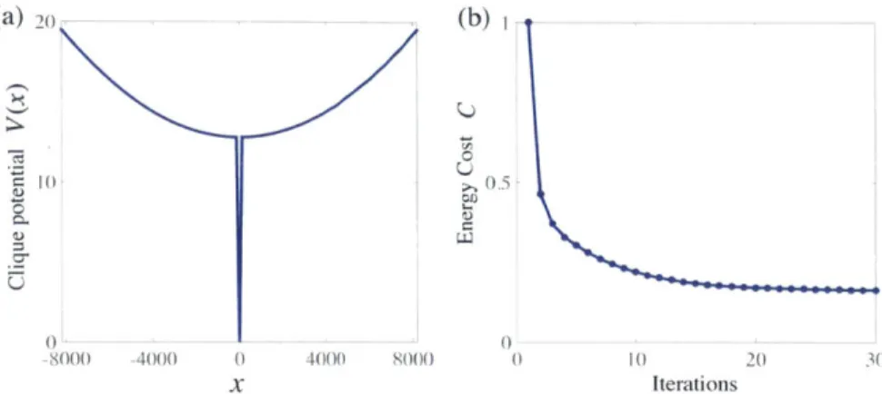
The design of a good potential function V1(x) is crucial in the optimization. Quadratic functions are typically used in energy minimizations, but it is well-known that they tend to smooth the result while doing image restoration. Different from unwrapping in optics,
where signals are mostly smooth, natural images usually contain high frequency features, such as edges. Based on the investigation of [24] on the statistical properties of HDR images under gradient domain representation, we design a piecewise potential function comprised of a linear and a quadratic function to estimate their gradient probability distri-bution:
V(x) = aix
H
0 (2.5)a2x2
+
b Ixj > xowhere we empirically choose a, = 0.1, a2 = 10
5 , and xO
2N-1, as plotted in Fig.
2-5(a). These parameters determine prior smoothness of the latent image, and they are fixed for all our experiments in this paper.
From Eq. (2.4), we would easily find that convex functions satisfy the graph-representable requirement, which means energy drop is guaranteed at each step until convergence. While our designed potential function is able to preserve sharp changes in natural images, it vio-lates the graph-representable requirement. Hence, we put additional constraints to ensure good cuts for each iteration and avoid being trapped in local minimum. We adopt a similar approach as proved in [6]. Whenever Eq. (2.4) is not reached, we set the weight of the edge
(v, v') to zero meaning this elementary graph does not contribute in energy increase in the
s-t cut; whenever energy is minimized, step size 6 is extended to look for lower possible energy, namely we shift to 6 c {0, -} for further iterations, where we empirically choose
= 2.
We show the intermediate and converged results of the unwrapping example in Fig. 2-6. The four linear images in Fig. 2-6(a) illustrate the progressive recovering capability of the graph cuts algorithm, and the disappearance of fringes due to the removal of rollovers could be obviously observed. The final unwrapping result is free of errors compared to ground truth in this test. Fig. 2-6(b) shows the tone-mapped image of the final result. The normalized energy drop at each iteration is plotted in Fig. 2-5(b) which clearly shows good convergence of the algorithm.
(b)
() 2)3
Iterations
Figure 2-5: (a) The piecewise energy function to be minimized for natural HDR images; (b) Energy drop during each iteration for the case in Fig. 2-4(a).
'
TIl
512 0 i12 1024 0 1500
(i)
0 4000 8000 ( 0.5
(h)
Figure 2-6: (a) Intermediate unwrapping solution at each iteration: from left to right {1, 3. 10, 30}. The images are linearly scaled in intensity, where gray bars below tell the corresponding intensity values for each image; (b) Tone-mapped image of the final result.
26
I
4 4I-fl! (I (0 x (a) 'Q000 10()(02.4 Multi-shot HDR fusion
The single modulus image unwrapping can extend the dynamic range greatly, but it is ill-posed after all. When multiple modulus images under different exposures are available, the problem becomes over-determined. We analyze in this section that merging multiple modulo images has great advantages in both dynamic range recovery and preserving details of the scene.
2.4.1
Accurate scene radiance estimation
To record a scene with contrast 65, 000 : 1 (16 stops), theoretically capturing two images with exposure ratio of 256 : 1 using an 8-bit intensity camera is enough. Unfortunately, merely combining these two images will lose too much details since it is always challenging to capture both high dynamic range and detailed scene radiance using an intensity camera. Intuitively, the under-exposed image is "black" in most areas and the over-exposed image is almost "white" everywhere. That's why people usually take more than two captures
(E.g., five images with exposure ratio of 4 x, nine images with exposure ratio of 2 x) for high quality HDR imaging. With a modulo camera, we can achieve the win-win in both very high dynamic range and very detailed scene radiance preservation using as few as two images.
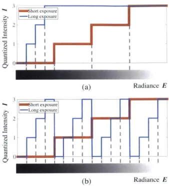
As we focus on sensors with a linear response, observed intensity value is proportional to scene radiance. Here, we borrow the expression from Grossberg and Nayar [25] to use a quantized response function I =
f
(E) to represent the the quantized image intensity valueI corresponding to the scene radiance E. The response function is a piecewise constant function that characterizes the quantization process of a camera. We start with a simple case of two shots by a 2-bit camera for an easy illustration. As shown in Fig. 2-7(a), due to saturation, an intensity camera does not give any radiance discrimination for large radiance during long exposure image capture; for the short exposure image, on the other hand, large quantization steps "flatten" many radiance details.
A modulo camera makes the story totally different. As shown in Fig. 2-7(b), its re-sponse function of the long exposure capture is periodically repeating with a much smaller
quantization step. With this uniform radiance measuring intervals of small steps, the com-plete dynamic range of the scene is sampled equivalently to using a 4-bit linear camera, providing much more measured scene radiance levels than an intensity camera. Although there exists wrapped values while only one long exposure image is used, reconstruction is quite easy with the help of the short exposure image, as we will introduce next.
2.4.2 Multiple modulus images unwrapping
HDR merging from conventional linear images includes weighting and averaging. Weights
are assigned to all pixels in photos of different exposures. In the simplest case, a binary mask is generated for each image to exclude over-exposed and under-exposed pixels. Av-erage is then taken for each pixel on different images to get a linear HDR map. In the masking process, around half of all pixels have zero weights.
The modulus images avoid the annoying over-exposure problem and keep much more useful information. Since the images with longer exposures keep more radiance details but come with wrapped values, while shorter exposure images have less details without wrapped values, so we can simply use images with shorter exposures to unwrap the longer ones.
Assuming we have m modulus images as input, we first sort them according to their
exposure times in an ascending order, and radiance map is initialized to be E(0) = 0. We
start from the shortest exposure image that does not have any rollovers and end up with the longest exposure. When processing each image, the number of rollovers in the new image
k) is calculated from previous radiance map E(-), where the superscript indicates the
image index:
k 2N (2.6)
And then a finer radiance map is updated by combining rollovers k) and the modulus
i.()
from the previous image:
E
k 2
.+ (2.7)noshot eXpOSUIVC - Long exposure (a) Radiance E m Short exposure Long exposure (b) Radiance E
Figure 2-7: Illustration of response function I
f(E)
for short and long exposures. All possible (continuous) radiance levels are shown on the bar below: (a) Intensity camera; (b)Modulo camera.
By this analogy, a final radiance map E(") is achieved with the finest radiance levels. To guarantee that the radiance map can be obtained without wrapped values, the exposure ratio between neighboring images should be < 2^, = {1. 2,3. . m - i}, which is usually satisfied. If rollovers exist in the shortest exposure image, the single image unwrapping method discussed in Sec. 2.3 can be applied first, but here we do not consider this case.
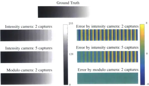
Using a conventional camera, capturing more images is a strategy that helps in reducing these errors, but it affects in a very limited scale. A more intuitive comparison between HDR from intensity images and modulus images is shown in Fig. 2-8. A continuous band (I -D image) whose values linearly range from 0 to 255 is used to represent the complete dynamic range of a scene. We compare the radiance reconstruction by three methods with 4-bit cameras: an intensity camera with 2 captures, an intensity camera with 5 captures and a modulo camera with 2 captures. In the case of 2 captures, exposure difference of 16 times is used; and for the case of 5 captures, their exposures differ by twice for each capture. Left column of Fig. 2-8 shows the reconstructed bands with different methods, and
Ground Truth
Intensity cam er8: 2 captures Error by In tni Cm er: 2 CIpt res Intensity camera: 5 captures Error bv intensitv camera: 5 captures MOdILiO camera: 2 captures Error by modU camera: 2 captures
FigUre 2-8: Comparison between multi-shot HDR using an intensity carnera and a modulo camera. Under multiple exposures. reconstructions with an intensity camera suffers from severe quantization effects in high radiance areas: a modulo camera is able to reconstruct radiance with low errors in all regions.
riaht column is their difference maps with respect to ground truth. We can observe obvious quantization effects in both 2 captures and 5 captures cases for an intensity camera. More captures is an effective strategy in reducing errors in low radiance regions, but does not help for large radiance values, showing its inherent limitation. In contrast, fusion of modulus images gives an almost perfect reconstruction that equally preserves details from low to high radiance levels. The analysis here applies to higher contrast images as well. but due to the difficulty to show images higher than 8-bit in both printed papers and ordinary computer
monitors we omit such an illustration here.
Sampling a large range of radiance values uniformly with a sufficiently small step (equivalent to using a higher bit depth linear camera) is meaningful in many computer vision applications like inverse rendering, photometric shape recovery, etc. However, to reach this goal with a linear intensity camera is not easy [25]. Highly irregular exposure ratios (like {I : 1.003 : 2.985} for three captures), which are extremely difficult to set in common cameras, are required. What is worse, according to [251, taking {2. 3. 4, 5. 6} captures can only reach the dynamic range of {256 : 1. 761 :1. 93 :1. 1269 : 1. 1437 : 1
camera only requires exposure ratios of 2"(M E Z), which are more commonly used se-tups in cameras. To maximize the dynamic range, a simple strategy is to set exposure ratio to maximum, which is 2N. Visible radiance contrast in real life photography normally does
not exceed 10,000,000:1 (within 24 stops), meaning three captures with a modulo camera is sufficient for capturing high quality HDR images. Comparably, three captures with an intensity camera only gives an HDR with limited range, which is a known fact.
2.5
Experiments
2.5.1
Synthetic test
We simulated experiments for both single- and multi-shot HDR. Ground truth images are either obtained from online datasets or taken with a 12-bit Sony NEX camera.
Single-shot HDR
To validate our unwrapping framework, ground truth images are chosen to have maxi-mum contrast ranging from 1024 : 1 (10 stops) to 4096 : 1 (12 stops), while actual con-trasts differ as per example. The 8-bit intensity images are synthesized by truncating the brightness values over 255 to 255, and the 8-bit modulus images are easily simulated by dropping the higher bits (>8) of the ground truth. A tone mapping scheme by adaptive histogram equalization [34] is applied on our results for visualization.
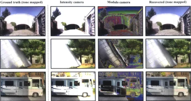
In Fig. 2-9, ground truth, images taken by an intensity camera, images taken by a mod-ulo camera and unwrapped results are shown from left to right. Wrapped regions in the modulus images correspond to saturated regions in the intensity images. Our unwrapping algorithm recovers these wrapped values back to their true values. As shown, images are restored successfully even with large areas of "saturation".
Multi-shot HDR
Then we compare the multi-shot HDR recovery of an intensity camera and a modulo camera. 8-bit ground truth images are chosen to make visualizable evaluation, and 4-bit
images are synthesized as outputs of both cameras.
Fig. 2-10 shows several results from our experiment comparing: ground truth, recon-struction by an intensity camera and a modulo camera with different number of captures. Exposure ratio is {1 : 16} for the case of 2 captures, and {1 : 2 : 4 : 8 : 16} for 5 captures. Close-up views highlight the visible details in the dashed squares. Quantization noise is visible in images from an intensity camera, but not in those from a modulo camera.
2.5.2
Real experiment
Finally our work leverages an existing modulo camera (DFPA) to show the effectiveness of our proposed framework. Details associated with DFPA sensor design and camera pro-totype are introduced in [56, 9, 18]. We acquired 8-bit modulus images at a resolution of
256 x 256.
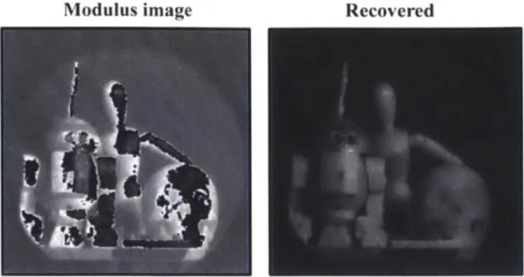
The single-shot modulus image shown in Fig. 2-11 is captured with an exposure time spanning 2000 ms. Our proposed unwrapping algorithm is applied on the modulus image for recovery.
Multi-shot merging experiment is shown in Fig. 2-12. The exposure time for short and long exposure images are 100 ms and 4000 ms, respectively. The short exposure image suffers from a strong quantization effects. After it is merged with the long exposure image, we could visualize the reduced quantization noise in the close-up view.
2.6 Discussion
Our single-image unwrapping algorithm could greatly extend the dynamic range of a mod-ulus image of real world scenes, as we have evaluated in the experiment section. Theo-retically, the dynamic range of recovery is not bounded in a modulus image. However, single-image unwrapping is ill-posed as recoveries are done solely based on local prop-erties of pixel values, making the formulation only come with a smoothness constraint. Therefore, the success of unwrapping is partially dependent on the input data as well. In general, extremely large local contrast in original intensities makes the unwrapping solu-tion more prone to errors, ie., the unwrapping operasolu-tion is ideal for continuous, smooth
Groni d tiruth (tonie nipped) Inteusity camera MIodttlo C1ittrrra
hi-i
_
_J
Ri. c-uc. I (toie mai ppedl)
it~
Figure 2-9: Single-shot HDR recovery. Regions in the modulus images with wrapped values correspond to saturated regions in the
row is courtesy of Raanan Fattal.
intensity images. Radiance data of the first
Ground titith
Riir
Intensity camera: c aptures
In
p
NU
IodiiIo canier: 2 capuires
Figure 2-10: Multi-shot HDR fusion. Close-up views highlight the visible details in dashed squares. Quantization noise is visible in images from an intensity camera, but not in those from a modulo camera. Best viewed electronically.
.2
Inte"SiIA Camera: 2 Captilres
1:71
Modulus image Recovered
Figure 2-11: Real experiment: single shot. The modulus image is unwrapped to become an HDR image.
HDR reconstruction, but it will fail in cases like impulse functions. Natural images are cases just sitting between them. Under the representation of modulus images, when fringes are dense enough to cause spatial aliasing, they are hard to be solved correctly. Fig. 2-13 is an example where unwrapping fails in the region of a super bright sun, as marked by the blue dashed lines. In this case, two captures are required to help recover the radiance map. The quantitative limit of unwrapping algorithm is an interesting open problem.
In multi-shot HDR fusion, if we only care about capturing the finest radiance levels, but not uniform sampling like a linear camera, choosing integer exposure ratios is not optimal due to overlaps of quantization levels. Therefore, non-integer exposure ratios are necessary to achieve even finer radiance recovery, but seeking the best non-integer exposure values is left as future work.
In the real experiment, as our camera prototype is still at its initial stage, it suffers from limitations like low sensor filling factor and low quantum efficiency, which result in relatively long exposure time and strong noise. As noise is more obvious in the least significant bits, it will degrade the recovery performance. To visualize the possible failures caused by noise, a longer exposure of 8000 ims modulo image is intentionally captured, as shown in Fig. 2-14. The number of wraps and noise level are both much higher than the same scene in Fig. 2-1l. Artifacts in the unwrapped result are caused by both factors.
Short exposure Long exposure
i
( Io.s-up comlparison
-I
Figure 2- 12: Real experiment: multiple shots. Brightness is linearly adjusted for visualiza-tion. After merging the short and long exposure, the details of radiance values are better preserved.
Ground truth
Recovered: 1 capture
2 captures
Fioure 2- 13: Failure case - synthetic data: when the local dynamic range of ground truth is extremely huge (the region in the sun), our single modulo image unwrapping method may fail, multiple-shot recovery is required. Radiance map is courtesy of Jack Tumblin.
Modulus input
Figure 2-14: Failure case - real data: strong noise in this case is created by extending the exposure time.
Chapter 3
Sub-Pixel Layout for Super-Resolution
with Images in the Octic Group
High-resolution photography is a common goal for commercial cameras on the market today. The resolution of an image is fundamentally determined by the interval between sensor pixels. To overcome this limit, super-resolution (SR) technique can be performed by taking multiple frames with sub-pixel displacements of the same scene. However, even with a large number of images under sufficiently small-step displacements, the performance of SR algorithms can hardly extend beyond small magnification factors of 2 to 4 [3, 35],
partially due to the challenges associated with proper alignment of local patches with finer translations [61].
We note here that the geometry of the pixels usually has been assumed to lie on a rectangular grid. This geometric restriction limits the information captured for each sub-pixel shift, because repeating the observations at integer sub-pixel intervals are redundant. An aperiodic pixel layout [4] or a random disturbance to pixel shapes [50] could break the the-oretical bottleneck of conventional SR by effectively avoiding the redundancy due to trans-lational symmetry. These structures provide greater variation with sub-pixel displacements to result in more independent equations for recovering high-frequency spatial information. In this study, we' explore the properties of non-conventional pixel layouts and shapes. Some existing CCDs contain sub-pixels of different shapes and spatial locations within one
pixel. Two examples are shown in the bottom row of Fig. 3-1. The Orthogonal-Transfer Charge-Coupled Device (OTCCD) sensor [10] has four sub-pixels2
, and the Super CCD [20] has two3. These sub-pixels naturally increase the spatial sampling rate. Instead of relying on sub-pixel displacements, however, we focus on forming multiple images via transformations in the octic group, i.e. all symmetries of a square. We assume the pixel shape is square, so that each element in the octic group corresponds to one pose of a pixel. The sub-pixel layout varies with different poses of a pixel, and depends on the layout's symmetry. For example, the OTCCD can form 8 different sub-pixel layouts (through four 90' rotations and their reflections), but the Super CCD has left-right symmetry and there-fore shows only 4 different layouts. By combining multiple images recorded with different poses, a super-resolved image with higher resolution can be obtained. The intuition here is that more sub-pixels with asymmetric layouts can construct a higher resolution image. We discuss here the exact relationship between sub-pixel layout (including the number and distribution of sub-pixels) in the octic group and the magnification factor.
The key contributions of this work are summarized as below:
" A new framework that provides a novel view to the SR problem by using an asymmet-ric sub-pixel layout to form multiple images in the octic group. Instead of focusing on a particular layout, we investigate the theoretical bound of SR performance w.r.t. the number and distribution of sub-pixels (Sec. 3.2.2).
" Based on the theoretical analysis, a sub-pixel layout selection algorithm is proposed to choose good layouts for well-posed and effective SR (Sec. 3.2.3).
* We propose a simple yet effective SR reconstruction algorithm (Sec. 3.3) and validate our theory and algorithm using both synthetic and real data (Sec. 3.4).
2
The OTCCD actually consists four phases in one pixel. Photon charges are integrated separately in each phase and can be shifted between the phases. Here we interpret the four "phases" as four "sub-pixels".
3
1f we treat the gap among sub-pixels as another sub-pixel that does not record photon charges, the number of sub-pixels could be five for the OTCCD and three for the Super CCD.
Conventional CCD 0 TCCD images rotated by 0, 90, 180, and 270 degrees SR result
'1
L
f2014
An I CC 0 pixel (with 4 sub-pixels) in thle octiC group A super CCD pixel (with 2 sub-pixels) in the uctiC group
Figure 3-1: Existing CCD sensors with non-conventional sub-pixel layouts (bottom row).
By transforming the image plane, their images in the octic group show different sub-pixel layouts, which can be combined for significant resolution enhancement (top row). The OTCCD images under 4 rotations can perform 4 x SR. Comparing the OTCCD with the Super CCD, it can be seen that sub-pixels with an asymmetric layout produce more varia-tion in their images in the octic group.
3.1
Related Works
Our approach belongs to the category of reconstruction-based SR with multiple images. Single-image based SR algorithms such as learning-based methods (e.g., [19]) are beyond the scope of this study. We refer the readers to survey papers (e.g., [46]) for a discussion of various categories of SR algorithms.
For regular pixel layouts and shapes, there are various SR reconstruction methods for images with sub-pixel displacements. Popular approaches include iterative back projection (IBP) [30], maximum a posteriori and regularized maximum likelihood 114] and sparse representation 159]. These reconstruction techniques Focus on solving the ill-posed inverse problem with a conventional sensor and setup.
In contrast, this thesis studies asymmetric sub-pixel layouts and is therefore similar to former techniques using non-conventional pixel layouts [4] and pixel shapes [501. The pre-vious work used a Penrose pixel layout, which never repeats itself, on an infinite plane. The latter work implemented random pixel shapes by spraying fine-grained black powder on the CCD. Both methods focus on one type of layout or shape and use multiple images
1/4 1/8 114 1/8 1/2 0 1 0 0 0
1/16 1/8 1/8 1/4 0 1/2 1/2 0 0 1 0 0.37
4 1 3 64 3,16 10 1, _' 1 2 0u 0 0 1 10 0 3/4 1/4
7 W1
0 0.300(a) (b) (C) (d) (M)
Figure 3-2: Different sub-pixel layouts and their HR-to-LR mapping matrices P, with magnification factor M = 2. (a) Conventional SR: LR pixels with double the size as HR pixels undergo a sub-pixel displacement; (b)-(e): examples of different sub-pixel layouts. Different color-shaded areas (RGBYW here) represent different sub-pixels, and the white area within one pixel is to simulate a gap that does not record photon charges.
with sub-pixel displacements. Our work is different from them in two ways: 1) We trans-form the image plane to trans-form multiple images in the octic group; 2) We propose a general theory and categorize good sub-pixel layouts for deeper understanding of SR performance
with non-conventional pixels.
3.2
Good Sub-pixel Layout for Super-Resolution
3.2.1
Single image case
Similar to Penrose tiling [41, we ignore optical deblurring and assume that it can be applied after sub-pixel sampling. Thus, in the discrete domain, reconstruction-based SR can be represented as a linear system as
L =PH + E. (3.1)
where H includes all pixels of a high resolution (HR) image in a column vector, L concate-nates column vectors formed by all low resolution (LR) images, P is the matrix that maps HR to LR images, and E is the per-pixel noise.
In the ideal case when noise can be ignored, to double the resolution (2x SR), we need at least 4 LR images with exactly half-pixel shifts to produce a full reconstruction
(the inverse problem is well-posed). In general, the displacements of LR images can be arbitrary, and they determine the values in P. An example of P is shown in Fig. 3-2(a). The HR grid is drawn with dashed lines, and the shaded squares with different colors represent LR pixels from different images. In this example, P is evaluated for the 2 x 2 area indicated by the bold black square (values out of this area are not shown). Each row of P corresponds to one displaced-LR pixel (shaded area with the same color), and the element in each row is calculated for all HR pixels (bold black square in Fig. 3-2) as the area ratio of overlapping regions to the LR pixel size. The analysis of P plays a key role in understanding the performance of SR.
Similar to sub-pixel displacement with multiples images, the increase in spatial sam-pling can also be implemented by splitting one LR pixel into smaller sub-pixels with a single image. The most straightforward example for the 2x SR is splitting one LR pixel into 4 square regions, as shown in Fig. 3-2(c). In such a case, P is an identity matrix. By treating each sub-pixel as a displaced LR pixel, we can build P for sub-pixel.layouts in Fig. 3-2(b), (d), and (e) in a similar way as Fig. 3-2(a). Note the layout in (b) has rank(P) = 2, so it cannot produce 2 x SR. The layouts in (d) and (e) have rank(P) = 4, so they can achieve 2 x SR. For easy analysis, we assume the sub-pixels completely cover one LR pixel, so the layouts in Fig. 3-2(d) and (e) actually have 5 sub-pixels. We treat the gap among sub-pixels as a dumb sub-pixel that does not record photon charges; therefore, strictly speaking, P for layouts (d) and (e) should have an all-zero row, which is omitted in the figure.
In general, the size of P equals to r x M 2
, where r is the number of sub-pixels, and M as the magnification factor. It is easy to infer that for a single pixel with r sub-pixels, to achieve M x SR, the sufficient condition for full reconstruction is when r > M2. Because
the full reconstruction is achieved when rank(P) = M 2
and P has the size of r x M2,
rank(P) < M2holds if r < M2
0 0 0 14 '14 1401 0 0 14 0 0 0) (0 "1 0 0 0 4 0 0 0 14 1A 4 0 0 1
e R?
10 ) 0
Figure 3-3: Sub-pixel layouts with r =5 (the gap among sub-pixels is a dumb sub-pixel) in a sub-group of the octic group T?1. c . 1.H.
TH}.
These layouts could build a P withrank(P) =16. Four images captured with such sub-pixel layouts can be used to perform 4x SR.
3.2.2
Multiple images in the octic group
Enhancing the resolution by only using sub-pixels in one image has limited performance (requires r > A42). Further, in practice, increasing the sub-pixel number cannot continue indefinitely, due to manufacturing limitations and the proportionality between pixel size and light collection efficiency (emphi.e., signal-to-noise ratio (SNR) decreases with pixel size). Combining different sub-pixel layouts for one pixel can further enhance the resolu-tion, but physically modifying the layout in a fabricated sensor is cost prohibitive. Instead, we observe that simple operations on the image plane can serve to change the sub-pixel layouts, if we make multiple images to form the octic group.
Octic group
In group theory, a square belongs to the octic group, which is the 4-th order dihedral group. This group contains 8 components that keep all symmetric properties of a square, denoted
as
Q C. R1.R 5 R . 51 su, . v?: (3.2.)&
where c represents the original pose; H1, , and Htj represent 90', 180' and 2700 rotations
of the original pose; and S, , Hl?, Su, and 5/: represent the reflections (horizontal or vertical mirror flipping) to the first 1 elements, respectively. These 8 poses can transform into each other according to the multiplication table of the octic group.