Hedging of covered options with linear market impact and gamma constraint

HAL Id: hal-01611790

https://hal.archives-ouvertes.fr/hal-01611790

Submitted on 6 Oct 2017

HAL is a multi-disciplinary open access

archive for the deposit and dissemination of sci-entific research documents, whether they are pub-lished or not. The documents may come from

L’archive ouverte pluridisciplinaire HAL, est destinée au dépôt et à la diffusion de documents scientifiques de niveau recherche, publiés ou non, émanant des établissements d’enseignement et de

Hedging of covered options with linear market impact

and gamma constraint

Bruno Bouchard, G. Loeper, Y. Zou

To cite this version:

Bruno Bouchard, G. Loeper, Y. Zou. Hedging of covered options with linear market impact and gamma constraint. SIAM Journal on Control and Optimization, Society for Industrial and Applied Mathematics, 2017, 55 (5), pp.3319-3348. �hal-01611790�

Hedging of covered options with linear market

impact and gamma constraint

B. Bouchard

_{, G. Loeper}

_{and Y. Zou}

January 6, 2016

Abstract

Within a financial model with linear price impact, we study the problem of hedging a covered European option under gamma con-straint. Using stochastic target and partial differential equation smooth-ing techniques, we prove that the super-replication price is the viscosity solution of a fully non-linear parabolic equation. As a by-product, we show how "-optimal strategies can be constructed. Finally, a numerical resolution scheme is proposed.

Keywords: Hedging, Price impact, Stochastic target. AMS 2010 Subject Classification: 91G20; 93E20; 49L20

Introduction

Inspired by [1, 18], the authors in [4] considered a financial market with permanent price impact, in which the impact function behaves as a linear function (around the origin) in the number of bought stocks. This class of models is dedicated to the pricing and hedging of derivatives in situations where the notional of the product hedged is such that the delta-hedging is non-negligible compared to the average daily volume traded on the underlying asset. Hence, the delta-hedging strategy will

⇤_{Paris-Dauphine University, PSL Research University, CEREMADE, UMR 7534, 75775}

Paris cedex 16, France.

†_{Research supported by ANR Liquirisk}

have an impact on the price dynamics, and will also incur liquidity costs. The linear impact models studied in [1, 4, 18] incorporate both the effects into the pricing and hedging of the derivative, while maintaining the completeness of the market (up to a certain extent) and eventually leading to exact replication strategies. As in perfect market models, this approach can provide an approximation of the real market conditions that can be used by practitioners to help them in the design of a suitable hedge in a systematic way, without having to rely on an ad hoc risk criterion.

In [4], the authors considered the hedging of a cash-settled European option: at inception the option seller has to build the initial delta-hedge, and conversely at maturity the hedge must be liquidated to settle the final claim in cash. It is shown therein that the price function of the optimal super-replicating strategy no longer solves a linear parabolic equation, as in the classical case, rather a quasi-linear one. Moreover, the hedging strategy consists in following a modified delta-hedging rule where the delta is computed at the “unperturbed” value of the underlying, i.e., the one the underlying would have if the trader’s position were liquidated immediately. The approach and the results obtained in [4] thus differ substantially from [1, 18]. Indeed, while in [1, 18] the impact model considered is the same, the control problem is different in the sense that it is applied to the hedging of covered options. This refers to situations where the buyer of the option delivers at inception the required initial delta position, and accepts a mix of stocks (at their current market price) and cash as payment of the final claim, which eliminates the cost incurred by the initial and final hedge. Quite surprisingly, this is not a genuine approximation of the problem studied in [4]. The question of the initial and final hedge is fundamental, to the point that the structure of the pricing question is completely different: in [4] the equation is quasi-linear, while it is fully non-linear in [1, 18].

As opposed to [4], authors in [1, 18] use a verification argument to build an exact replication strategy. Due to the special form of the non-linearity, the equation is ill-posed when the solution does not satisfy a gamma-type constraint. The aim of the current paper is to provide a direct characterization via stochastic target techniques, and to incorporate right from the beginning a gamma constraint on the hedging strategy.

The super-solution property can be proved by (essentially) following the argu-ments of [8]. The sub-solution characterization is much more difficult to obtain. Actually, we could not prove the required geometric dynamic programming princi-ple, unlike [8], because of the strong interaction between the hedging strategy and the underlying price process due to the market impact. Instead, we use the smooth-ing technique developed in [5]. We construct a sequence of smooth super-solutions which, by a verification argument, provide upper-bounds for the super-hedging

price. As they converge to a solution of the targeted pricing equation, a compar-ison principle argument implies that their limit is the super-hedging price. As a by-product, this construction provides explicit "-optimal hedging strategies. We also provide a comparison principle and a numerical resolution scheme. For sim-plicity, we first consider a model that has only permanent price impact, we explain in Section 3 why adding a resilience effect does not affect our analysis. Note that this is because the resilience effect we consider here has no quadratic variation, as opposed to [1], in which the resilience can destroy the parabolicity of the equation, and renders the exact replication non optimal.

We close this introduction by pointing out some related references. [6] incor-porates liquidity costs but no price impact, the price curve is not affected by the trading strategy. It can be modified by adding restrictions on admissible strate-gies as in [7] and [24]. This leads to a modified pricing equation, which exhibits a quadratic term in the second order derivative of the solution, and renders the pricing equation fully non-linear, and even not unconditionally parabolic. Other articles focus on the derivation of the price dynamics through clearing condition, see e.g., [12], [22], [21] in which the supply and demand curves arise from “reference” and “program” traders (i.e., option hedgers); leading to a modified price dynamics, but without taking into account the liquidity costs, see also [17]. Finally, the series of papers [23], [8], [24] addresses the liquidity issue indirectly by imposing bounds on the “gamma” of admissible trading strategies, no liquidity cost or price impact are modeled explicitly.

General notations. Throughout this paper, ⌦ is the canonical space of contin-uous functions on R+ starting at 0, P is the Wiener measure, W is the canonical

process, and F = (Ft)t 0is the augmentation of its raw filtration F = (Ft)t 0. All

random variables are defined on (⌦, F1,P). We denote by |x| the Euclidean norm

of x 2 Rn_{, the integer n 1 is given by the context. Unless otherwise specified,}

inequalities involving random variables are taken in the P a.s. sense. We use the convention x/0 = sign(x) ⇥ 1 with sign(0) = +.

1 Model and hedging problem

This section is dedicated to the derivation of the dynamics and the description of the gamma constraint. We also explain in detail how the pricing equation can be obtained and state our main result.

1.1 Impact rule and discrete time trading dynamics

We consider the framework studied in [4]. Namely, the impact of a strategy on the price process is modeled by an impact function f: the price variation due to buying a (infinitesimal) number 2 R of shares is f(x), given that the price of the asset is x before the trade. The cost of buying the additional units is

x +1 2 2_{f (x) =} Z 0 1 (x + ◆f (x))d◆, in which _Z 0 1 (x + ◆f (x))d◆

can be interpreted as the average cost for each additional unit.

Between two trading instances ⌧1, ⌧2 with ⌧1  ⌧2, the dynamics of the stock is

given by the strong solution of the stochastic differential equation dXt= µ(Xt)dt + (Xt)dWt.

Throughout this paper, we assume that f _{2 C}2

b and inf f > 0,

(µ, ) is Lipschitz and bounded, inf > 0. (1.1)

As in [4], the number of shares the trader would like to hold is given by a continuous Itô process Y of the form

Y = Y0+ Z _· 0 bsds + Z _· 0 asdWs. (1.2)

We say1 _{that (a, b) belongs to A}

k if (a, b) is continuous, F-adapted,

a = a0+ Z _· 0 s ds + Z _· 0 ↵sdWs

where (↵, ) is continuous, F-adapted, and ⇣ := (a, b, ↵, ) is essentially bounded by k and such that

E⇥sup |⇣s0 ⇣_s|, t  s  s0  s +  T |F_t⇤ k

for all 0   1 and t 2 [0, T ].

1_{In [4], (a, b) is only required to be progressively measurable and essentially bounded.}

We then define

A := [kAk.

To derive the continuous time dynamics, we first consider a discrete time setting and then pass to the limit. In the discrete time setting, the position is re-balanced only at times

tn_i := iT /n, i = 0, . . . , n, n 1. In other words, the trader keeps the position Ytn

i in stocks over each time interval

[tn_i, tn_i+1). Hence, his position in stocks at t is

Y_tn:= n 1 X i=0 Ytn i1{tnit<tni+1}+ YT1{t=T }, (1.3)

and the number of shares purchased at tn i+1 is n tn i+1:= Yt n i+1 Ytni.

Given our impact rule, the corresponding dynamics for the stock price process is Xn= X0+ Z _· 0 µ(X_sn)ds + Z _· 0 (X_sn)dWs+ n X i=1 1_[tn i,T ] n tn if (X n tn i ), (1.4) in which X0 is a constant.

The portfolio process is described as the sum Vn _{of the amount of cash held}

and the potential wealth Yn_Xn _{associated to the position in stocks:}

Vn=cash position + YnXn.

It does not correspond to the liquidation value of the portfolio, except when Yn_{= 0.}

This is due to the fact that the liquidation of Yn _{stocks does not generate a gain}

equal to Yn_Xn_{, because of the price impact. However, one can infer the exact}

composition in cash and stocks of the portfolio from the knowledge of the couple (Vn_{, Y}n_).

Throughout this paper, we assume that the risk-free interest rate is zero (for ease of notations). Then,

Vn= V0+ Z _· 0 Y_sndX_sn+ n X i=1 1_[tn i,T ] 1 2( n tn i) 2_{f (X}n tn i ). (1.5)

This wealth equation is derived as in [4] following elementary calculations. The last term of the right-hand side comes from the fact that, at time tn

i, tnn

i shares are

bought at the average execution price Xn tn i + 1 2 ntn if (X n tn

i ), and the stock’s price

ends at Xn tn i + n tn if (X n tn

i ), whence the additional profit term. However, one can

Remark 1.1. Note that in this work we restrict ourselves to a permanent price im-pact, no resilience effect is modeled. We shall explain in Section 3 below why taking resilience into account does not affect our analysis. See in particular Proposition 3.1.

1.2 Continuous time trading dynamics

The continuous time trading dynamics is obtained by passing to the limit n ! 1, i.e., by considering strategies with increasing frequency of rebalancement.

Proposition 1.2. [4, Proposition 1] Let Z := (X, Y, V ) where Y is defined as in (1.2) for some (a, b) 2 A , and (X, V ) solves

X = X0+ Z _· 0 (Xs)dWs+ Z _· 0 f (Xs)dYs+ Z _· 0 (µ(Xs) + as( f0)(Xs))ds = X0+ Z _· 0 as X(Xs)dWs+ Z _· 0 µas,bs X (Xs)ds (1.6) with as X := ( + asf ) , µ as,bs X := (µ+bsf + as f0), and V = V0+ Z _· 0 YsdXs+ 1 2 Z _· 0 a2_sf (Xs)ds. (1.7)

Let Zn _{:= (X}n_{, Y}n_{, V}n_{) be defined as in (1.4)-(1.3)-(1.5). Then, there exists a}

constant C > 0 such that sup

[0,T ]E

⇥

|Zn Z_|2⇤_{ Cn} 1

for all n 1.

For the rest of the paper, we shall therefore consider (1.7)-(1.6) for the dynamics of the portfolio and price processes.

Remark 1.3. As explained in [4], the previous analysis could be extended to a non-linear impact rule in the size of the order. To this end, we note that the continuous time trading dynamics described above would be the same for a more general impact rule 7! F (x, ) whenever it satisfies F (x, 0)= @2 _{F (x, 0) = 0 and}

@ F (x, 0) = f (x). For our analysis, we only need to consider the value and the slope of the impact function at the origin.

1.3 Hedging equation and gamma constraint

Given = (y, a, b)_{2 R ⇥ A and (t, x, v) 2 [0, T ] ⇥ R ⇥ R, we now write (X}t,x, _,

Yt, , Vt,x,v, ) for the solution of (1.6)-(1.2)-(1.7) associated to the control (a, b) with time-t initial condition (x, y, v).

In this paper, we consider covered options, in the sense that the trader is given at the initial time t the number of shares Yt = y required to launch his hedging

strategy and can pay the option’s payoff at T in cash and stocks (evaluated at their time-T value). Therefore, he does not exert any immediate impact at time t nor T due to the initial building or final liquidation of his position in stocks. Recalling that V stands for the sum of the position in cash and the number of held shares multiplied by their price, the super-hedging price at time t of the option with payoff g(X_Tt,x, ) is defined as

v(t, x) := inf_{{v = c + yx : (c, y) 2 R}2 s.t. G(t, x, v, y) 6= ;},

in which G(t, x, v, y) is the set of elements (a, b) 2 A such that := (y, a, b) satisfies

V_Tt,x,v, g(X_Tt,x, ).

In order to understand what the associated partial differential equation is, let us first rewrite the dynamics of Y in terms of X:

dY_tt, = at Y (X t,x, t )dXtt,x, + µaYt,bt(X t,x, t )dt with a Y := a + f a and µ a,b Y := b Yaµa,bX . (1.8)

Assuming that the hedging strategy consists in tracking the super-hedging price, as in classical complete market models, then one should have Vt,x,v, _{= v(·, X}t,x, _).

If v is smooth, recalling (1.6)-(1.7) and applying Itô’s lemma twice implies

Yt, = @xv(·, Xt,x, ) , Ya(Xt,x, ) = @xx2 v(·, Xt,x, ), (1.9) and 1 2a 2_{f (X}t,x, _{) = @} tv(·, Xt,x, ) + 1 2( a X)2(Xt,x, )@xx2 v(·, Xt,x, ). (1.10)

Then, the right-hand side of (1.9) combined with the definition of a

Y leads to a = @ 2 xxv(·, Xt,x, ) 1 f @2 xxv(·, Xt,x, ) , a X = _{1 f @2} xxv(·, Xt,x, ) ,

and (1.10) simplifies to  @tv 1 2 2 (1 f @2 xxv) @_xx2 v (_{·, X}t,x, ) = 0 on [t, T ). (1.11) This is precisely the pricing equation obtained in [1, 18].

Equation (1.11) needs to be considered with some precautions due to the sin-gularity at f@2

xxv = 1. Hence, one needs to enforce that 1 f@xx2 vdoes not change

sign. We choose to restrict the solutions to satisfy 1 f@2

xxv > 0, since having the

opposite inequality would imply that a does not have the same sign as @2 xxv, so

that, having sold a convex payoff, one would sell when the stock goes up and buy when it goes down, a very counter-intuitive fact.

In the following, we impose that the constraint

k Ya(Xt,x, ) ¯(Xt,x, ) , on [t, T ] P a.e., (1.12)

should hold for some k 0, in which ¯ is a bounded continuous map satisfying

◆_{ ¯  1/f} ◆, for some ◆ > 0. (1.13)

We denote by Ak,¯(t, x) the collection of elements (a, b) 2 Ak such that (1.12)

holds and define

A¯(t, x) :=[k 0Ak,¯(t, x).

Then, the equation (1.11) has to be modified to take this gamma constraint into account, leading naturally to

F [v¯] := min ⇢ @tv¯ 1 2 2 1 f @2 xxv¯ @2_xxv¯ , ¯ @xx2 v¯ = 0 on [0, T ) ⇥ R, (1.14) in which v¯ is defined as v but with

G¯(t, x, v, y) :=G(t, x, v, y) \ A¯(t, x)

in place of G(t, x, v, y). More precisely,

v¯(t, x) := inf{v = c + yx : (c, y) 2 R2 s.t. G¯(t, x, v, y)6= ;}. (1.15)

As for the T -boundary condition, we know that v¯(T,·) = g by definition.

However, as usual, the constraint on the gamma in (1.14) should propagate up to the boundary and g has to be replaced by its face-lifted version ˆg, defined as the smallest function above g that is a viscosity super-solution of the equation

¯ @2

xx' 0. It is obtained by considering any twice continuously differentiable

function ¯ such that @2

xx¯ = ¯, and then setting

ˆ

g := (g ¯)conc+ ¯,

in which the superscript conc means concave envelope, cf. [23, Lemma 3.1].2 _Hence,

we expect that

v¯(T ,·) = ˆg on R.

From now on, we assume that ˆ

g is uniformly continuous,

g is lower-semicontinuous, g is bounded and g+ has linear growth. (1.16) We are now in a position to state our main result. From now on

v¯(T, x) stands for lim

(t0, x0)! (T, x) t0< T

v¯(t0, x0)

whenever it is well defined.

Theorem 1.4. The value function v¯ is continuous with linear growth. Moreover,

v¯ is the unique viscosity solution with linear growth of

F [']1[0,T )+ (' g)1ˆ {T }= 0 on [0, T ] ⇥ R. (1.17)

We conclude this section with additional remarks.

Remark 1.5. Note that ˆg can be uniformly continuous without g being continuous. Take for instance g(x) = 1{x K} with K 2 R, and consider the case where ¯ > 0

is a constant. Then, ˆg(x) = [1{x xo}

¯

2(x xo)2]^ 1 with xo := K (2/¯)

1 2.

Remark 1.6. The map ˆg inherits the linear growth of g. Indeed, let c0, c1 0 be

constants such that |g(x)|  w(x) := c0+ c1|x|. Since ˆg g by construction, we

have ˆg  w. On the other hand, since ¯ ◆ > 0, by (1.13), it follows from the arguments in [23, Lemma 3.1] that ˆg  (w ˜)conc_{+ ˜, in which ˜(x) = ◆x}2_/2.

Now, one can easily check by direct computations that

(w ˜)conc= (w ˜)(xo)1[ xo,xo]+ (w ˜)1[ xo,xo]c

with xo:= c1/◆. Hence, (w ˜)conc+ ˜ has the same linear growth as w.

Remark 1.7. As will appear in the rest of our analysis, one could very well in-troduce a time dependence in the impact function f and in ¯. Another interesting question studied by the second author in [18] and [19] concerns the smoothness of the solution and how the constraint on @2

xxv gets naturally enforced by the fast

diffusion arising when 1 f@2

xxv is close to 0.

Remark 1.8 (Existence of a smooth solution to the original partial differential equation). When the pricing equation (1.17) admits smooth solutions (cf. [18] and [19]) that allow to use the verification theorem, then one can construct exact replica-tion strategies from the classical solureplica-tion. By the comparison principle of Theorem 2.11 below, this shows that the value function is the classical solution of the pricing equation, and that the optimal strategy exists and is an exact replication strategy of the option with payoff function ˆg. We will explain in Remark 2.18 below how almost optimal super-hedging strategies can be constructed explicitly even when no smooth solution exists.

Remark 1.9 (Monotonicity in the impact function). Note that the map 2 R 7!

2_(x)M

1 M is non-decreasing on { : M < 1}, for all (t, x, M) 2 [0, T ] ⇥ R ⇥ R. Let

us now write v¯ as vf¯ to emphasize its dependence on f, and consider another

impact function ˜f satisfying the same requirements as f. We denote by vf_¯˜ the corresponding super-hedging price. Then, the above considerations combined with Theorem 1.4 and the comparison principle of Theorem 2.11 below imply that vf˜

¯

vf_¯ whenever ˜f f on R. The same implies that vf_¯ v in which v solves the heat-type equation @t' 1 2 2_@2 xx' = 0 on [0, T ) ⇥ R,

with terminal condition '(T, ·) = g (recall that ˆg g). See Section 4.2 for a numerical illustration of this fact.

2 Viscosity solution characterization

In this section, we provide the proof of Theorem 1.4. Our strategy is the following. 1. First, we adapt the partial differential equation smoothing technique used

in [5] to provide a smooth supersolutions ¯v✏,K,

¯ of (1.17) on [ , T ] ⇥ R, with

✏ > 0, from which super-hedging strategies can be constructed by a standard verification argument. In particular, ¯v✏,K,

¯ v¯ on [ , T ]⇥R. Moreover, this

sequence has a uniform linear growth and converges to a viscosity solution ¯

2. Second, we construct a lower bound v¯ for v¯ that is a supersolution of

(1.17). It is obtained by considering a weak formulation of the super-hedging problem and following the arguments of [8, Section 5] based on one side of the geometric dynamic programming principle, see Section 2.2. It is shown that this function has linear growth as well.

3. We can then conclude by using the above and the comparison principle for (1.17) of Theorem 2.11 below: v¯ ¯v¯ but v¯  v¯  ¯v¯ so that v¯ = ¯v¯ =

v_¯ and v¯ is a viscosity solution of (1.17), and has linear growth.

4. Our comparison principle, Theorem 2.11 below, allows us to conclude that v¯ is the unique solution of (1.17) with linear growth.

As already mentioned in the introduction, unlike [8], we could not prove the required geometric dynamic programming principle that should directly lead to a subsolution property (thus avoiding to use the smoothing technique mentioned in 1. above). This is due to the strong interaction between the hedging strategy and the underlying price process through the market impact. Such a feedback effect is not present in [8].

2.1 A sequence of smooth supersolutions

We first construct a sequence of smooth supersolutions ¯v✏,K,

¯ of (1.17) which

ap-pears to be an upper bound for the super-hedging price v¯, by a simple verification

argument. For this, we adapt the methodology introduced in [5]: we first construct a viscosity solution of a version of (1.17) with shaken coefficients (in the terminol-ogy of [15]) and then smooth it out with a kernel. The main difficulty here is that our terminal condition ˆg is unbounded, unlike [5]. This requires additional non trivial technical developments.

2.1.1 Construction of a solution for the operator with shaken co-efficients

We start with the construction of the operator with shaken coefficients. Given ✏ > 0 and a (uniformly) strictly positive continuous map  with linear growth, that will be defined later on, let us introduce a family of perturbations of the operator appearing in (1.17): F_✏(t, x, q, M ) := min x0_2D✏ (x) min ⇢ q 2_(x0_)M 2(1 f (x0_{)M )}, ¯(x0) M ,

where

D_✏(x) :=_{x0 _{2 R : (x} x0)/(x0)_{2 [ ✏, ✏]}.} (2.1) For ease of notation, we set

F_✏['](t, x) := F_✏(t, x, @t'(t, x), @xx2 '(t, x)),

whenever ' is smooth.

Remark 2.1. For later use, note that the map M 2 ( 1, ¯(x)] 7! 2(x)M 2(1 f (x)M )

is non-decreasing and convex, for each x 2 R, recall (1.13). Hence, (q, M) 2 R ⇥ ( 1, ¯(x)] 7! F✏

(·, q, M) is concave and non-increasing in M, for all ✏ 0.

This is fundamental for our smoothing approach to go through.

We also modify the original terminal condition ˆg by using an approximating sequence whose elements are affine for large values of |x|.

Lemma 2.2. For all K > 0 there exists a uniformly continuous map ˆgK and

xK K such that

• ˆgK is affine on [xK,1) and on ( 1, xK]

• ˆgK = ˆg on [ K, K]

• ˆgK gˆ

• ˆgK ¯ is concave for any C2 function ¯ satisfying @xx2 ¯ = ¯.

Moreover, (ˆgK)K>0is uniformly bounded by a map with linear growth and converges

to ˆg uniformly on compact sets.

Proof. Fix a C2_{function ¯ satisfying @}2

xx¯ = ¯. By definition, ˆg ¯ is concave.

Let us consider an element +_{(resp. ) of its super-differential at K (resp. K).}

Set

ˆ

g_K(x) :=ˆg(x)1_{[ K,K]}(x)

+⇥g(K) + (ˆ ++ @x¯ (K))(x K)⇤1(K,1)(x)

+⇥g( K) + (ˆ + @x¯ ( K))(x + K)⇤1( 1, K)(x).

Consider now another C2 _{function ¯ satisfying @}2

xx¯ = ¯. Since ¯ and ¯ differ

only by an affine map, the concavity of ˆg_K ¯ is equivalent to that of ˆg_K ¯ . The concavity of the latter follows from the definition of ˆgK, as the superdiffential

therefore ˆg_K gˆ. We finally define ˆgK by

ˆ

gK = min{ˆgK, (2c0+ c1| · | ¯ )conc+ ¯ }, (2.2)

with c0 > 0 and c1 0such that

c0 ˆg(x)  c0+ c1|x|, x 2 R,

recall Remark 1.6. The function ˆgK has the same linear growth as 2c0+ c1| · |, by

the same reasoning as in Remark 1.6. Since 2c0 > c0, ˆgK = ˆgK = ˆg on [ K, K].

Furthermore, as the minimum of two concave functions is concave, so is ˆgK ¯ for

any C2 _{function ¯ satisfying @}2

xx¯ = ¯. The other assertions are immediate. ⇤

We now set

ˆ

g_K✏ := ˆgK+ ✏ (2.3)

and consider the equation

F_✏[']1[0,T )+ (' ˆg✏K)1{T }= 0. (2.4)

We then choose  and ✏ 2 (0, 1) such that

_{2 C}1 with bounded derivatives of all orders, inf  > 0and  = |ˆgK| + 1 on ( 1, xK][ [xK,1),

1/✏ < @x < 1/✏ ,

(2.5) in which xK K is defined in Lemma 2.2. We omit the dependence of  on K for

ease of notations.

Remark 2.3. For later use, note that the condition |@x| < 1/✏ ensures that the

map x 7! x + ✏(x) and x 7! x ✏(x) are uniformly strictly increasing for all 0 _{ ✏  ✏ . Also observe that x}n ! x and x0n 2 D✏(xn), for all n, imply that x0n

converges to an element x0 _{2 D}✏

(x), after possibly passing to a subsequence. In

particular, F✏

 is continuous.

When  ⌘ 1 and ˆg✏

K ⌘ ˆg + ✏, (2.4) corresponds to the operator in (1.17) with

shaken coefficients, in the traditional terminology of [15]. The function  will be used below to handle the potential linear growth at infinity of ˆg. The introduction of the additional approximation ˆg✏

K is motivated by the fact that the proof of

Proposition 2.7 below requires an affine behavior at infinity. As already mentioned, these additional complications do not appear in [5] because their terminal condition is bounded.

We now prove that (2.4) admits a viscosity solution that remains above the terminal condition ˆg on a small time interval [T cK_✏ , T ]. As already mentioned, we will later smooth this solution out with a regular kernel, so as to provide a smooth supersolution of (1.17).

Proposition 2.4. For all ✏ 2 [0, ✏ ] and K > 0, there exists a unique continuous viscosity solution ¯v✏,K

¯ of (2.4) that has linear growth. It satisfies

¯

v✏,K_¯ gˆK+ ✏/2, on [T cK✏ , T ]⇥ R, (2.6)

for some cK

✏ 2 (0, T ).

Moreover, {[¯v✏,K

¯ ]+, ✏2 [0, ✏ ], K > 0} is bounded by a map with linear growth, and

{[¯v✏,K¯ ] , ✏2 [0, ✏ ], K > 0} is bounded by sup g .

Proof. The proof is mainly a modification of the usual Perron’s method, see [10, Section 4].

a. We first prove that there exists two continuous functions ¯w and w with linear growth that are respectively super- and subsolution of (2.4) for any ✏ 2 [0, ✏ ].

Since ˆg✏

K = ˆgK+ ✏ gby Lemma 2.2, it suffices to set

w := inf g > _1,

see (1.16). To construct a supersolution ¯w, let us fix ⌘ 2 (0, ◆ ^ inf f 1) with ◆ as in (1.13), set ˜(x) = ⌘x2_{/2 and define ˜g = (ˆg}✏

K ˜)conc+ ˜. Then, ˜g gˆK✏ , while

the same reasoning as in Remark 1.6 implies that ˜g shares the same linear growth as ˆg✏

K, see (2.3) and Lemma 2.2. We then define ¯w by

¯ w(t, x) = ˜g(x) + 1 + (T t)A in which A := sup 2_¯ 2(1 f ¯).

The constant A is finite, and ¯w has the same linear growth as ˜g, see (1.1)-(1.13). Since a concave function is a viscosity supersolution of @2

xx' 0, we deduce that

˜

g is a viscosity supersolution of ⌘ @2

xx' 0. Then, ¯wis a viscosity supersolution

of

min @t' A , ⌘ @xx2 ' 0.

Since ¯ ◆ ⌘, it remains to use Remark 2.1 to conclude that ¯wis a supersolution of (2.4).

b. We now express (2.4) as a single equation over the whole domain [0, T ] ⇥ R using the following definitions

F_,+✏,K(t, x, r, q, M ) := F_✏(t, x, q, M )1_{[0,T )}+ max F_✏(t, x, q, M ), r ˆg✏_K(x) 1_{{T }} F_,✏,K(t, x, r, q, M ) := F_✏(t, x, q, M )1_{[0,T )}+ min F_✏(t, x, q, M ), r ˆg_K✏ (x) 1_{{T }}. As usual F✏,K

,±['](t, x) := F,✏,K±(t, x, '(t, x), @t'(t, x), @xx2 '(t, x)). Recall that the

formulations in terms of F✏,K

,± lead to the same viscosity solutions as (2.4) (see

Lemma 5.1 in the Appendix). This is the formulation to which we apply Perron’s method. In view of a., the functions w and ¯ware sub- and supersolution of F_,✏,K = 0 and F✏,K

,+ = 0. Define:

¯

v✏,K_¯ := sup_{{v 2 USC : w  v  ¯}w and v is a subsolution of F_,✏,K = 0_}, in which USC denotes the class of semicontinuous maps. Then, the upper-(resp. lower-)semicontinuous envelope (¯v✏,K

¯ )⇤ (resp. (¯v✏,K¯ )⇤) of ¯v✏,K¯ is a viscosity

subsolution of F✏,K

, ['] = 0(resp. supersolution of F ✏,K

,+['] = 0) with linear growth,

recall the continuity property of Remark 2.3 and see e.g. [10, Section 4]. The comparison result of Theorem 2.11 stated below implies that

(¯v✏,K_¯ )⇤= (¯v✏,K_¯ )_⇤, on [0, T ] ⇥ R. Hence, ¯v✏,K

¯ is a continuous viscosity solution of (2.4), recall Lemma 5.1. By

con-struction, it has linear growth. Uniqueness in this class follows from Theorem 2.11 again.

c. It remains to prove (2.6). For this, we need a control on the behavior of ¯v✏,K ¯

as t ! T . It is enough to obtain it for a lower bound v✏,K that we first construct.

Let ' be a test function such that (strict) min

[0,T )⇥R(¯v ✏,K

¯ ') = (¯v✏,K¯ ')(t0, x0)

for some (t0, x0)2 [0, T ) ⇥ R. By the supersolution property,

min

x0_2D✏

(x0){¯(x

0_{) @}2

xx'(t0, x0)} 0.

Recalling (1.1) and (1.13), this implies that, for x0 _{2 D}✏ (x0),

Using the supersolution property and the above inequalities yields 0 _ min x0_2D✏ (x0) ⇢ @t'(t0, x0) 2_(x0_)@2 xx'(t0, x0) 2(1 f (x0_)@2 xx'(t0, x0))  min x0_2D✏ (x0) ( @t'(t0, x0) 2_(x0₎⇥_@2 xx'(t0, x0) ¯(x0)⇤ 2(1 f (x0_)@2 xx'(t0, x0)) )  @t'(t0, x0) ˜2_@2 xx'(t0, x0) 2˜◆ + ˜2_¯(x 0) 2˜◆ where ˜ := sup .

Denote by v✏,K the unique viscosity solution of

⇢ @t' ˜2@_xx2 ' 2˜◆ + ˜2¯ 2˜◆ 1[0,T )+ (' gˆ ✏ K)1{T } = 0. (2.7)

The comparison principle for (2.7) and the Feynman-Kac formula imply that ¯ v✏,K_¯ (t, x) v✏,K(t, x) =E  Z T t 0 ˜2¯(S_rx) 2˜◆ dr + ˆg ✏ K(ST tx ) where Sx = x +p˜ ˜◆W.

It remains to show that (2.6) holds for v✏,K in place of ¯v✏,K¯ . The argument is

standard. Since ˆgK is uniformly continuous, see Lemma 2.2, we can find BK" > 0

such that

ˆ

g_K✏ (S_{T t}x ) ˆg_K✏ (x) 1_{|Sx

T t x|BK" }  "

for all " > 0. We now consider the case |Sx

T t x| > BK" . Let C > 0 denote a

generic constant that does not depend on (t, x) but can change from line to line. Because, ˆgK is affine on [xK,1) and on ( 1, xK], see Lemma 2.2,

Ehgˆ_K✏ (S_{T t}x ) gˆ_K✏ (x) 1_{Sx T t xK} i  C(T t)12 if x x_K, and Ehˆg✏_K(S_{T t}x ) gˆ✏_K(x) 1_{Sx T t xK} i  C(T t)12 if x  x_K.

On the other hand, by linear growth of ˆg✏

K, if x < xK, then Ehˆg✏_K(S_{T t}x ) gˆ✏_K(x) 1_{Sx T t xK}1{|STx t x| BK" } i  Eh ˆg_K✏ (S_{T t}x ) ˆg✏_K(x)2i 1 2 P⇥|ST tx x| |xK x| _ B"K ⇤1 2  C(1 +|x|)(T t) 1 2 |xK x| _ B"K  C BK " (T t)12.

The (four) remaining cases are treated similarly, and we obtain E⇥gˆ✏_K(S_{T t}x ) gˆ_K✏ (x) ⇤ C

BK "

(T t)12 + ".

Since ¯ is bounded, this shows that

|v✏,K(t, x) gˆK✏ (x)| 

C BK

"

(T t)12 + "

for t 2 [T 1, T ]. Hence the required result for v✏,K. Since ¯v✏,K¯ v✏,K, this

concludes the proof of (2.6). ⇤

For later use, note that, by stability, ¯v✏,K

¯ converges to a solution of (1.17) when

✏! 0 and K ! 1.

Proposition 2.5. As ✏ ! 0 and K ! 1, ¯v✏,K

¯ converges to a function ¯v¯ that is

the unique viscosity solution of (1.17) with linear growth. Proof. The family of functions {¯v✏,K

¯ , ✏ 2 (0, ✏ ], K > 0} is uniformly bounded

by a map with linear growth, see Proposition 2.4. In view of the comparison result

of Theorem 2.11 below, it suffices to apply [2, Theorem 4.1]. ⇤

Remark 2.6. The bounds on ¯v¯ can be made explicit, which can be useful to design

a numerical scheme, see Section 4.1 below. First, as a by-product of the proof of Proposition 2.4, ¯v✏,K

¯ inf g. Passing to the limit as ✏ ! 0 and K ! 1 leads to

¯

v¯ inf g =: w.

We have also obtained that ¯

v✏,K_{¯  (ˆg}✏_K ˜)conc+ ˜ + 1 + A

in which x 7! ˜(x) = ⌘x2_{/2 for some ⌘ 2 (0, ◆ ^ inf f} 1_{) with ◆ as in (1.13), and}

A := T sup( 2¯/[2(1 f ¯)]). On the other hand, (2.2) implies ˆ

g_K✏  1 + (2c0+ c1| · | ¯ )conc+ ¯

for ¯ such that @2

xx¯ = ¯. Then, ¯ v✏,K_¯  ⇣1 + (2c0+ c1| · | ¯ )conc+ ¯ ˜ ⌘conc + ˜ + 1 + A  ⇣1 + (2c0+ c1| · | ˜)conc+ ˜ ˜ ⌘conc + ˜ + 1 + A = ⇣1 + 2c0+ c1| · | ˜ ⌘conc + ˜ + 1 + A =: ¯w

and

¯ v¯  ¯w.

The function ¯w defined above can be computed explicitly by arguing as in Remark 1.6.

Also note that (2.2) and the arguments of Remark 1.6 imply that there exists a constant C > 0 such that

lim sup

|x|!1 |¯v ✏,K

¯ (x)|/(1 + |ˆgK(x)|)  C, for all ✏ 2 [0, ✏ ] and K > 0. (2.8)

2.1.2 Regularization and verification

Prior to applying our verification argument, it remains to smooth out the function ¯

v✏,K_¯ . This is similar to [5, Section 3], but here again the fact that ˆg may not be bounded incurs additional difficulties. In particular, we need to use a kernel with a space dependent window.

We first fix a smooth kernel

:= 2 (_{·/ )}

in which > 0 and 2 C_b1 is a non-negative function with the closure of its support [ 1, 0] ⇥ [ 1, 1] that integrates to 1, and such that

Z y (_{·, y)dy = 0.} (2.9) Let us set ¯ v✏,K,_¯ (t, x) := Z R⇥R¯v ✏,K ¯ ([t0]+, x0) 1 (x) ✓ t0 t,x 0 _x (x) ◆ dt0dx0. (2.10) We recall that  enters into the definition of F✏

 and satisfies (2.5).

The following shows that ¯v✏,K,

¯ is a smooth supersolution of (1.17) with a

space gradient admitting bounded derivatives. This is due to the space dependent rescaling of the window by  and will be crucial for our verification arguments. Proposition 2.7. For all 0 < ✏ < ✏ and K > 0 large enough, there exists > 0 such that ¯v✏,K,

¯ is a C1 supersolution of (1.17) for all 0 < < . It has linear

growth and @xv¯✏,K,¯ has bounded derivatives of any order.

Proof. a. It follows from (2.5) and (2.8) that lim sup

|x|!1 |¯v ✏,K

Direct computations and (2.5) then show that ¯v✏,K,

¯ has linear growth and that all

derivatives of @xv¯✏,K,¯ are uniformly bounded.

b. We now prove the supersolution property inside the parabolic domain. Since the proof is very close to that of [5, Theorem 3.3], we only provide the arguments that require to be adapted, and refer to their proof for other elementary details. Fix ` > 0 and set

v`(t, x) := ¯v✏,K,¯ (t, ( `)_ x ^ `).

We omit the superscripts that are superfluous in this proof. Given k 1, set v`,k(z) := inf

z0_{2[0,T ]⇥R} v`(z

0_{) + k|z z}0_|2 _.

Since v` is bounded and continuous, the infimum in the above is achieved by a

point ˆz`,k(z) = (ˆt`,k(z), ˆx`,k(z)), and v`,k is bounded, uniformly in k 1. This

implies that we can find C`> 0, independent of k, such that

|z zˆ`,k(z)|2  C`/k =: (⇢`,k)2. (2.11)

Moreover, a simple change of variables argument shows that, if ' is a smooth function such that v`,k 'achieves a minimum at z 2 [0, T ) ⇥ ( `, `), then

(@t', @x', @xx2 ')(z)2 ¯P v`(ˆz`,k(z)),

where ¯P v`(ˆz`,k(z))denotes the closed parabolic subjet of v`at ˆz`,k(z); see e.g. [10]

for the definition. Then, Proposition 2.4 implies that v`,k is a supersolution of

min x0_2D✏ (ˆx`,k) min ⇢ @t' 2_(x0_)@2 xx' 2(1 f (x0_)@2 xx') , ¯(x0) @_xx2 ' 0

on [⇢`,k, T ⇢`,k)⇥( `+⇢`,k, ` ⇢`,k). We next deduce from (2.11) that x0 2 D✏/2 (x)

implies ✏ 2(x 0_{) C} `/k 1 2  ˆx<sub>`,k</sub>(t, x) x0  ✏ 2(x 0_{) + C} `/k 1 2.

Since inf  > 0, this shows that x0 _{2 D}✏

(ˆx`,k(t, x))for k large enough with respect

to `. Hence, v`,k is a supersolution of min x0_2D✏/2_ min ⇢ @t' 2_(x0_)@2 xx' 2(1 f (x0_)@2 xx') , ¯(x0) @_xx2 ' 0 on [⇢`,k, T ⇢`,k)⇥ ( ` + ⇢`,k, ` ⇢`,k).

We now argue as in [13]. Since v`,k is semi-concave, there exist @xx2,absv`,k 2 L1

and a Lebesgue-singular negative Radon measure @2,sing

xx v`,k such that

@_xx2 v`,k(dz) = @xx2,absv`,k(z)dz + @xx2,singv`,k(dz)in the distribution sense

and

(@tv`,k, @xv`,k, @xx2,absv`,k)2 ¯P v`,k a.e. on [⇢k, T ⇢k]⇥ ( ` + ⇢`,k, ` ⇢`,k),

see [14, Section 3]. Hence, the above implies that min x0_2D✏/2_ min ( @tv`,k 2<sub>(x</sub>0<sub>)@</sub>2,abs xx v`,k 2(1 f (x0_)@xx2,abs<sub>v`,k)</sub>, ¯(x 0<sub>) @</sub>2,abs xx v`,k ) 0 a.e. on [⇢`,k, T ⇢`,k)⇥ ( ` + ⇢`,k, ` ⇢`,k), or equivalently, by (2.1), min ( @tv`,k 2<sub>(x)@</sub>2,abs xx v`,k 2(1 f (x)@xx2,absv`,k) , ¯(x) @<sub>xx</sub>2,absv`,k ) (t0, x0) 0

for all x and for a.e. (t0_{, x}0_{) 2 [⇢`,k, T ⇢`,k) ⇥ ( ` + ⇢`,k, ` ⇢`,k) such that}

2|x0 _{x|  ✏(x). Take 0 < < "/2. Integrating the previous inequality with}

respect to (t0_{, x}0_{) with the kernel function (·, ·/)/, using the concavity and}

monotonicity property of Remark 2.1 and the fact that @2,sing

xx v`,k is non-positive, we obtain min ( @tv`,k 2_@2 xxv`,k 2(1 f @2 xxv`,k) , ¯ @_xx2 v_{`,k</sub> ) 0 (2.12) on [⇢`,k+ , T ⇢`,k)⇥ ( x<sub>`,k}, x+_{`,k</sub>), in which v<sub>`,k}(t, x) := Z R⇥Rv`,k([t 0<sub>]</sub>+<sub>, x</sub>0<sub>)</sub> 1 (x) ✓ t0 <sub>·,</sub>x0 · (x) ◆ dt0dx0 and x+<sub>`,k</sub>+ 2(x + `,k) = ` ⇢`,k and x`,k ₂( x`,k) = ` + ⇢`,k.

The above are well defined, see Remark 2.3. By Remark 2.3 and (2.11), ±x± `,k !

±1 and ⇢`,k ! 0 as k ! 1 and then ` ! 1. Moreover, v`,k ! ¯v ✏,K,

¯ as k ! 1

and then ` ! 1, and the derivatives also converge. Hence, (2.12) implies that ¯

v✏,K,_¯ is a supersolution of (1.17) on [ , T ) ⇥ R.

c. We conclude by discussing the boundary condition at T . We know from Propo-sition 2.4 that

¯

Since ˆg is uniformly continuous, see (1.16), so is ˆgK, and therefore ¯v✏,K,¯ (T,·) gˆK

on the compact set [ 2xK, 2xK] for > 0 small enough with respect to ✏, see

Lemma 2.2 for the definition of xK K. Now observe that x 2xKand |x0 x| 

(x)imply that x0 2xK(1 cK1 ) cK0 in which cK1 and cK0 are constants. This

actually follows from the affine behavior of  on [xK,1), see (2.5) and Lemma 2.2.

For small enough, we then obtain x0 _x

K. Since ˆgK is affine on [xK,1), and

since is symmetric in its second argument, see (2.9), it follows that ¯ v✏,K,_¯ (T, x) Z R⇥R ˆ gK(x0) 1 (x) ✓ t0 T,x0 x (x) ◆ dt0dx0= ˆgK(x)

for all x 2xK. This also holds for x  2xK, by the same arguments. ⇤

We can now use a verification argument and provide the main result of this section.

Theorem 2.8. Let ¯v¯ be defined as in Proposition 2.5. It has linear growth.

More-over, ¯v¯ v¯ on [0, T ] ⇥ R.

Proof. The linear growth property has already been stated in Proposition 2.5. We now show that ¯v¯ v¯ by applying a verification argument to ¯v✏,K,¯ . From

now on 0 < ✏  ✏ in which ✏ is as in (2.5). The parameters K, > 0 are chosen as in Proposition 2.7.

Fix (t, x) 2 (0, T ) ⇥ R and 2 (0, t ^ ✏). Let (X, Y, V ) be defined as in (1.6)-(1.2)-(1.7) with (x, @xv¯✏,K,¯ (t, x), ¯v✏,K,¯ (t, x) @x¯v✏,K,¯ (t, x)x) as initial condition

at t, and for the Markovian controls ˆ a = @ 2 xx¯v✏,K,¯ 1 f @2 xx¯v✏,K,¯ ! (·, X) ˆb = @tx2¯v✏,K,¯ + @2xx¯v✏,K,¯ (µ + ˆa f0) +12@xxx3 v¯✏,K,¯ ( + ˆaf )2 1 f @2 xx¯v✏,K,¯ ! (_{·, X).} By definition of F , (1.13) and (1.1), the above is well-defined as the denomina-tors are always bigger than inf f◆ > 0. All the involved functions being bounded and Lipschitz, see Proposition 2.7, it is easy to check that a solution to the cor-responding stochastic differential equation exists, and that (ˆa, ˆb) 2 A . Direct computations then show that Y = @xv¯✏,K,¯ (·, X). Moreover, the fact that ¯v✏,K,¯ is

a supersolution of F ['] = 0 on [t, T ] ⇥ R ensures that the gamma constraint (1.12) holds, for some k 1, and that

@t¯v✏,K,¯ (·, X)

1

The last inequality combined with the definition of ˆa implies 1 2f (X)ˆa 2 _@ tv¯✏,K,¯ (·, X) + 1 2( (X) + f (X)ˆa)ˆa = @tv¯✏,K,¯ (·, X) + 1 2( ˆ a X(X))2@xx2 ¯v✏,K,¯ (·, X) on [t, T ). Hence, VT = ¯v✏,K,¯ (t, x) + 1 2 Z T t f (Xu)ˆa2udu + Z T t @x¯v✏,K,¯ (u, Xu) dXu ¯ v✏,K,_¯ (t, x) + Z T t d¯v✏,K,_¯ (u, Xu) = ¯v✏,K,_¯ (T, XT) g(XT),

in which the last inequality follows from Proposition 2.7 again. It remains to pass to the limit , ✏ ! 0. By Proposition 2.4, ¯v✏,K

¯ is continuous,

so that ¯v✏,K,

¯ converges pointwise to ¯v✏,K¯ as ! 0. By Proposition 2.5, ¯v✏,K¯

converges pointwise to ¯v¯ as ✏ ! 0 and K ! 1. In view of the above this implies

the required result: ¯v¯ v¯. ⇤

Remark 2.9. Note that, in the above proof, we have constructed a super-hedging strategy in Ak,¯(t, x) and starting with |Yt|  k, for some k 1 which can be

chosen in a uniform way with respect to (t, x), while ¯v✏,K,

¯ has linear growth.

2.1.3 Comparison principle

We provide here the comparison principle that was used several times in the above. Before stating it, let us make the following observation, based on direct computa-tions. Recall (1.1) and (1.13).

Proposition 2.10. Fix ⇢ > 0. Consider the map (t, x, M )_{2 [0, T ] ⇥ R ⇥ R 7! (t, x, M) =}

2_(x)M

2(e⇢t _{f (x)M )}.

Then, M 7! (t, x, M) is continuous, uniformly in (t, x), on O :=_{{(t, x, M) 2 [0, T ] ⇥ R ⇥ R : M  e}⇢t¯(x)_}.

Theorem 2.11. Fix ✏ 2 [0, ✏ ]. Let U (resp. V ) be a upper semicontinuous viscosity subsolution (resp. lower semicontinuous supersolution) of F✏

 = 0 on [0, T ) ⇥ R.

Assume that U and V have linear growth and that U  V on {T }⇥R, then U  V on [0, T ] ⇥ R.

Proof. Set ˆU (t, x) := e⇢t_{U (t, x), ˆV (t, x) := e}⇢t_{V (t, x). Then, ˆU and ˆV are}

respectively sub- and supersolution of min x0_2D✏  min ⇢ ⇢' @t' 2_(x0_)@ xx' 2(e⇢t _{f (x}0_)@xx'), e ⇢t_¯(x0_{) @} xx' = 0 (2.13)

on [0, T )⇥R. For later use, note that the infimum over D✏

 is achieved in the above,

by the continuity of the involved functions.

If sup_{[0,T ]⇥R}( ˆU V ) > 0ˆ , then we can find 2 (0, 1) such that sup_{[0,T ]⇥R}( ˆU ˆ V ) > 0 with ˆV := V + (1ˆ )w, in which w(t, x) := (T t)A + (cU₀ + cU_{1| · |} ◆ 4| · | 2₎conc_{(x) +} ◆ 4|x| 2 with cU

0, cU1 two constants such that e⇢T|U|  cU0 + cU1| · | and

A := 1 2sup 2 1 ₂◆f ◆ 2, where ◆ > 0 is as in (1.13). Note that

ˆ V (T,_·) U (T,ˆ _·), (2.14) and that w is a viscosity supersolution of (2.13) ˆ V is a viscosity supersolution of ¯ + (1 )₂◆ @2 xx' 0. (2.15)

Moreover, by Remark 2.1, ˆV is a supersolution of (2.13). Define for " > 0 and

n 1 ⇥"_n:= sup (t,x,y)2[0,T ]⇥R2 h ˆ U (t, x) V (t, y)ˆ ⇣ " 2|x| 2₊n 2|x y| 2⌘ i_{=: ⌘ > 0, (2.16)}

in which the last inequality holds for n > 0 large enough and " > 0 small enough. Denote by (t"

n, x"n, y"n) the point at which this supremum is achieved. By (2.14), it

must hold that t"

n< T, and, by standard arguments, see e.g., [10, Proposition 3.7],

lim

n!1n|x "

Moreover, Ishii’s lemma implies the existence of (a"

n, Mn", Nn")2 R3 such that

(a"_n, "x"+ n(x"_n y_n"), M_n")_{2 ¯P}2,+U (tˆ "_n, x"_n) (a"_n, n(x"_n y_n"), N_n")_{2 ¯P}2, V (tˆ "_n, y_n"),

in which ¯P2,+ _{and ¯P}2, _{denote as usual the closed parabolic super- and subjets,}

see [10], and ✓ M" n 0 0 N_n" ◆  R"n+ 1 n(R " n)2= 3n ✓ 1 1 1 1 ◆ + ✓ 3" + "_n2 " " 0 ◆ with R"_n:= n ✓ 1 +_n" 1 1 1 ◆ . In particular, M_n" N_n" n" with "n:= " + "2 n. (2.18) Then, by (2.15) and (1.13), 0 < (1 )◆ 2  e ⇢t" n_¯(ˆy" n) Nn" e⇢t " n_¯(ˆy" n) Mn"+ n", (2.19) in which ˆy"

n2 D✏(y"n). In view of Remark 2.3, this shows that e⇢t

" n¯(ˆx"

n) Mn" > 0

for some ˆx"

n2 D✏(x"n), for n large enough and " small enough, recall (2.17). Hence,

the super- and subsolution properties of ˆV and ˆU imply that we can find u"_{n 2} [ ✏, ✏] together with ˆy"

n and ˆx"n such that

ˆ y_n"+ u"_n(ˆy_n") = y_n" , ˆx"_n+ u"_n(ˆx"_n) = x"_n (2.20) and ⇢( ˆU (t"_n, x"_n) V (tˆ "_n, y"_n)) 2_(ˆx" n)Mn" 2(e⇢t" n f (ˆx"_n)M_n") 2_(ˆy" n)Nn" 2(e⇢t" n f (ˆy_n")N_n").

By Remark 2.1 and (2.18), this shows that ⇢( ˆU (t"_n, x"_n) V (tˆ "_n, y_n"))  2_(ˆx" n)(Nn"+ n") 2(e⇢t" n f (ˆx"_n)(N_n"+ _n")) 2_(ˆy" n)Nn" 2(e⇢t" n f (ˆy"_n)N_n").

It remains to apply Proposition 2.10 together with (2.19) for n large enough and " small enough to obtain

⇢( ˆU (t"_n, x"_n) V (tˆ "_n, y"_n))  2_(ˆx" n)Nn" 2(e⇢t" n f (ˆx" n)Nn") 2_(ˆy" n)Nn" 2(e⇢t" n f (ˆy" n)Nn") + O"_n(1)  L |ˆx"n yˆn"| + O"n(1)

for some L > 0 and where O"

n(1)! 0 as n ! 1 and then " ! 0. By continuity

and (2.17) combined with Remark 2.3 and (2.20), this contradicts (2.16) for n large

enough. ⇤

2.2 Supersolution property for the weak formulation

In this part, we provide a lower bound v¯ for v¯ that is a supersolution of (1.17). It

is constructed by considering a weak formulation of the stochastic target problem (1.15) in the spirit of [8, Section 5]. Since our methodology is slightly different, we provide the main arguments.

On C(R+)5, let us now denote by (˜⇣ := (˜a, ˜b, ˜↵, ˜), ˜W )the coordinate process

and let ˜F = ( ˜Fs)sT be its raw filtration. We say that a probability measure ˜P

belongs to ˜Ak if ˜W is a ˜P-Brownian motion and if for all 0   1 and r 0 it

holds ˜P-a.s. that ˜ a = ˜a0+ Z _· 0 ˜_{sds +}Z · 0 ˜

↵sd ˜Ws for some ˜a0 2 R, (2.21)

sup R+ |˜⇣|  k , (2.22) and E˜Phsupn_|˜⇣s0 ⇣˜s|, r  s  s0  s + o | ˜Fr i  k . (2.23)

For ˜ := (y, ˜a, ˜b), y 2 R, we define ( ˜Xx, ˜, ˜Y˜, ˜Vx,v, ˜) as in (1.6)-(1.2)-(1.7) asso-ciated to the control (˜a, ˜b) with time-0 initial condition (x, y, v), and with ˜W in place of W . For t  T and k 1, we say that ˜P 2 ˜Gk,¯(t, x, v, y) if

h ˜ V_{T t}x,v, ˜ g( ˜X_{T t}x, ˜) and k Ya˜( ˜Xx, ˜) ¯( ˜Xx, ˜) on R+ i ˜ P a.s. (2.24) We finally define vk_¯(t, x) := inf_{{v = c + yx : (c, y) 2 R ⇥ [ k, k] s.t. ˜A}k\ ˜Gk,¯(t, x, v, y)6= ;},

and

v_¯(t, x) := lim inf

(k, t0, x0)! (1, t, x) (t0, x0)2 [0, T ) ⇥ R

vk_¯(t0, x0), (t, x)2 [0, T ] ⇥ R. (2.25)

The following is an immediate consequence of our definitions. Proposition 2.12. v¯ v¯ on [0, T ) ⇥ R.

In the rest of this section, we show that v¯ is a viscosity supersolution of (1.17).

We start with an easy remark.

Remark 2.13. Observe that the gamma constraint in (2.24) implies that we can find " > 0 such that

" 1 + k" 1 

˜ a

X( ˜Xx, ˜) " 1+ " 2 and |˜a|  " 1 P a.s.,˜

for all ˜P 2 ˜Ak\ ˜Gk,¯(t, x, v, y) and k 1. Indeed, if ˜a /f then k  Y˜a  ¯

implies

( k

1 + kf)_ ( f) ˜a  ¯

1 ¯f and ˜af + /(1 + kf ).

Then our claim follows from (1.1)-(1.13). On the other hand, if + ˜af < 0, then ˜a

Y  ¯ implies ˜a ¯ /(1 f ¯) 0, see (1.13), while ˜a < f/ < 0, a

contradiction.

We then show that vk

¯ has linear growth, for k large enough.

Proposition 2.14. There exists ko 1 such that {|vk¯|, k ko} is uniformly

bounded from above by a continuous map with linear growth. Proof. a. First note that Remark 2.9 implies that {(vk

¯)+, k ko} is uniformly

bounded from above by a map with linear growth, for some ko large enough.

b. Let us now fix ˜P 2 ˜Ak\ ˜Gk,¯(t, x, v, y). Using Remark 2.13 combined with

(1.1) and the condition that (˜a, ˜b, ˜↵, ˜) is ˜P-essentially bounded, one can find ˇ

P ⇠ ˜P under which R0·Y˜ ˜

s d ˜Xsx, ˜ is a martingale on [0, T t]. Then, the

condi-tion ˜V_{T t}x,v, ˜ g( ˜X_{T t}x, ˜) ˜P-a.s. implies v + EPˇ[1₂R₀T ta˜2

sf ( ˜Xsx, ˜)ds] inf g > 1,

recall (1.16). By Remark 2.13 and (1.1), v inf g C > _{1, for some constant} C independent of ˜P 2 [k( ˜Ak\ ˜Gk,¯(t, x, v, y)). Hence {(vk¯) , k ko} is bounded

by a constant. ⇤

We now prove that existence holds in the problem defining vk

¯ and that it is

Proposition 2.15. For all (t, x) 2 [0, T ] ⇥ R and k 1 large enough, there exists (c, y) 2 R ⇥ [ k, k] such that vk

¯(t, x) = c + yx and ˜Ak\ ˜Gk,¯(t, c + xy, y) 6= ;.

Moreover, vk

¯ is lower-semicontinuous for each k 1 large enough.

Proof. By [20, Proposition XIII.1.5] and the condition (2.23) taken for r = 0, the set ˜Akis weakly relatively compact. Moreover, [16, Theorem 7.10 and Theorem 8.1]

implies that any limit point (P⇤, t⇤, x⇤, c⇤, y⇤) of a sequence (Pn, tn, xn, cn, yn)n 1

such that Pn 2 ˜Ak \ ˜Gk,¯(tn, xn, cn+ xnyn, yn) for each n 1 satisfies P⇤ 2

˜

Ak \ ˜Gk,¯(t⇤, x⇤, c⇤+ x⇤y⇤, y⇤). Since vk¯ is locally bounded, by Proposition 2.14

when k ko, the announced existence and lower-semicontinuity readily follow. ⇤

We can finally prove the main result of this section.

Theorem 2.16. The function v¯ is a viscosity supersolution of (1.17). It has linear

growth.

Proof. The linear growth property is an immediate consequence of the uniform linear growth of {|vk

¯|, k ko} stated in Proposition 2.14. To prove the

supersolu-tion property, it suffices to show that it holds for each vk

¯, with k ko, and then

to apply standard stability results, see e.g. [2].

a. We first prove the supersolution property on [0, T )⇥R. We adapt the arguments of [8] to our context. Let us consider a C1

b test function ' and (t0, x0)2 [0, T ) ⇥ R

such that (strict) min [0,T )⇥R(v k ¯ ') = (vk¯ ')(t0, x0) = 0. Recall that vk ¯ is lower-semicontinuous by Proposition 2.15.

Because the infimum is achieved in the definition of vk

¯, by the afore-mentioned

proposition, there exists |y0|  k and ˜P 2 ˜Ak\ ˜Gk(t0, x0, v0, y0), such that v0 :=

c0+y0x0= v¯k(t0, x0)for some c0 2 R. Let us set ( ˜X, ˜Y , ˜V ) := ( ˜Xx0, ˜, ˜Y˜, ˜Vx0,v0, ˜)

where ˜ = (y0, ˜a, ˜b). Let ✓o be a stopping time for the augmentation of the raw

filtration ˜F , and define

✓ := ✓o^ ✓1 with ✓1 := inf{s : | ˜Xs x0| 1}.

Then, it follows from Proposition 2.17 below that ˜

V✓o v

k

¯(t0+ ✓o, ˜X✓o) '(t0+ ✓o, ˜X✓o),

in which here and hereafter inequalities are taken in the ˜P-a.s. sense. After applying Itô’s formula twice, the above inequality reads:

Z ✓ 0 `sds + Z ✓ 0 ✓ y0 @x'(t0, x0) + Z s 0 mrdr + Z s 0 nrd ˜Xr ◆ d ˜Xs 0. (2.26)

where ` := 1₂˜a2_{f ( ˜X) L}a˜_'(t 0+·, ˜X·) , m := µ˜a,˜bY ( ˜X) L˜a@x'(t0+·, ˜X·) n := a˜ Y( ˜X) @xx2 '(t0+·, ˜X·), with L˜a:= @t+ 1 2( ˜ a X)2@xx2

For the rest of the proof, we recall (2.22). Together with (1.1) and Remark 2.13, this implies that ˜a

X( ˜X), X˜a( ˜X) 1 and µ ˜ a,˜b

X ( ˜X) are ˜P-essentially bounded. After

performing an equivalent change of measure, we can thus find ˇP ⇠ ˜P and a ˇP-Brownian motion ˇW such that:

˜ X = Z _· 0 ˜ as X( ˜Xs)d ˇWs. (2.27)

Clearly, both ˇP and ˇW depend on (˜a, ˜b, y0).

1. We first show that y0 = @x'(t0, x0), and therefore

Z ✓ 0 `sds + Z ✓ 0 Z s 0 mrdrd ˜Xs+ Z ✓ 0 Z s 0 nrd ˜Xrd ˜Xs 0. (2.28)

Let ˇP ⇠ ˇP be the measure under which ˇ W := ˇW + Z _· 0 [ ˜as X( ˜Xs)] 1(y0 @x'(t0, x0))ds

is a ˇP -Brownian motion. Consider the case ✓o:= ⌘ > 0. Since all the coefficients

are bounded, taking expectation under ˇP and using (2.26) imply C0⌘ (y0 @x'(t0, x0))2E ˇ P _[✓] +EˇP Z ✓ 0 ✓Z s 0 mrdr + Z s 0 nrd ˜Xr ◆ (y0 @x'(t0, x0))ds

for some C0 _{> 0. We now divide both sides by ⌘ and use the fact that (⌘^✓}

1)/⌘! 1

ˇ

P -a.s. as ⌘ ! 0 to obtain

C0 (y0 @x'(t0, x0))2.

Then, we send ! 1 to deduce that y0= @x'(t0, x0).

2. We now prove that

We first consider the time change h(t) = inf_{r 0 : Z r 0 h ( ˜as X( ˜Xs))21[0,✓](s) + 1[0,✓]c(s) i ds t_}. Again, ˜a

X( ˜X)and X˜a( ˜X) 1 are essentially bounded by Remark 2.13, so that h is

absolutely continuous and its density h satisfies

0 < ht_{ h(t) :=}h( _X˜a( ˜X))21_[0,✓](t) + 1_[0,✓]c(t)

i 1

 ¯ht (2.30)

for some constants h and ¯h, for all t 0. Moreover, ˆW := ˜Xhis a Brownian motion

in the time changed filtration. Let us now take ✓o := h 1(⌘) for some 0 < ⌘ < 1.

Then, (2.28) reads 0 Z ⌘^h 1_(✓ 1) 0 `h(s)h(s) ds + Z ⌘^h 1_(✓ 1) 0 Z s 0 mh(r)h(r)drd ˆWs + Z _⌘^h 1_(✓ 1) 0 Z s 0 nh(r)d ˆWrd ˆWs. (2.31)

Since all the involved processes are continuous and bounded, and since (⌘^h 1_(✓

1))/⌘!

1 a.s. as ⌘ ! 0, the above combined with [8, Theorem A.1 b. and Proposition A.3] implies that ˜ a0 Y (x0) @xx2 '(t0, x0) = lim r#0nh(r) = limr#0nr 0. Since ˜a Y( ˜X) ¯( ˜X), this proves (2.29).

3. It remains to show that the first term in the definition of F ['](t0, x0) is also

non-negative, recall (1.14). Again, let us take ✓o:= h 1(⌘)and recall from 2. that

lim⌘!0(⌘^ h 1(✓1))/⌘ = 1 ˇP-a.s. Note that ˜a being of the form (2.21) with the

condition (2.22), it satisfies [8, Condition (A.2)], and so does n. Using [8, Theorem A.2 and Proposition A.3] and (2.31), we then deduce that `0h(0) 1₂n0 0.Hence,

(2.30) and direct computations based on (1.8) imply 0_ 1 2˜a 2 0f (x0) L˜a0'(t0, x0) 1 2 ⇣ ˜ a0 Y (x0) @xx2 '(t0, x0) ⌘ ( ˜a0 X(x0))2 = 1 2˜a 2 0f (x0) @t'(t0, x0) 1 2 ˜ a0 Y (x0)( X˜a0(x0))2 = @t'(t0, x0) 1 2 2_(x 0) 1 f (x0) _Y˜a0(x0) ˜ a0 Y (x0)  @t'(t0, x0) 1 2 2_(x 0) 1 f (x0)@xx2 '(t0, x0) @_xx2 '(t0, x0),

in which we use the facts that @2

xx'(t0, x0)  _Y˜a0(x0)  ¯(x0) and z 7! z/(1

f (x0)z)in non-decreasing on ( 1, ¯(x0)]⇢ ( 1, 1/f(x0)), for the last inequality.

b. We now consider the boundary condition at T . Since vk

¯ is a supersolution of

¯ @2

xx' 0on [0, T ) ⇥ R, the same arguments as in [11, Lemma 5.1] imply that

vk_¯ ¯ is concave for any twice differentiable function ¯ such that @_xx2 ¯ = ¯. The function vk

¯ being lower-semicontinuous, the map

x7! G(x) := lim inf

t0! T, x0_{! x}

t0< T

vk_¯(t0, x0)

is such that G gand G ¯ is concave. Hence, G = (G ¯)conc+¯ (g ¯)conc+¯

= ˆg. ⇤

It remains to state the dynamic programming principle used in the above proof. Proposition 2.17. Fix (t, x, v, y) 2 [0, T ] ⇥ R2_{⇥ [ k, k] and let ✓ be a stopping}

time for the ˜P-augmentation of ˜F that takes ˜P-a.s. values in [0, T t]. Assume that ˜P 2 ˜Ak\ ˜Gk,¯(t, x, v, y). Then,

˜

V_✓x,v, ˜ vk_¯(t + ✓, ˜X_✓x, ˜) ˜P a.s., in which ˜ := (y, ˜a, ˜b).

Proof. Since vk

¯ is lower-semicontinuous and all the involved processes have

con-tinuous paths, up to approximating ✓ by a sequence of stopping times valued in finite time grids, it suffices to prove our claim in the case ✓ ⌘ r 2 [0, T t]. Let ˜P!

be a regular conditional probability given ˜Fr for ˜P. It coincides with ˜P[·| ˜Fr](!)

outside a set N of ˜P-measure zero. Then, for all ! /2 N, 0   1 and r 0the conditions (2.21)-(2.22)-(2.23) hold for ˜Pr

! defined on C(R+)5 by

˜ Pr

![!0 2 A] = ˜P![!r+0 ·2 A].

Moreover, [9, Theorem 3.3] ensures that, after possibly modifying N, ˜ Pr ! h ˜ V⇠r(!),#r(!), ˆ(!) T (t+r) g( ˜X ⇠r(!), ˆ(!) T (t+r) ) i = 1 and ˜Pr ! h ˜ a Y( ˜X⇠r(!), ˆ(!)) ¯( ˜X⇠r(!), ˆ(!)) on R+ i = 1, for ! /2 N, in which (⇠r, #r, ˆ) := ( ˜Xrx, ˜, ˜Vrx,v, ˜, ( ˜Yrx, ˜, ˜a, ˜b)).

This shows that #r(!) vk¯(t + r, ⇠r(!)) outside the null set N, which is the

2.3 Conclusion of the proof and construction of almost

optimal strategies

We first conclude the proof of Theorem 1.4.

Proof of Theorem 1.4. Proposition 2.5 and Theorem 2.8 imply that ¯v¯ v¯ in

which ¯v¯ has linear growth and is a continuous viscosity solution of (1.17). On the

other hand, Proposition 2.12 and Theorem 2.16 imply that v¯  v¯ on [0, T ) ⇥ R

in which v¯ has linear growth and is a viscosity supersolution of (1.17). By the

comparison result of Theorem 2.11 applied with ✏ = 0, v¯ v¯¯. Hence,

v¯ = v¯ = ¯v¯ on [0, T ) ⇥ R and v¯ = ¯v¯ on [0, T ] ⇥ R (2.32)

Since ¯v¯ is continuous, this shows that

lim

(t0, x0)! (T, x) t0< T

v¯(t0, x0) = ¯v¯(T, x) = v¯(T, x).

Hence, v¯ is a viscosity solution of (1.17), with linear growth. ⇤

Remark 2.18 (Almost optimal controls). In the proof of Theorem 2.8, we have constructed a super-hedging strategy starting from ¯v✏,K,

¯ (t, x). Since ¯v✏,K,¯ (t, x)!

¯

v¯(t, x) = v¯(t, x) as , ✏ ! 0 and K ! 1, this provides a way to construct

super-hedging strategies associated to any initial wealth v > v¯(t, x).

3 Adding a resilience effect

In this section, we explain how a resilience effect can be added to our model. In the discrete rebalancement setting, we replace the dynamics (1.4) by

Xn= X0+ Z _· 0 µ(X_sn)ds + Z _· 0 (X_sn)dWs+ Rn, in which Rn _{is defined by} Rn= R0+ n X i=1 1_[tn i,T ] n tn if (X n tn i ) Z _· 0 ⇢Rn_sds,

for some ⇢ > 0 and R0 2 R. The process Rn models the impact of past trades on

time dynamics becomes X = X0+ Z _· 0 (Xs)dWs+ Z _· 0 f (Xs)dYs+ Z _· 0 (µ(Xs) + as( f0)(Xs) ⇢Rs)ds R = R0+ Z _· 0 f (Xs)dYs+ Z _· 0 (as( f0)(Xs) ⇢Rs)ds V = V0+ Z _· 0 YsdXs+ 1 2 Z _· 0 a2_sf (Xs)ds.

This is obtained as a straightforward extension of [4, Proposition 1.1]. Let vR

¯(t, x) be defined as the super-hedging price v¯(t, x) but for these new

dynamics and for Rt= 0. The following states that vR¯ = v¯, i.e. adding a resilience

effect does not affect the super-hedging price. Proposition 3.1. v¯ = vR¯ on [0, T ] ⇥ R.

Proof. 1. To show that v¯ vR¯, it suffices to reproduce the arguments of the

proof of Theorem 2.8 in which the drift part of the dynamics of X does not play any role. More precisely, these arguments show that ¯v¯ vR¯. Then, one uses the

fact that v¯ = ¯v¯, by (2.32).

2. As for the opposite inequality, we use the weak formulation of Section 2.2 and a simple Girsanov’s transformation. For ease of notations, we restrict to t = 0. Fix v > vR

¯(0, x), for some x 2 R. Then, one can find k 1, (c, y) 2 R ⇥

[ k, k] satisfying v = c + yx, and (a, b) 2 Ak,¯(0, x) such that VT g(XT), with

(V, X, Y, R) defined by the corresponding initial data and controls. We let a = a0+ Z _· 0 s ds + Z _· 0 ↵sdWs

be the decomposition of a into an Itô process, see Section 1.1. Let QR_{⇠ P be the}

probability measure under which WR_{:= W} R·

0(⇢Rs/ (Xs))dsis a QR-Brownian

motion, recall (1.1). Then, X = X0+ Z _· 0 (Xs)dWsR+ Z _· 0 f (Xs)dYs+ Z _· 0 (µ(Xs) + as( f0)(Xs))ds Y = Y0+ Z _· 0 (bs+ as⇢Rs/ (Xs))ds + Z _· 0 asdWsR a = a0+ Z _· 0 ( s+ ↵s⇢Rs/ (Xs))ds + Z _· 0 ↵sdWsR V = V0+ Z _· 0 YsdXs+ 1 2 Z _· 0 a2_sf (Xs)ds.

Upon seeing (a, b + a⇢R/ (X), ↵, + ↵⇢R/ (X), WR_{)as a generic element of the}

canonical space C([0, T ])5 _{introduced in Section 2.2, then Q}R _{belongs to ˜A} k \

˜

Gk,¯(t, x, v, y), and therefore v > v¯(0, x). Hence, vR¯(0, x) v¯(0, x), and thus

vR_¯(0, x) v¯(0, x)by (2.32). ⇤

4 Numerical approximation and examples

In this section, we provide an example of numerical schemes that converges towards the unique continuous viscosity solution of (1.17) with linear growth. The scheme is then exemplified using two numerical applications in the case of constant market impact and gamma constraint.

4.1 Finite difference scheme

Given a map and h := (ht, hx)2 (0, 1)2, define

Lh₁(t, x, y, ) := (t + ht, x) y ht 2_(x)Gh_{(t, x, y, )} 2(1 f (x)Gh_{(t, x, y, ))} Lh₂(t, x, y, ) := ¯(x) Gh(t, x, y, ) where Gh(t, x, y, ) := (t + ht, x + hx) + (t + ht, x hx) 2y h2 x .

The numerical scheme is set on the grid ⇡h := {(ti, xj) = (iht, x + jhx) : i

nt, j  nx}, with ntht = T for some nt 2 N, and nxhx = x x, for some real

numbers x < x. To paraphrase, vh

¯ is defined on ⇡h as the solution of

S(h, ti, xj, vh¯(ti, xj), vh¯) = 0 for i < nt, 1 j  nx 1 (4.1) vh_¯ = ˆg on ⇡h\ {({T } ⇥ R) [ ([0, T ] \ {x, x})} where S(h, t, x, y, ) := ( ¯w y)_{_ (y} w)_{^ min} l=1,2 n Lh_l(t, x, y, )o with ¯w and w as in Remark 2.6.

Theorem 4.1. The equation (4.1) admits a unique solution vh

¯, for all h :=

(ht, hx) 2 (0, 1)2. Moreover, if ht/h2x ! 0 and h2x ! 0, then vh¯ converges

lo-cally uniformly to the unique continuous viscosity solution of (1.17) that has linear growth.

Proof. The existence of a solution, that is bounded by the map with linear growth | ¯w| + |w|, is obvious. We now prove uniqueness. First observe that Lh

2 is

strictly increasing in its y-component, and that @Lh 1 @y (t, x, y, ) = 1 ht + 2_(x) h2 x(1 f (x)Gh(t, x, y, ))2 > 0 on the domain {y : Lh

2(ti, xj, y, ) 0}. Uniqueness of the solution follows.

It is easy to see that 7! S(·, ) is non-decreasing, so that our scheme is monotone. Consistency is clear. Moreover, it is not difficult to check that the comparison result of Theorem 2.11 extends to this equation (there is an equivalence of the notions of super- and subsolutions in the class of functions w such that w _{ w  ¯}w). It then follows from [3, Theorem 2.1] that vh

¯ converges locally

uniformly to the unique continuous viscosity solution with linear growth of h

( ¯w ')_{_ ('} w)_{^ F [']}i1_{[0,T )}+ (' g)1ˆ _{{T }} = 0.

In view of (2.32), Remark 2.6 and Theorem 1.4, v¯ is the unique viscosity solution

of the above equation. ⇤

4.2 Numerical examples: the fixed impact case

To illustrate the above numerical scheme, we place ourselves in the simpler case where f ⌘ > 0 and ¯ > 0 are constant. The dynamics of the stock is given by the Bachelier model

dXt= dWt,

with := 0.2. In the following, T = 2.

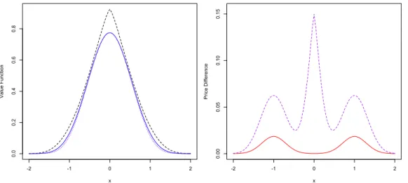
First, we consider a European Butterfly option with three strikes K1 = 1 <

K2 = 0 < K3 = 1, where K1+ 1/(2¯) K2  K3 1/(2¯). Its pay-off is

g(x) = (x K1)+ 2(x K2)++ (x K3)+,

and the corresponding face-lifted function ˆg can be computed explicitly: ˆ g(x) = ¯ 2(x x1) 2₁ [x₁,x+₁)+ (x K1)1[x+₁,K2) +(x K1 2(x K2))1_[K2,x 2) +⇣ ¯ 2(x x + 2)2+ 2K2 (K1+ K3) ⌘ 1_[x 2,x+2) +(2K2 (K1+ K3))1_[x+ 2,+1), where x± 1 = K1± 1/(2¯) and x±2 = K3± 1/(2¯).

In Figure 1, we separately show the effect of the gamma constraint and of the market impact. As observed in Remark 1.9, the price is non-decreasing with respect to the impact parameter and bounded from below by the hedging price obtained in the model without impact nor gamma constraint. On the left and right tails of the curves, we observe the effect of the gamma constraint. It does not operate around x = 0 where the gamma is non-positive. The effect of the market impact operates only in areas of high convexity (around x = 1.5 and x = 1.5) or of high concavity (around x = 0). -2 -1 0 1 2 0.0 0.2 0.4 0.6 0.8 x Va lu e F un ct io n -2 -1 0 1 2 0.00 0.05 0.10 0.15 x Pri ce D iff ere nce

Figure 1: Left: Super-hedging price of the Butterfly option. Dashed line: = 0.5, ¯ = 1.75; solid line: = 0, ¯ = 1.75; dotted line: = 0, ¯ = +1. Right: Difference with the price associated to = 0, ¯ = +1. Dashed line:

= 0.5, ¯ = 1.75; solid line: = 0, ¯ = 1.75 .

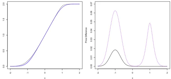
In Figure 2, we perform similar computations but for a call spread option, where

g(x) = (x K1)+ (x K2)+,

with K1 = 1 < K2 = 1 such that K1+ 1/(2¯)  K2. The face-lifted function ˆg

is given by ˆ g(x) = ¯ 2(x x ) 2₁ [x ,x+₎+ (x K₁)1_[x+_,K 2)+ (K2 K1)1[K2,+1) with x±_{= K} 1± 1/(2¯).

-2 -1 0 1 2 0.0 0.5 1.0 1.5 2.0 x Va lu e F un ct io n -2 -1 0 1 2 0.00 0.01 0.02 0.03 0.04 0.05 0.06 0.07 x Pri ce D iff ere nce

Figure 2: Left: Super-hedging price of the Call Spread option. Dashed line: = 0.5, ¯ = 1.75; solid line: = 0, ¯ = 1.75; dotted line: = 0, ¯ = +1. Right: Difference with the price associated to = 0, ¯ = +1. Dashed line:

= 0.5, ¯ = 1.75; solid line: = 0, ¯ = 1.75 .

5 Appendix

The following is very standard, we prove it for completeness.

Lemma 5.1. A upper-semicontinuous (resp. lower-semicontinuous) map is a vis-cosity subsolution (resp. supersolution) of

F_✏[']1[0,T )+ (' gˆ✏K)1{T }= 0

if and only if it is a viscosity subsolution (resp. supersolution) of F✏,K

, ['] = 0(resp.

F_,+✏,K['] = 0).

Proof. The equivalence on [0, T ) is evident, we only consider the parabolic bound-ary {T } ⇥ R. Since F✏,K

,+ F✏ and F,✏,K  F✏, only one implication is not

com-pletely trivial.

a. Let v be a viscosity supersolution of F✏,K

,+['] = 0, and ' 2 C2be a test function

such that

(strict) min